6  Generalized Additive Models

Linear regression is easy to fit and easy to read: each coefficient tells you how the response changes when one predictor moves by one unit, holding the rest fixed. The price for that simplicity is the assumption that every effect is a straight line. Real relationships are rarely so obedient. Wages rise with age and then taper off near retirement; the effect of a neighborhood’s poverty rate on house prices is steep at first and then flattens. We could chase these curves with polynomials, splines, or kernel smoothers (covered in the earlier chapters on spline regression (Chapter 3), kernel smoothing (Chapter 4), and local regression (Chapter 5)), but those tools are usually presented one predictor at a time. Generalized additive models, or GAMs, are the natural way to put several such smooth pieces together in a single, interpretable model.

The idea is to keep the additive structure of linear regression but to replace each straight line with a flexible curve. We learn a separate smooth function for each predictor and then add the pieces up:

\[ E(Y|X_1,X_2,\dots,X_p)= \alpha + f_1(X_1) + f_2(X_2)+ \dots + f_p(X_p) \]

where \(f_j(.),j = 1,\dots, p\) are unspecified smooth (nonparametric) functions.¹

Key idea

A GAM trades the global slope of linear regression for a sum of flexible, predictor-specific curves. It is more expressive than a linear model, yet because the effects still add up you can read off and plot what each predictor does on its own.

This is what the name records: we call the model additive because we keep a separate \(f_j\) for each \(X_j\) and sum them, and generalized because (as we will see) the same idea extends to non-Gaussian responses through a link function. Two properties make the additive form attractive at once. We can fit a complicated curve for each feature, and we can still interpret the model by examining one curve at a time.

Writing the model for a single observation, with an explicit error term, gives the form you will recognize from ordinary regression:

\[ y_i = \alpha + \sum_{j=1}^p f_j (x_{ij}) + \epsilon_i \]

where \(\epsilon\) is usually chosen to follow a Gaussian distribution.

By this point in the book, several of the moving parts should look familiar, and it is worth naming the connections explicitly. If each function \(f_j(.)\) were written as a basis expansion, then we would be back at least squares, GAMs are not a break from regression so much as a flexible generalization of it. A general way to fit each function is a “scatterplot smoother” (for example, a cubic smoothing spline (Chapter 3) or a kernel smoother (Chapter 4)) applied through an algorithm that estimates all \(p\) functions simultaneously. And a transformation of the mean response (a link function), exactly as in Generalized linear models, can be layered on top to handle responses that are not continuous.

Intuition

Think of a GAM as a relay team. Each predictor gets its own smoother to capture its private nonlinear effect, and the link function and additive structure stitch the contributions into one prediction.

6.1 From regression to classification: the link function

The additive idea is not limited to predicting a continuous outcome. Consider a two-group classification problem handled by logistic regression. The quantity we want to model is the conditional probability of the positive class,

\[ \mu(X) = P(Y=1|X) \]

A probability lives between 0 and 1, so we do not model it directly. As in ordinary logistic regression, we model its log-odds, and we let the right-hand side be an additive sum of smooth functions:

\[ \log(\frac{\mu(X)}{1- \mu(X)}) = \alpha + f_1 (X_1) + \dots + f_p(X_p) \]

where each \(f_j\) is an unspecified smooth function. The logit on the left is the link: it maps a probability onto the whole real line so that the additive predictor on the right is free to take any value.

In general, we relate the conditional mean response to the additive function of the predictors through a link function \(g\):

\[ g(\mu(X)) = \alpha + f_1(X_1) + \dots + f_p(X_p) \]

The choice of \(g\) depends on the type of response, and the common cases are exactly those from generalized linear models. The following are the links you will reach for most often:

• \(g(\mu) = \mu\), the identity link, for continuous Gaussian responses.

• \(g(\mu) = logit(\mu)\) or \(g(\mu) = probit(\mu)\), as in the glm case for binary and binomial data (the probit function is the inverse Gaussian cumulative distribution function, \(probit (\mu) = \Phi^{-1}(\mu)\)).

• \(g(\mu) = \log(\mu)\), for Poisson count data.

Note

Choosing the link for a GAM follows the same logic as choosing it for a GLM. Match the link to the distribution of the response, then let the smooth functions handle the shape of each predictor’s effect.

The functions \(f_j\) themselves need not all be nonlinear. Any one of them can be nonlinear, linear, or some other parametric form, and you can mix these freely within a single model. This flexibility lets you build semi-parametric models that model some effects rigidly and others loosely. The following are three useful patterns, each combining parametric and nonparametric pieces:

• \(g(\mu) = X^T \beta + \alpha_k + f(Z)\), a semi-parametric model, where

  • \(X\) is a vector of predictors to be modeled linearly,

  • \(\alpha_k\) is the effect for the \(k\)-th level of a qualitative input \(V\),

  • and the effect of the predictor \(Z\) is modeled nonparametrically.

• \(g(\mu) = f(X) + g_k(Z)\), where \(k\) indexes the levels of a qualitative input \(V\) and thus creates an interaction term with \(Z\), \(g(V,Z) =g_k(Z)\).

• \(g(\mu)= f(X)+g(Z,W)\), where \(g\) is a nonparametric function in two features, \(Z\) and \(W\) (a smooth surface rather than a curve).

When to use this

Reach for a semi-parametric GAM when theory or prior work tells you a particular effect is linear, but you suspect other predictors bend. Modeling the known effect linearly saves degrees of freedom and sharpens interpretation, while the smooth terms absorb the curves you cannot pin down in advance.

6.2 Fitting Additive Models

How do we actually estimate a sum of smooth functions? We start, as so often, by writing down what “a good fit” should mean and then minimizing it. We choose each \(f_j\) to be a smoother and minimize a penalized residual sum of squares:

\[ PRSS(\alpha, f_1,\dots, f_p) = \sum_{i=1}^n (y_i - \alpha- \sum_{j=1}^p f_j(x_{ij}))^2 + \sum_{j=1}^p \lambda_j \int f''_j (t_j)^2 dt_j \]

where the \(\lambda_j \ge 0\) are tuning parameters. The first term rewards fitting the data; the second penalizes wiggliness, since \(\int f''_j(t)^2 dt\) is large when \(f_j\) curves sharply. Each \(\lambda_j\) sets the trade-off for one predictor: large \(\lambda_j\) forces \(f_j\) toward a straight line, while \(\lambda_j = 0\) lets it bend as much as the data demand.²

Intuition

The penalty is a dial for honesty. Turn \(\lambda_j\) up and the curve must justify every wiggle with strong evidence; turn it down and the curve is free to follow noise.

It turns out that the minimizer of this criterion is not some exotic object: it is an additive cubic spline model, with each function \(f_j\) a cubic spline in \(X_j\) that has knots at each of the unique values of \(x_{ij}, i = 1, \dots, n\). The penalty is what keeps such a richly knotted spline from overfitting.

One technical wrinkle is worth flagging before we fit. This solution is not unique because \(\alpha\) is not identifiable without another constraint: you could add a constant to \(\alpha\) and subtract it from one of the \(f_j\) without changing any prediction. To pin it down, we require each smooth to be centered, \(\sum_{i=1}^n f_j(x_{ij})=0 \; \forall j\), which forces \(\hat{\alpha}= ave(y_i)\). The intercept absorbs the overall level, and each curve describes only deviations from it. Uniqueness of the rest of the solution then depends on the design:

• If \(\mathbf{X} = \{x_{ij}\}\) is of full column rank, then the minimizer is unique.

• If this is not the case (that is, \(\mathbf{X'X}\) is singular), then the linear portions of the components \(f_j\) cannot be uniquely determined, but the nonlinear parts can.

Warning

When predictors are collinear, do not over-interpret the straight-line part of any individual curve. The bend of the curve is still trustworthy, but the linear tilt can be shuffled between correlated predictors without changing the fit.

6.2.1 Existence and the projection view of the penalty

Before deriving an algorithm, it helps to know what the penalized criterion is really optimizing. Each penalty \(\int f_j''(t)^2\,dt\) is a quadratic form in the function \(f_j\). If we evaluate \(f_j\) at the \(n\) data points and collect the values into a vector \(\mathbf{f}_j = (f_j(x_{1j}),\dots,f_j(x_{nj}))^\top\), then the cubic smoothing spline penalty can be written exactly as a quadratic form \(\mathbf{f}_j^\top \mathbf{K}_j \mathbf{f}_j\), where \(\mathbf{K}_j\) is a fixed, symmetric, positive semidefinite penalty matrix that depends only on the design points \(\{x_{ij}\}\) (its construction is given in Chapter 3). With \(\mathbf{f} = \sum_j \mathbf{f}_j\) and \(\mathbf{1}\) the vector of ones, the criterion in vector form is

\[ PRSS(\alpha, \mathbf{f}_1,\dots,\mathbf{f}_p) = \Big\| \mathbf{y} - \alpha\mathbf{1} - \sum_{j=1}^p \mathbf{f}_j \Big\|^2 + \sum_{j=1}^p \lambda_j\, \mathbf{f}_j^\top \mathbf{K}_j \mathbf{f}_j . \tag{6.1}\]

This is a strictly convex problem in the centered components (the data-fit term is convex and each penalty is convex, and centering removes the only flat direction, the shared constant), so a minimizer exists and, on the space of centered functions of full-rank predictors, it is unique. Convexity is what guarantees that the iterative scheme below converges to the global optimum rather than to a spurious stationary point.

6.2.2 The Backfitting Algorithm for Additive Models

There is no closed-form formula that solves all \(p\) smoothers at once, so we fit the model with a simple iterative scheme called backfitting. The intuition is one of polite turn-taking: to update one function, hold the others fixed, strip their contributions out of the response, and smooth what remains. Concretely, let \(S_j\) be the cubic smoothing spline for the \(j\)-th function. We apply it to the partial residuals \(\{y_i - \hat{\alpha} - \sum_{k \neq j}\hat{f}(x_{ik}) \}^n_1\), viewed as a function of \(x_{ij}\), to obtain the new estimate \(\hat{f}_j\). We repeat this for each predictor, always using the current estimates of the other functions when forming the residuals, and we keep cycling until the estimates \(\hat{f}_j\) stabilize.

Intuition

Backfitting is “explain what’s left over.” Each curve takes a turn explaining the part of the response that the other curves have not yet accounted for, and the curves keep refining one another until nothing changes.

Written out as a procedure, the algorithm has two steps. Step 1 initializes the intercept to the mean and every curve to zero:

\[ \hat{\alpha} = \frac{1}{N}\sum_{1}^N y_i, \hat{f}_j \equiv 0, \forall i, j \]

Step 2 cycles through the predictors \(j = 1,2, \dots, p, \dots, 1, 2, \dots, p, \dots\), smoothing the partial residuals and then re-centering each updated curve:

\[ \hat{f}_j \leftarrow S_j [\{ y_i - \hat{\alpha}- \sum_{k \neq j} \hat{f}_k (x_{ik})\}^N_1] \]

\[ \hat{f}_j \leftarrow \hat{f}_j - \frac{1}{N} \sum_{i=1}^N \hat{f}_j (x_{ij}) \]

The cycle continues until the functions \(\hat{f}_j\) change by less than a prespecified threshold. The re-centering line is just the identifiability constraint from above, enforced at every update so that each curve keeps describing deviations from \(\hat\alpha\).

6.2.2.1 Why backfitting is the right update

The backfitting step is not an ad hoc heuristic: it is exactly the coordinate-wise minimizer of Equation 6.1. Fix all components except the \(j\)-th and treat \(\mathbf{f}_j\) as the only free variable. Collecting the terms that involve \(\mathbf{f}_j\), the criterion is

\[ \Big\| \big(\mathbf{y} - \alpha\mathbf{1} - \textstyle\sum_{k\neq j}\mathbf{f}_k\big) - \mathbf{f}_j \Big\|^2 + \lambda_j\, \mathbf{f}_j^\top \mathbf{K}_j \mathbf{f}_j . \]

Writing \(\mathbf{r}_j = \mathbf{y} - \alpha\mathbf{1} - \sum_{k\neq j}\mathbf{f}_k\) for the partial residual, this is precisely the objective of a single smoothing spline applied to \(\mathbf{r}_j\). Differentiating with respect to \(\mathbf{f}_j\) and setting the gradient to zero,

\[ -2(\mathbf{r}_j - \mathbf{f}_j) + 2\lambda_j \mathbf{K}_j \mathbf{f}_j = 0 \;\;\Longrightarrow\;\; (\mathbf{I} + \lambda_j \mathbf{K}_j)\,\mathbf{f}_j = \mathbf{r}_j \;\;\Longrightarrow\;\; \hat{\mathbf{f}}_j = (\mathbf{I} + \lambda_j \mathbf{K}_j)^{-1}\mathbf{r}_j = \mathbf{S}_j\,\mathbf{r}_j . \tag{6.2}\]

The matrix \(\mathbf{S}_j = (\mathbf{I} + \lambda_j \mathbf{K}_j)^{-1}\) is the smoother matrix of the cubic smoothing spline, so applying \(S_j\) to the partial residuals is the same as solving the one-dimensional penalized problem in closed form. Backfitting therefore cycles through these blocks, and each pass is one sweep of block Gauss-Seidel (equivalently block coordinate descent) on a convex quadratic. The stacked stationarity conditions for all \(p\) blocks form the linear system

\[ \begin{pmatrix} \mathbf{I} & \mathbf{S}_1 & \cdots & \mathbf{S}_1 \\ \mathbf{S}_2 & \mathbf{I} & \cdots & \mathbf{S}_2 \\ \vdots & & \ddots & \vdots \\ \mathbf{S}_p & \mathbf{S}_p & \cdots & \mathbf{I} \end{pmatrix} \begin{pmatrix}\mathbf{f}_1\\ \mathbf{f}_2\\ \vdots\\ \mathbf{f}_p\end{pmatrix} = \begin{pmatrix}\mathbf{S}_1\mathbf{y}\\ \mathbf{S}_2\mathbf{y}\\ \vdots\\ \mathbf{S}_p\mathbf{y}\end{pmatrix}, \tag{6.3}\]

and backfitting is the Gauss-Seidel iteration for this system. Convergence: if every smoother \(\mathbf{S}_j\) is a symmetric operator with eigenvalues in \([0,1]\) (true for cubic smoothing splines), the backfitting map is a contraction on the centered space and the iterates converge to the unique solution of Equation 6.3; when two predictors are exactly collinear the system Equation 6.3 is singular and only the sum \(\mathbf{f}_1+\mathbf{f}_2\) is determined, which is the concrete form of the non-identifiability flagged above. This is also why backfitting can converge slowly when predictors are strongly correlated: the off-diagonal blocks are large, so the Gauss-Seidel iteration mixes the components slowly, exactly as Gauss-Seidel slows for ill-conditioned linear systems.

Note

The update Equation 6.2 is the additive-model analogue of the normal equations. In ordinary least squares we invert \(\mathbf{X}^\top\mathbf{X}\) once; here each block has its own simple inverse \((\mathbf{I}+\lambda_j\mathbf{K}_j)^{-1}\), and backfitting stitches the blocks together iteratively because no single closed form solves all of them jointly at reasonable cost.

Two features of backfitting make it a workhorse rather than a one-off recipe. First, it is modular: any smoother can take the place of \(S_j\), so you can mix and match the right tool for each predictor. The available choices include the following.

• Other univariate regression smoothers, for example local polynomial regression (Chapter 5) and kernel smoothing (Chapter 4).

• Linear regression operators yielding polynomial fits, piecewise constant fits, parametric spline fits, or Fourier series fits.

• Smoothers for second or higher-order interactions, or periodic smoothers for seasonal effects.

Second, backfitting gives us an honest accounting of model complexity. If we evaluate the smoother at the training points, it can be represented by the \(n \times n\) smoother matrix \(\mathbf{S}_j\), and the effective degrees of freedom for the \(j\)-th term can be estimated from \(trace(\mathbf{S}_j) -1\). This is the number we report when we say a term “uses about 4 degrees of freedom,” and it lets us compare a smooth term against, say, a quartic polynomial on a common scale.

6.2.3 Penalized regression splines and choosing the smoothing parameter

The smoothing-spline view above puts a knot at every distinct value of each predictor, which makes the smoother matrices \(n\times n\) and the fit expensive for large \(n\). The mgcv package used in Example 2 takes the more scalable penalized regression spline route, and it is worth deriving because it also makes the automatic smoothness selection (the “we never told mgcv how many knots to use” payoff) concrete.

Represent each smooth in a fixed, moderate basis of size \(K_j \ll n\),

\[ f_j(x) = \sum_{m=1}^{K_j} \beta_{jm}\,b_{jm}(x), \]

where \(b_{jm}\) are spline basis functions (for example thin-plate or cubic-regression bases). Stacking the evaluations gives a model matrix \(\mathbf{X}\) with one block of columns per smooth, and the wiggliness penalty becomes quadratic in the coefficients, \(\int f_j''(t)^2\,dt = \boldsymbol\beta_j^\top \mathbf{S}_j \boldsymbol\beta_j\) for a fixed penalty matrix \(\mathbf{S}_j\). The Gaussian objective is then a single penalized least squares problem in \(\boldsymbol\beta\),

\[ \| \mathbf{y} - \mathbf{X}\boldsymbol\beta \|^2 + \sum_j \lambda_j\,\boldsymbol\beta^\top \mathbf{S}_j \boldsymbol\beta = \| \mathbf{y} - \mathbf{X}\boldsymbol\beta \|^2 + \boldsymbol\beta^\top \mathbf{S}_\lambda \boldsymbol\beta, \qquad \mathbf{S}_\lambda = \sum_j \lambda_j \mathbf{S}_j , \]

which, unlike the backfitting system, has a genuine ridge-type closed form. Setting the gradient to zero,

\[ \hat{\boldsymbol\beta} = (\mathbf{X}^\top\mathbf{X} + \mathbf{S}_\lambda)^{-1}\mathbf{X}^\top\mathbf{y}, \qquad \hat{\mathbf{y}} = \mathbf{A}_\lambda \mathbf{y}, \quad \mathbf{A}_\lambda = \mathbf{X}(\mathbf{X}^\top\mathbf{X} + \mathbf{S}_\lambda)^{-1}\mathbf{X}^\top . \tag{6.4}\]

The matrix \(\mathbf{A}_\lambda\) is the GAM analogue of the hat matrix, and its trace defines the effective degrees of freedom of the whole model, \(\mathrm{edf} = \mathrm{tr}(\mathbf{A}_\lambda)\). As \(\lambda_j\to 0\) the penalty vanishes and \(\mathrm{edf}\to \mathrm{rank}(\mathbf{X})\); as \(\lambda_j\to\infty\) the smooth is forced into the null space of \(\mathbf{S}_j\) (a straight line for the second-derivative penalty), so \(\mathrm{edf}\) shrinks toward the dimension of that null space. This is the precise sense in which the penalty, not the knot count, controls flexibility: with \(K_j\) large enough to be flexible, \(\lambda_j\) alone decides how much of that flexibility is used.

The smoothing parameters are chosen by minimizing a prediction-error criterion rather than by hand. Generalized cross-validation (GCV) uses a rotation-invariant approximation to leave-one-out error,

\[ \mathrm{GCV}(\lambda) = \frac{n\,\|\mathbf{y} - \mathbf{A}_\lambda\mathbf{y}\|^2}{\big(n - \mathrm{tr}(\mathbf{A}_\lambda)\big)^2}, \tag{6.5}\]

obtained from ordinary cross-validation by replacing each leverage \(A_{ii}\) with the average leverage \(\mathrm{tr}(\mathbf{A}_\lambda)/n\). The denominator penalizes models that spend many effective degrees of freedom, so GCV trades fit against complexity automatically. Modern mgcv defaults instead to maximizing a (restricted) marginal likelihood, which treats \(\boldsymbol\beta\sim N(\mathbf{0}, \mathbf{S}_\lambda^{-}/\,)\) as a Gaussian prior and is generally more resistant to the occasional severe undersmoothing that GCV can produce; both deliver the same automatic-smoothness behavior, and both are far cheaper than searching a grid of knot positions by hand.

When to use this

Prefer the mgcv penalized-regression-spline machinery for anything beyond small data: it scales as \(O(nK^2)\) rather than \(O(n^3)\), selects all \(\lambda_j\) jointly by GCV or REML, and reports an honest per-term \(\mathrm{edf}\). Reserve the classic per-knot smoothing spline plus backfitting (the gam package) for pedagogy or when you want to plug in a nonstandard smoother such as lo.

We can confirm the penalized-least-squares solution Equation 6.4 and the effective-degrees-of-freedom identity \(\mathrm{edf}=\mathrm{tr}(\mathbf{A}_\lambda)\) on a tiny example with base R. As \(\lambda\) grows the fit stiffens and the trace of the influence matrix falls toward the dimension of the penalty null space.

set.seed(1)
n <- 60
x <- sort(runif(n))
y <- sin(2 * pi * x) + rnorm(n, sd = 0.3)

# cubic B-spline basis and a second-difference penalty (P-spline)
X <- splines::bs(x, df = 12, intercept = TRUE)
D <- diff(diag(ncol(X)), differences = 2)   # second-difference operator
S <- crossprod(D)                            # penalty matrix S = D'D

edf <- function(lambda) {
  A <- X %*% solve(crossprod(X) + lambda * S, t(X))  # influence (hat) matrix
  sum(diag(A))
}

# beta-hat from eq-gam.qmd-pls-solution equals the closed-form ridge solution
lambda <- 1
beta_hat <- solve(crossprod(X) + lambda * S, crossprod(X, y))
fit_direct <- as.vector(X %*% beta_hat)
fit_hat    <- as.vector(X %*% solve(crossprod(X) + lambda * S, t(X)) %*% y)
max(abs(fit_direct - fit_hat))                # ~0: same fitted values
#> [1] 8.881784e-16

sapply(c(0, 0.01, 1, 100, 1e6), edf)          # edf decreases as lambda grows
#> [1] 12.000000 11.014938  6.156837  2.775369  2.000147

The first number is essentially zero (the two ways of writing the fit agree), and the effective degrees of freedom decrease monotonically from the full basis dimension toward 2, the dimension of the second-difference penalty null space (the space of straight lines), exactly as the theory predicts.

6.3 Fitting Generalized Additive Models

So far the response has been Gaussian and the loss has been squared error. When the response is binary, count, or otherwise non-Gaussian, we swap squared error for the negative log-likelihood, exactly as generalized linear models do, and we maximize a penalized log-likelihood instead. The fitting strategy combines the backfitting procedure with a likelihood maximizer: the weighted linear regression component that a GLM would solve is replaced by a weighted backfitting algorithm, Hastie, Friedman, and Tibshirani (2001) (section 9.2).

Key idea

A GAM is to a GLM what an additive model is to linear regression. Keep the GLM machinery (link function, iteratively reweighted fitting) and replace the linear predictor with a sum of smooths.

6.3.1 Local Scoring Algorithm

The concrete algorithm for the logistic case is called local scoring. It wraps backfitting inside the same iteratively reweighted least squares loop you saw for logistic regression: at each pass we form a working response and weights from the current fit, then run a weighted additive fit on them.

Step 1 initializes the intercept to the log-odds of the overall positive rate and sets every curve to zero. Compute \(\hat{\alpha} = \log [\frac{\bar{y}}{1- \bar{y}}]\), where \(\bar{y} = ave(y_i)\) is the sample proportion of ones, and set \(\hat{f}_j\equiv 0 \; \forall j\).

Step 2 defines the current additive predictor and the implied fitted probabilities, \(\hat{\eta}_i = \hat{\alpha} + \sum_j \hat{f}_j(x_{ij})\) and \(\hat{p}_i = \frac{1}{1 + \exp(-\hat{\eta}_i)}\), and then iterates the following three substeps:

1. Construct the working target variable: \(z_i = \hat{\eta}_i + \frac{y_i - \hat{p}_i}{\hat{p}_i(1-\hat{p}_i)}\).
2. Construct weights \(w_i = \hat{p}_i (1-\hat{p}_i)\).
3. Fit an additive model to the targets \(z_i\) with weights \(w_i\), using a weighted backfitting algorithm. This gives new estimates \(\hat{\alpha}, \hat{f}_j, \forall j\).

Step 3 continues step 2 until the change in the functions falls below a pre-specified threshold.

Note

The working target \(z_i\) is a local linear approximation to the link applied to the response, and the weights \(w_i\) are the variance of a Bernoulli draw with probability \(\hat p_i\). Observations whose probabilities are near 0 or 1 carry little weight, which is the same reweighting that drives standard logistic regression.

6.3.1.1 Deriving the working response and weights

The working response and weights are not memorized formulas; they fall out of a Newton (Fisher scoring) step on the penalized log-likelihood, exactly as in a GLM. Write \(\eta_i = \alpha + \sum_j f_j(x_{ij})\) for the additive predictor and let the response have a one-parameter exponential-family distribution with mean \(\mu_i\), link \(g(\mu_i)=\eta_i\), and variance function \(V(\mu_i)\). The penalized log-likelihood to be maximized is

\[ \ell_p = \sum_{i=1}^n \ell(y_i; \mu_i) - \tfrac12 \sum_j \lambda_j \int f_j''(t)^2\,dt . \]

Consider the score with respect to \(\eta_i\). For an exponential family the per-observation score has the standard form

\[ \frac{\partial \ell_i}{\partial \eta_i} = \frac{y_i - \mu_i}{V(\mu_i)}\,\frac{\partial \mu_i}{\partial \eta_i}, \qquad -\,\mathbb{E}\!\left[\frac{\partial^2 \ell_i}{\partial \eta_i^2}\right] = \frac{1}{V(\mu_i)}\left(\frac{\partial \mu_i}{\partial \eta_i}\right)^2 =: w_i , \]

where \(w_i\) is the Fisher information for \(\eta_i\), i.e. the IRLS weight. A single Fisher-scoring update solves a quadratic approximation to \(\ell_p\) around the current \(\hat\eta_i\). Completing the square, that quadratic is, up to constants, a weighted penalized least squares problem in the new predictor \(\eta\),

\[ \sum_{i=1}^n w_i (z_i - \eta_i)^2 + \sum_j \lambda_j \int f_j''(t)^2\,dt, \qquad z_i = \hat\eta_i + (y_i - \hat\mu_i)\,\frac{\partial \eta_i}{\partial \mu_i} = \hat\eta_i + (y_i - \hat\mu_i)\,g'(\hat\mu_i), \tag{6.6}\]

which is the adjusted dependent variable. Specializing to logistic regression makes the displayed formulas appear: with \(g=\mathrm{logit}\) we have \(\mu_i = p_i\), \(g'(\mu_i) = 1/[p_i(1-p_i)]\), and \(V(\mu_i)=p_i(1-p_i)\), so

\[ w_i = \frac{(\partial \mu_i/\partial\eta_i)^2}{V(\mu_i)} = \frac{[p_i(1-p_i)]^2}{p_i(1-p_i)} = p_i(1-p_i), \qquad z_i = \hat\eta_i + \frac{y_i - \hat p_i}{\hat p_i(1-\hat p_i)} , \]

exactly the weights and working target in the algorithm above. The inner “fit an additive model to \(z_i\) with weights \(w_i\)” step is therefore the weighted version of the backfitting normal equations Equation 6.2, with the unweighted smoother \(\mathbf{S}_j\) replaced by its weighted form \(\mathbf{S}_j^{(w)} = (\mathbf{W} + \lambda_j \mathbf{K}_j)^{-1}\mathbf{W}\). Local scoring is thus a doubly nested loop: an outer Fisher-scoring (IRLS) loop that rebuilds \((z_i, w_i)\), and an inner backfitting loop that solves the weighted additive least squares problem. Because each outer step is a Newton step on a concave penalized log-likelihood (concave for canonical links), it inherits the local quadratic convergence of Newton’s method once the iterates are near the optimum.

6.4 Theoretical properties and practical guidance

6.4.1 Why additivity beats the curse of dimensionality

The deepest reason GAMs are useful is a rate result. A fully nonparametric estimator of a \(p\)-dimensional regression surface \(E(Y\mid X)=m(X)\) with two bounded derivatives converges at the rate \(n^{-4/(4+p)}\) in mean squared error: the exponent collapses toward zero as \(p\) grows, which is the curse of dimensionality. Stone (1985, 1986) showed that if the regression function is genuinely additive, \(m(X)=\alpha+\sum_j f_j(X_j)\) with each \(f_j\) twice differentiable, then each component, and hence the whole fit, can be estimated at the one-dimensional optimal rate

\[ \mathbb{E}\big[(\hat f_j(x) - f_j(x))^2\big] = O\!\big(n^{-4/5}\big), \]

independent of \(p\). The additive constraint converts a \(p\)-dimensional smoothing problem into \(p\) one-dimensional ones, and that is precisely what restores a usable convergence rate. The price is bias: if the truth contains interactions, no additive model can represent them, so \(\hat m\) is asymptotically biased no matter how large \(n\) is. This is the bias-variance bargain of the method, lower variance and a fast rate in exchange for an approximation (modeling) bias whenever additivity fails.

6.4.2 Standard errors, inference, and the “p-value for a curve”

Because each fit at the data points is linear in \(\mathbf{y}\), \(\hat f_j = \mathbf{S}_j^{\text{(full)}}\mathbf{y}\) for an appropriate row block, pointwise variance bands follow from \(\mathrm{Var}(\hat f_j) = \sigma^2 \mathbf{S}_j^{\text{(full)}}\mathbf{S}_j^{\text{(full)\top}}\), which is what the se = TRUE bands in the figures display. The “Anova for Nonparametric Effects” table in the gam summary tests whether the nonlinear part of a term is needed by comparing the term’s \(\mathrm{edf}\) against its linear projection on an approximate \(\chi^2\) (or \(F\)) scale; this is the formal version of the visual judgment that year is straight while age bends. In mgcv, the per-smooth p-value is computed from a Wald-type statistic on \(\hat{\boldsymbol\beta}_j\) using a rank-truncated pseudo-inverse of its covariance, and these p-values are approximate because they condition on the selected \(\lambda_j\) (they do not account for the smoothing-parameter estimation, so treat borderline values cautiously).

6.4.3 Failure modes

Three failure modes recur in practice.

• Concurvity, the nonparametric analogue of collinearity: if one smooth term can be well approximated by a function of the others (for example \(X_2 \approx h(X_1)\)), the components trade variance back and forth, standard errors are understated, and the individual curves become unstable even though predictions stay reasonable. mgcv::concurvity() quantifies it; the cure is the same as for collinearity, drop or combine the redundant predictors.

• Boundary and sparse-region instability: smooths are poorly determined where data are thin, producing the wide bands and wild swings seen at the edges of age. The empty education cell in Example 1 is the discrete version of this, an estimated logit driven to \(\pm\infty\), which is exactly why the chapter drops the lowest education level before refitting.

• Missed interactions: additivity is an assumption, not a conclusion. If age and year truly interact, the additive fit averages over the interaction and can be badly biased; the remedy is an explicit tensor-product or bivariate smooth (the lo(year, age) surface and mgcv::te() / ti() terms) for the suspected pair.

6.4.4 Hyperparameters and diagnostics

The only real tuning knobs are the per-term smoothing parameters \(\lambda_j\) (equivalently the target \(\mathrm{edf}\) or df). With mgcv these are selected automatically by GCV or REML, and the practitioner sets only the basis dimension k, which is an upper bound on flexibility rather than the flexibility itself: choose k generously and let the penalty shrink it, then verify with mgcv::gam.check(), whose k-index and residual-vs-fitted diagnostics flag a basis that is too small. With the classic gam package the df argument fixes the \(\mathrm{edf}\) directly and is typically chosen by comparing nested models on an F-test, as Example 1 does. For inference and prediction, report each term’s \(\mathrm{edf}\) (a smooth using near 1 df is effectively linear, a strong signal to simplify the term), inspect partial-residual plots for systematic structure the smooth missed, and remember the computational scaling: \(O(n^3)\) per smoother for full smoothing splines versus \(O(nK^2)\) for penalized regression splines, which is why mgcv is the default for anything but small \(n\).

6.5 Summary

GAMs occupy a useful middle ground: more flexible than linear models, more interpretable than a black box. Table 6.1 weighs what you gain against what you give up.

Table 6.1: Advantages and limitations of generalized additive models.

Pros	Cons
we can fit a nonlinear \(f_j\) to each \(X_j\) and automatically model nonlinear relationships (which we can’t do under standard linear regression)	Model is restricted to be additive. Technically, we can include interactions, but we have to make them manually, and we can only do so with low-dimensional interaction terms as additive functions |
The nonlinear fits can make more accurate predictions | Difficult to fit in high dimensions (because all variables have to be fit) |
Since the model is additive, we can examine the effect of each \(X_j\) on \(Y\) individually while holding all of the other variables fixed (interprebility)
The smoothness of the function \(f_j\) for the variable \(X_j\) can be summarized by df

When to use this

GAMs shine when you have a moderate number of predictors, you expect smooth nonlinear effects, and you still need to explain each effect to a stakeholder. If interactions dominate or the predictor count is very large, a tree-based method such as random forests (Chapter 13) or gradient boosting (Chapter 11), which learns interactions automatically, may serve you better.

The chief limitation, additivity, can be relaxed at a cost. An extension of GAM that includes random effects is called the Generalized Additive Mixed Model (GAMM), useful when observations are grouped or correlated (you can refer to this book³).

6.6 Application

Two worked examples follow. The first uses the gam package to fit and compare several GAMs on a wage dataset, including a logistic GAM for a binary outcome. The second uses mgcv to fit a single smooth on housing data and to evaluate it on a held-out test set. As you read the code, watch how each s(...) term corresponds to one of the smooth functions \(f_j\) from the theory above, and how plotting the model shows those curves directly.

Warning

Both the gam and mgcv packages export a function called gam() and a smoother called s(). Whichever package is loaded last wins. In the examples below the order is intentional; if you mix the two in your own session, call them explicitly (for example gam::gam and gam::s, or mgcv::gam and mgcv::s) to avoid silently using the wrong one.

6.6.1 Example 1

[James et al. (2013), 7.8]

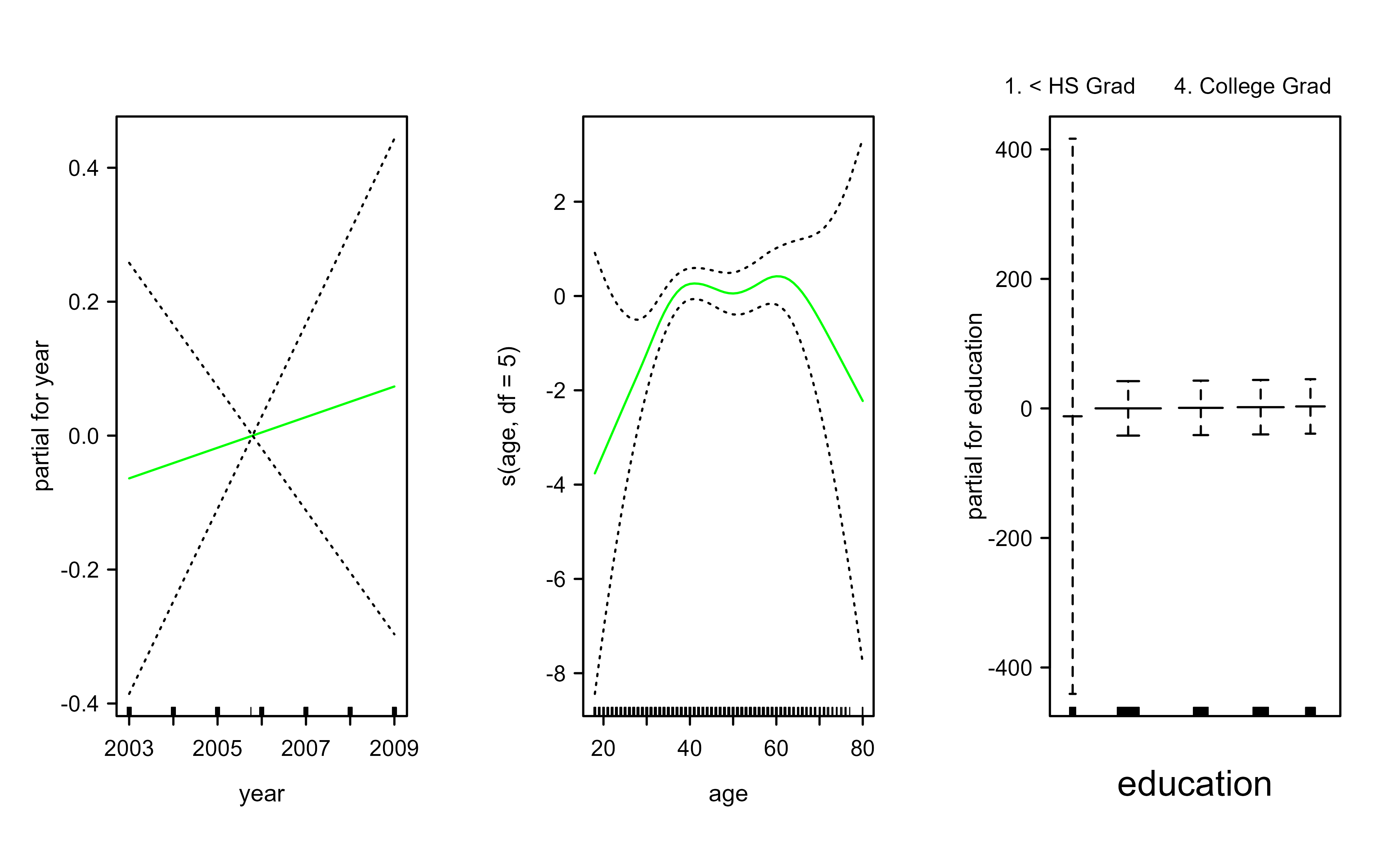
We begin by fitting the model two ways. First we use lm with natural splines, then we refit with smoothing splines through the gam package. Figure 6.1 plots the three smooth-spline components, and Figure 6.2 plots the natural-spline fit for comparison; both show a gently rising year effect and a hump-shaped age effect.

library(ISLR2)
attach(Wage)
library (splines)

# we want to predict for a grid of values for age
agelims <- range (age)
age.grid <- seq (from = agelims[1], to = agelims [2])

# since gam is just linear regresion with transformation of inputs, we can also use lm in R
gam1 <- lm(wage ~ ns(year, 4) + ns(age, 5) + education, data = Wage) # using natural splines

library(gam)
# gam and mgcv both define gam() and s(); this example uses the gam package, so
# make sure it wins the search path even if mgcv was attached elsewhere.
if ("package:mgcv" %in% search()) detach("package:mgcv")
gam.m3 <-
    gam(wage ~ s(year, 4) + s(age, 5) + education, data = Wage) # using smoothing splines

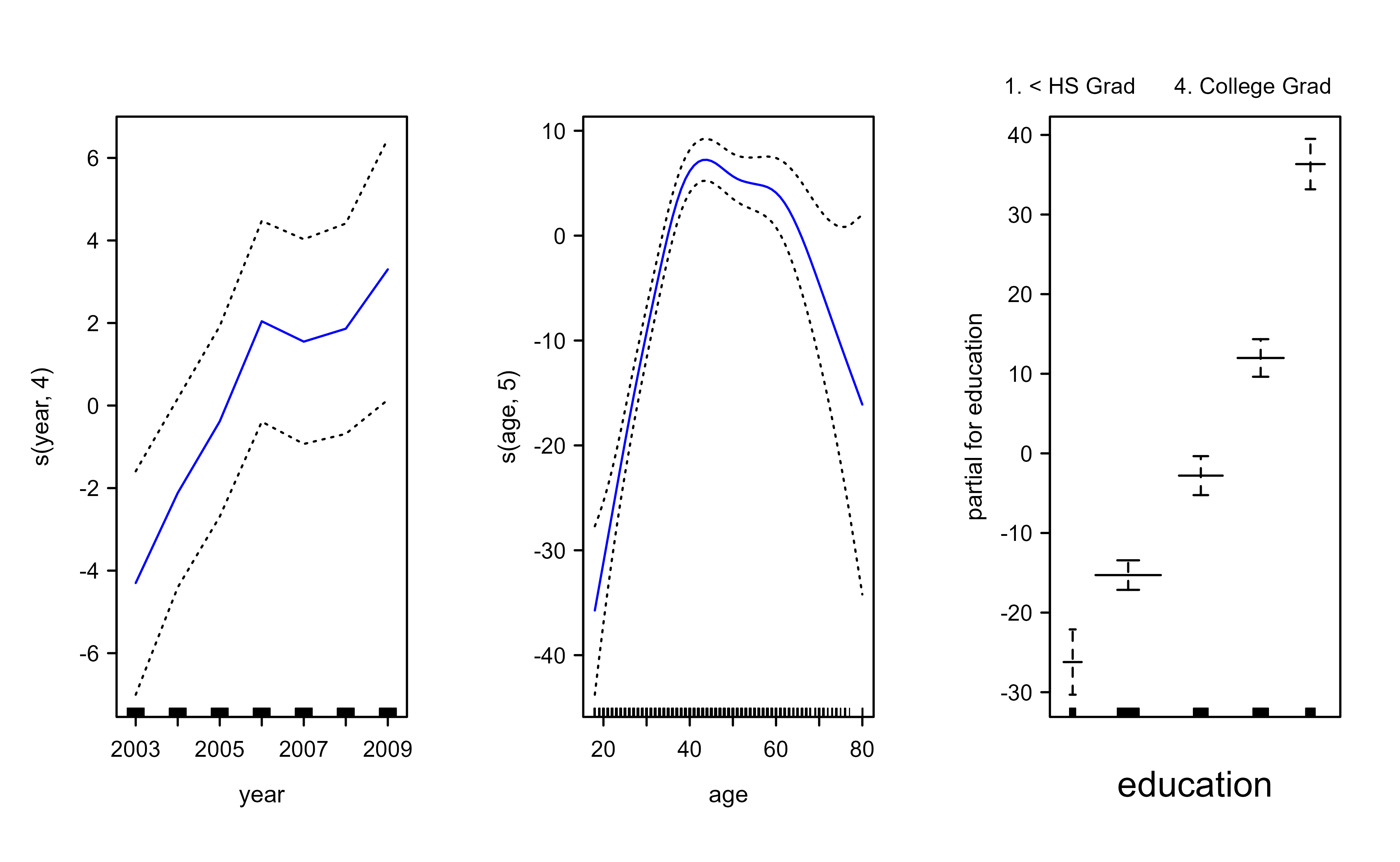
par(mfrow = c(1, 3))
plot(gam.m3, se = T, col = "blue")

Figure 6.1: Smoothing-spline components of the GAM for wage. Each panel shows the estimated smooth effect of year, age, and education, with pointwise standard-error bands.

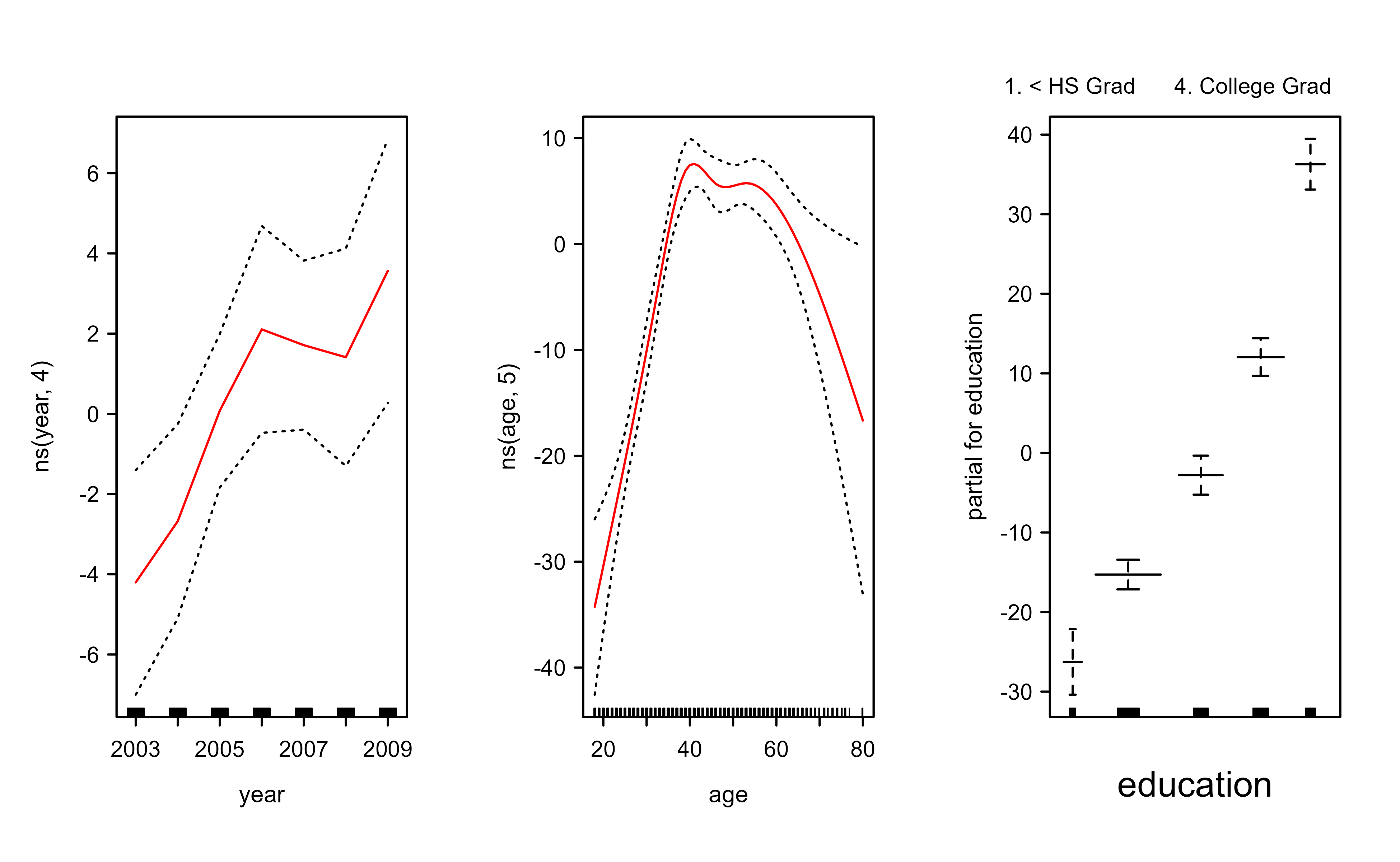
par(mfrow = c(1, 3))
plot.Gam(gam1, se = T, col = "red") # the function of year is rather linear

Figure 6.2: Natural-spline components of the wage model fitted with lm. The estimated effect of year is close to linear, while the effect of age is clearly curved.

The natural-spline fit in Figure 6.2 already hints that the year effect is close to a straight line. We can test this formally by comparing three nested models with an F-test.

if ("package:mgcv" %in% search()) detach("package:mgcv")
gam.m1 <- gam(wage ~ s(age, 5) + education, data = Wage)
gam.m2 <- gam(wage ~ year + s(age, 5) + education, data = Wage)
anova(gam.m1, gam.m2, gam.m3, test = "F") # model 2 is the best one
#> Analysis of Deviance Table
#> 
#> Model 1: wage ~ s(age, 5) + education
#> Model 2: wage ~ year + s(age, 5) + education
#> Model 3: wage ~ s(year, 4) + s(age, 5) + education
#>   Resid. Df Resid. Dev Df Deviance       F    Pr(>F)    
#> 1      2990    3711731                                  
#> 2      2989    3693842  1  17889.2 14.4771 0.0001447 ***
#> 3      2986    3689770  3   4071.1  1.0982 0.3485661    
#> ---
#> Signif. codes:  0 '***' 0.001 '**' 0.01 '*' 0.05 '.' 0.1 ' ' 1

summary(gam.m3)
#> 
#> Call: gam(formula = wage ~ s(year, 4) + s(age, 5) + education, data = Wage)
#> Deviance Residuals:
#>     Min      1Q  Median      3Q     Max 
#> -119.43  -19.70   -3.33   14.17  213.48 
#> 
#> (Dispersion Parameter for gaussian family taken to be 1235.69)
#> 
#>     Null Deviance: 5222086 on 2999 degrees of freedom
#> Residual Deviance: 3689770 on 2986 degrees of freedom
#> AIC: 29887.75 
#> 
#> Number of Local Scoring Iterations: NA 
#> 
#> Anova for Parametric Effects
#>              Df  Sum Sq Mean Sq F value    Pr(>F)    
#> s(year, 4)    1   27162   27162  21.981 2.877e-06 ***
#> s(age, 5)     1  195338  195338 158.081 < 2.2e-16 ***
#> education     4 1069726  267432 216.423 < 2.2e-16 ***
#> Residuals  2986 3689770    1236                      
#> ---
#> Signif. codes:  0 '***' 0.001 '**' 0.01 '*' 0.05 '.' 0.1 ' ' 1
#> 
#> Anova for Nonparametric Effects
#>             Npar Df Npar F  Pr(F)    
#> (Intercept)                          
#> s(year, 4)        3  1.086 0.3537    
#> s(age, 5)         4 32.380 <2e-16 ***
#> education                            
#> ---
#> Signif. codes:  0 '***' 0.001 '**' 0.01 '*' 0.05 '.' 0.1 ' ' 1

preds <- predict(gam.m2, newdata = Wage)

The anova comparison and the summary output tell the same story in two ways. The F-test prefers the model with a linear year term and a smooth age term (model 2), and the “Anova for Nonparametric Effects” block in the summary confirms it: the nonlinear part of age is strongly significant, while the nonlinear part of year is not. In words, age bends the wage curve but year is essentially a straight-line effect, which is exactly what the plotted curves show.

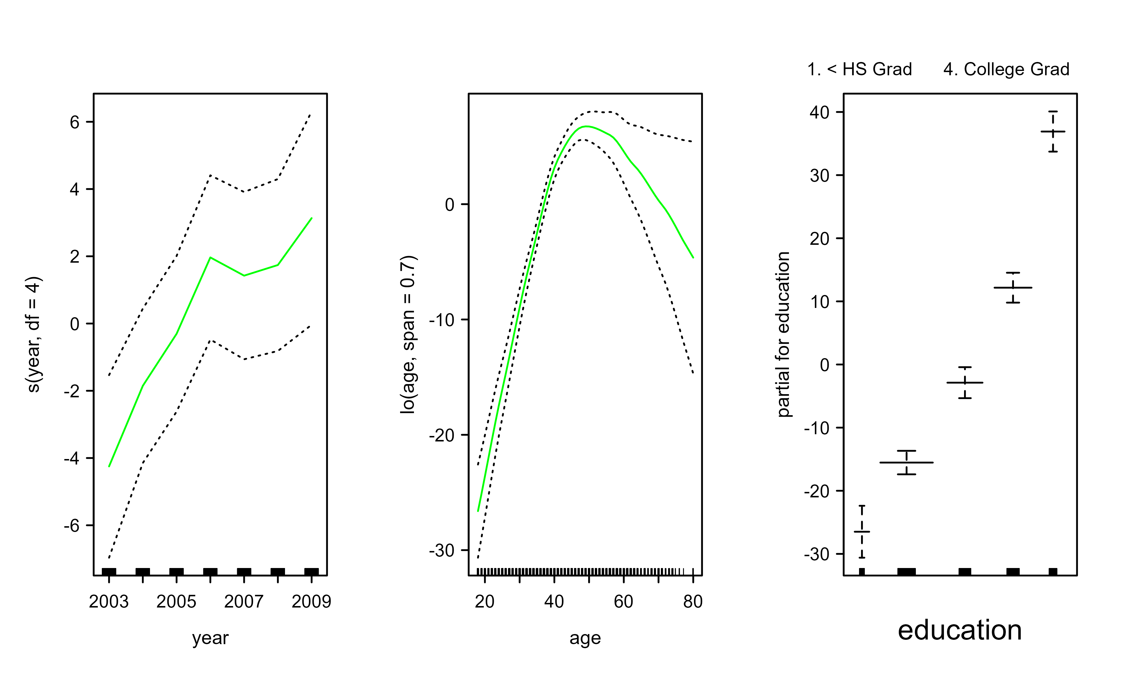
We can also build a GAM from local-regression smoothers. Figure 6.3 replaces the smoothing spline on age with a lo local-regression term.

if ("package:mgcv" %in% search()) detach("package:mgcv")
gam.lo <- gam(wage ~ s(year, df = 4) + lo(age, span = 0.7) + education, data = Wage)
par(mfrow = c(1, 3))
plot.Gam(gam.lo , se = T, col = "green")

Figure 6.3: GAM for wage using a local-regression smoother for age. The year term is a degree-four spline and the age term is a loess fit with span 0.7.

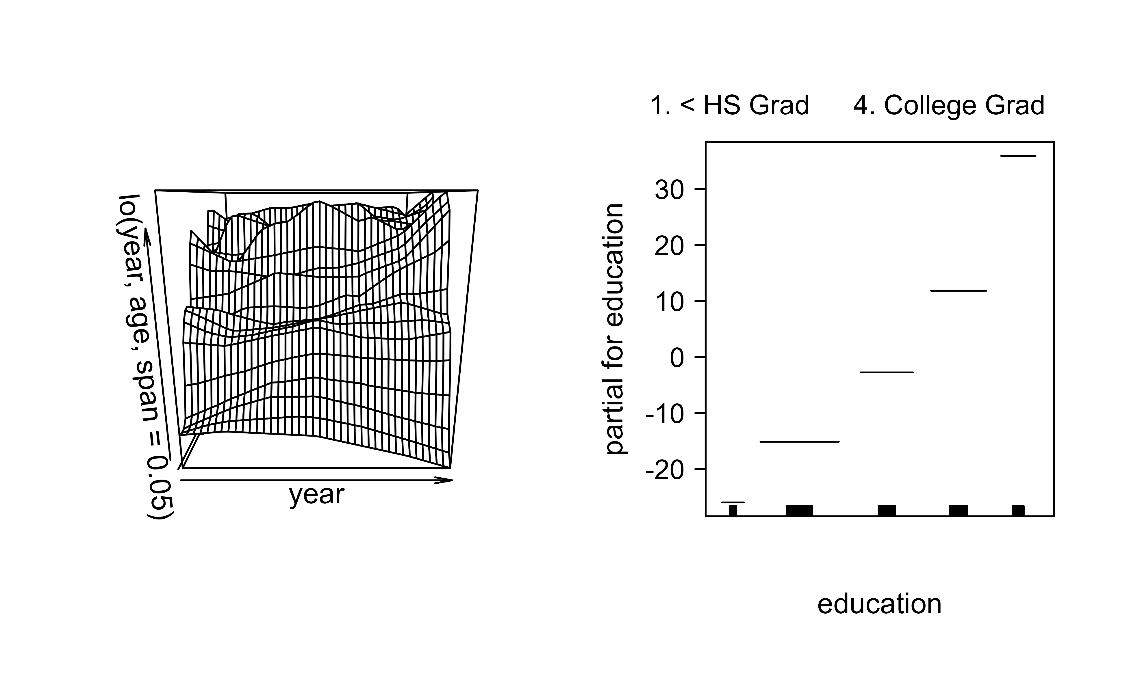
Local regression can also model a two-dimensional smooth surface in year and age jointly, as shown in Figure 6.4.

if ("package:mgcv" %in% search()) detach("package:mgcv")
# using local regression as building blocks for GAM
gam.lo.i <-
    gam(wage ~ lo(year, age, span = .05) + education, data = Wage)

library(akima)
par(mfrow = c(1, 2))
plot(gam.lo.i)

Figure 6.4: Two-dimensional local-regression surface for the joint effect of year and age on wage, fitted as a single bivariate loess term.

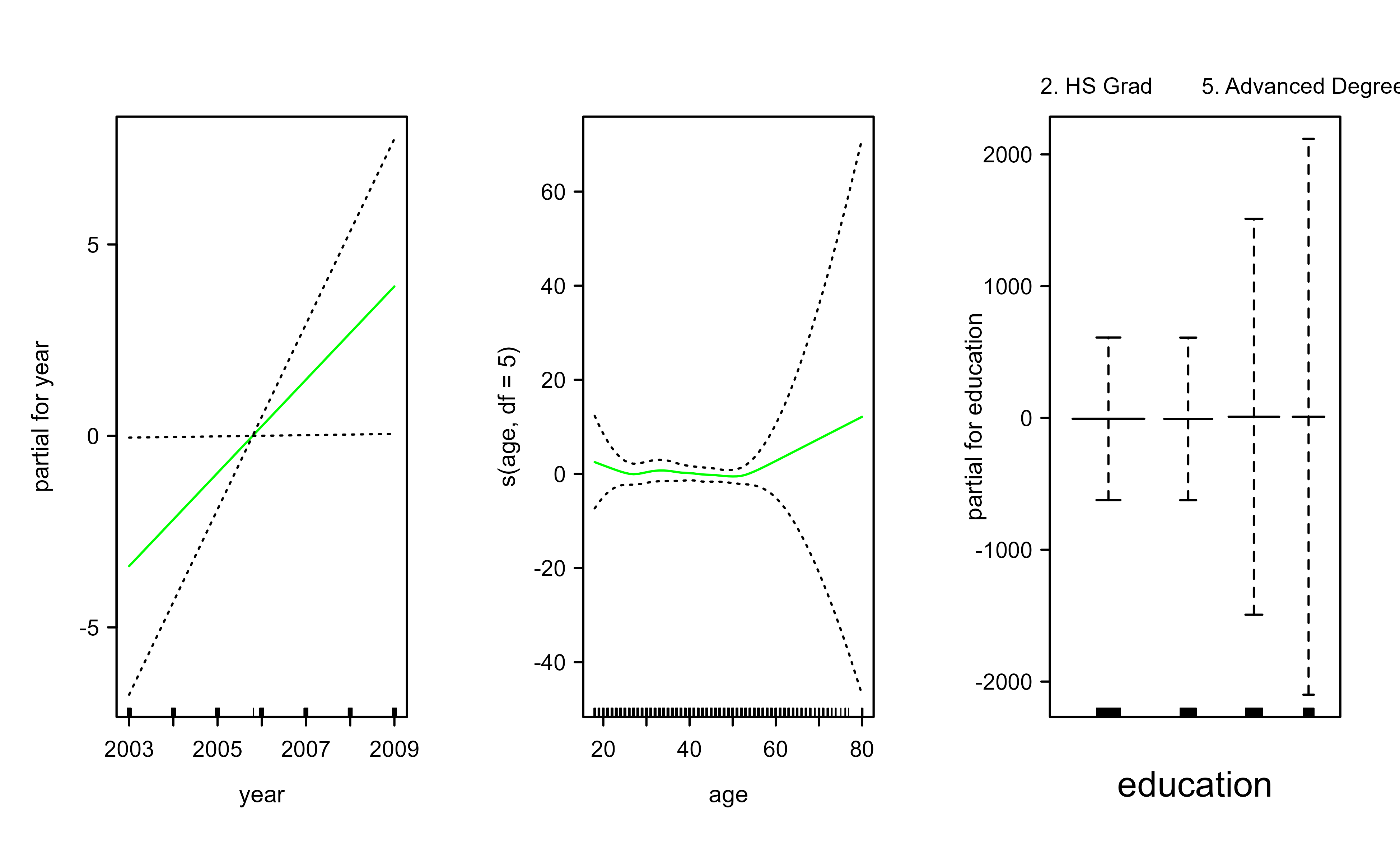
The additive idea extends to a binary outcome through a logistic link. Figure 6.5 fits a logistic GAM for the indicator that wage exceeds 250.

if ("package:mgcv" %in% search()) detach("package:mgcv")
gam.lr <- gam(I(wage > 250) ~ year + s(age, df = 5) + education,
              family = binomial,
              data = Wage)
par(mfrow = c(1, 3))
plot(gam.lr, se = T, col = "green")

Figure 6.5: Components of a logistic GAM for the probability that wage exceeds 250, with a linear year term and a smooth age term.

Table 6.2 cross-tabulates education against the high-wage indicator, which motivates dropping the sparse lowest education level before refitting.

knitr::kable(
  table(Wage$education, I(Wage$wage > 25)),
  caption = "Cross-tabulation of education level against the indicator that wage exceeds 25."
)

Table 6.2: Cross-tabulation of education level against the indicator that wage exceeds 25.

	FALSE	TRUE
1. < HS Grad	1	267
2. HS Grad	2	969
3. Some College	3	647
4. College Grad	0	685
5. Advanced Degree	0	426

Figure 6.6 refits the logistic GAM after excluding the lowest education category.

if ("package:mgcv" %in% search()) detach("package:mgcv")
gam.lr.s <- gam(
    I(wage > 25) ~ year + s(age, df = 5) + education,
    family = binomial,
    data = Wage,
    subset = (education != "1. < HS Grad")
)
par(mfrow = c(1, 3))
plot(gam.lr.s, se = T, col = "green")

Figure 6.6: Logistic GAM for the high-wage indicator after excluding the lowest education category, which removes the unstable estimates caused by its empty cell.

6.6.2 Example 2

Spline regression makes you choose where to place the knots by hand. To sidestep spline regression’s (Chapter 3) requirement for specifying the knots, we can use a GAM, which selects the smoothness automatically through its penalty. Here we fit a single smooth of medv on lstat with mgcv and check how well it generalizes to a held-out test set.

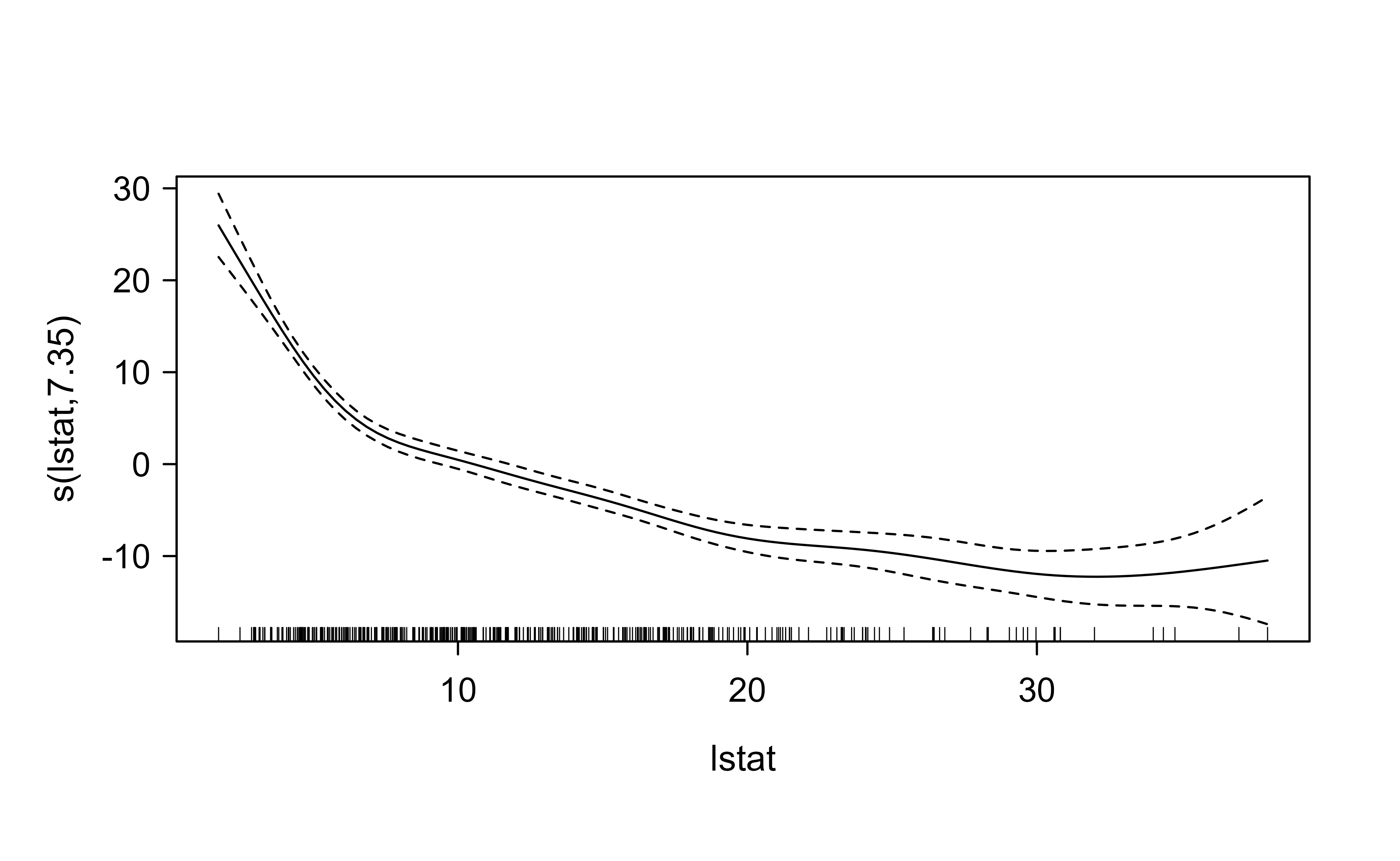
Figure 6.7 shows the estimated smooth term, and Table 6.3 reports its accuracy on the held-out test set.

library(tidyverse)
library(caret)
# Load the data
data("Boston", package = "MASS")
# Split the data into training and test set
set.seed(123)
training.samples <- Boston$medv %>%
    caret::createDataPartition(p = 0.8, list = FALSE)
train.data  <- Boston[training.samples,]
test.data <- Boston[-training.samples,]

attach(train.data)

library(mgcv)
# Build the model
model <- gam(medv ~ s(lstat), data = train.data)
plot(model)

Figure 6.7: Estimated smooth effect of lstat on the median home value medv from an mgcv GAM fitted on the Boston training set, with a pointwise standard-error band.

# Make predictions
predictions <- model %>% predict(test.data)
# Model performance
knitr::kable(
  data.frame(
    RMSE = RMSE(predictions, test.data$medv),
    R2 = R2(predictions, test.data$medv)
  ),
  caption = "Test-set root-mean-squared error and R-squared for the Boston GAM with a single smooth of lstat."
)

Table 6.3: Test-set root-mean-squared error and R-squared for the Boston GAM with a single smooth of lstat.

RMSE	R2
5.318856	0.6760512

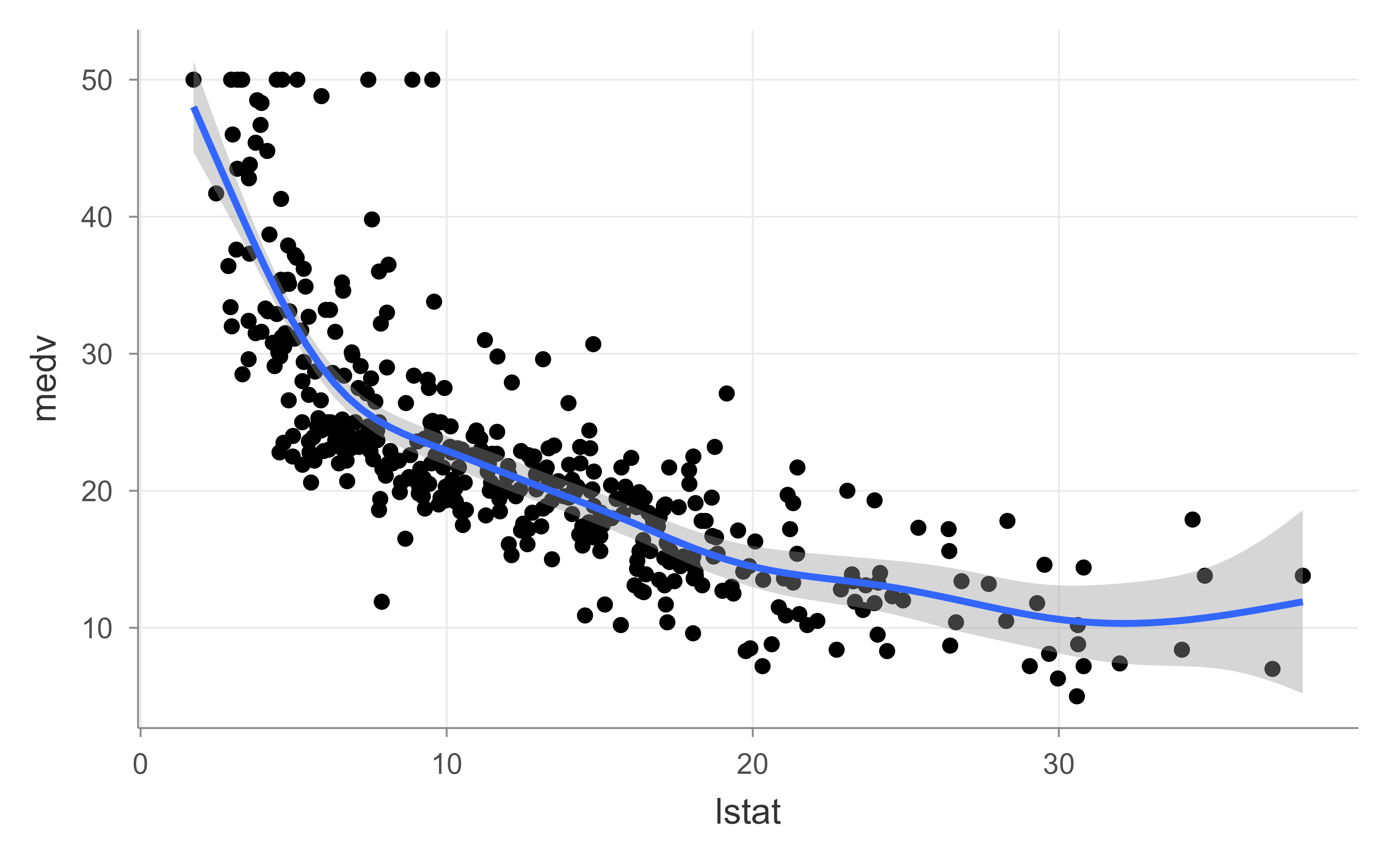
Figure 6.8 overlays the same smooth on the training scatterplot using stat_smooth.

ggplot(train.data, aes(lstat, medv) ) +
  geom_point() +
  stat_smooth(method = gam, formula = y ~ s(x))
detach(train.data)

Figure 6.8: Training-set scatterplot of medv against lstat with an overlaid GAM smooth fitted through stat_smooth, showing the same curved relationship as the mgcv fit.

The fitted curve bends sharply where lstat is low and flattens as lstat grows, a nonlinearity that a single straight line would miss entirely, and the test-set \(R^2\) in Table 6.3 quantifies how much of that signal carries over to new data. Notice that we never told mgcv how many knots to use or where to put them: the penalty did that work for us, which is the practical payoff of the smoothness criterion from the start of this chapter.

Hastie, Trevor, Jerome Friedman, and Robert Tibshirani. 2001. The Elements of Statistical Learning. Springer New York. https://doi.org/10.1007/978-0-387-21606-5.

James, Gareth, Daniela Witten, Trevor Hastie, and Robert Tibshirani. 2013. “Statistical Learning.” In, 15–57. Springer New York. https://doi.org/10.1007/978-1-4614-7138-7_2.

---

1. Unspecified means we do not commit to a parametric form like \(\beta_j X_j\) or \(\beta_j X_j^2\) in advance. We let the data choose the shape of each curve, subject to a smoothness penalty introduced later.

2. This is the same smoothness penalty used for a single smoothing spline (Chapter 3). A GAM simply applies it once per predictor and ties the pieces together additively.

3. https://highstat.com/index.php/beginner-s-guide-to-generalized-additive-models-with-r