74 Hidden Markov Models
Suggested reading:
Many data sets arrive as a sequence: a stretch of text read one word at a time, a recording sampled every few milliseconds, a patient observed across weekly visits, a financial index quoted each trading day. Two features set sequential data apart from the independent and identically distributed observations that most of this book has assumed. First, neighbouring observations are correlated, so treating them as independent throws away information. Second, the thing we actually care about is often not the observation itself but a hidden state that produced it: the part of speech that generated a word, the physiological regime that produced a heartbeat, the market mood that produced a price move. A hidden Markov model (HMM) is the simplest probabilistic model that takes both features seriously.
The intuition is worth stating in plain language before any algebra. Picture a system that moves through a small set of internal states over time, hopping from one to the next according to fixed probabilities, with no memory of how it got there beyond its current state. We never see the states. What we see instead, at each time step, is a noisy signal whose distribution depends only on the current hidden state. The classic teaching example is the occasionally dishonest casino: a dealer secretly switches between a fair die and a loaded one, and all we observe is the stream of rolls. The dealer’s choice of die is the hidden state; the roll is the observation. Our job is to reason backwards from the rolls to questions like “how likely is this whole sequence of rolls under the casino’s scheme?”, “when was the loaded die in play?”, and “what switching and loading probabilities best explain what we saw?”
Those three questions are not casual. They are the three canonical problems of HMMs, and essentially all of the theory is machinery for answering them efficiently. The naive answer to the first (“sum over all possible state sequences”) costs an amount of work that grows exponentially in the length of the sequence, which is hopeless. The contribution of the HMM literature is a set of dynamic-programming recursions, the forward-backward and Viterbi algorithms, that reduce the cost to linear in the sequence length. This chapter develops those recursions from scratch, derives the Baum-Welch expectation-maximization procedure that learns the parameters, places HMMs in the wider family of latent-variable and graphical models (linking them to mixture models from Chapter 23, to Kalman filters, and to the discriminative conditional random fields of Chapter 77), and closes with a base-R implementation on the dishonest casino that you can run and check.
Key idea
An HMM couples a latent Markov chain (the states, which we never see) to an observation model (the emissions, which we do see). Every useful computation reduces to a dynamic-programming recursion over time that replaces an exponential sum or maximization with a linear-time one.
74.1 The Model as a Temporal Graphical Model
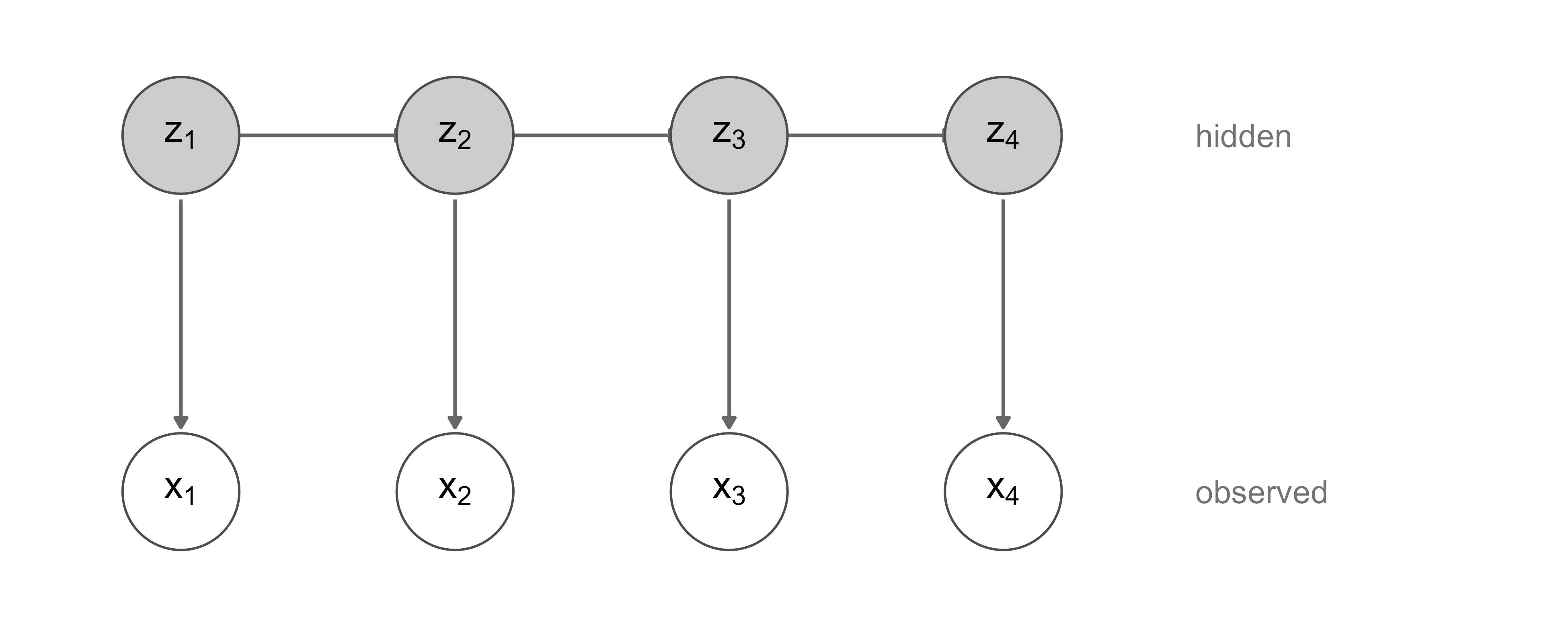
We observe a sequence \(\mathbf{x}_{1:T} = (x_1, x_2, \dots, x_T)\). Behind it sits an unobserved sequence of states \(\mathbf{z}_{1:T} = (z_1, \dots, z_T)\), where each \(z_t\) takes one of \(K\) discrete values, written \(z_t \in \{1, \dots, K\}\). The model is built from two conditional-independence assumptions, and almost everything that follows is a consequence of them.
The first assumption is the (first-order) Markov property on the hidden chain: the next state depends on the present state and nothing earlier,
\[ p(z_t \mid z_{1:t-1}) = p(z_t \mid z_{t-1}). \tag{74.1}\]
The second is the emission (output) independence: each observation depends only on the state active at that same time,
\[ p(x_t \mid z_{1:t}, x_{1:t-1}) = p(x_t \mid z_t). \tag{74.2}\]
Together these factorize the joint distribution of states and observations into a clean product of local terms,
\[ p(\mathbf{z}_{1:T}, \mathbf{x}_{1:T}) = p(z_1) \prod_{t=2}^{T} p(z_t \mid z_{t-1}) \prod_{t=1}^{T} p(x_t \mid z_t). \tag{74.3}\]
Read as a graphical model, an HMM is a chain: the latent nodes \(z_1 \to z_2 \to \cdots \to z_T\) form a Markov backbone, and each \(z_t\) emits a single observed child \(x_t\) hanging off it. This is exactly the structure shown in Figure 74.1. Because the graph is a tree (no undirected cycles), exact inference is tractable, which is the deep reason the linear-time recursions exist at all.
74.1.1 Parameters
An HMM with \(K\) states is specified by three sets of parameters, collectively written \(\theta = (\boldsymbol{\pi}, \mathbf{A}, \mathbf{B})\).
The initial distribution \(\boldsymbol{\pi}\), a length-\(K\) vector with \(\pi_i = p(z_1 = i)\), giving the probability of starting in each state.
The transition matrix \(\mathbf{A}\), a \(K \times K\) stochastic matrix with entries \(A_{ij} = p(z_t = j \mid z_{t-1} = i)\), the probability of moving from state \(i\) to state \(j\). Each row sums to one.
The emission model \(\mathbf{B}\), the family of conditional distributions \(p(x_t \mid z_t = i)\). When observations are discrete with \(M\) possible symbols, \(\mathbf{B}\) is a \(K \times M\) matrix with \(B_{ik} = p(x_t = k \mid z_t = i)\), and each row sums to one. When observations are continuous, the rows are replaced by densities, for example a Gaussian \(\mathcal{N}(\mu_i, \sigma_i^2)\) per state.
A mixture model with memory
If you delete the transition structure (force \(A_{ij} = \pi_j\) so the state is redrawn independently each step) the HMM collapses to a finite mixture model: each \(x_t\) is drawn from one of \(K\) component distributions chosen at random. The HMM is therefore a mixture model whose component-selection variable carries Markov memory across time. This is the cleanest way to connect it to the clustering and mixture material in Chapter 23.
74.2 The Three Canonical Problems
Rabiner’s classic tutorial organizes the entire subject around three problems, and it pays to name them up front because the algorithms map onto them one for one.
Evaluation (likelihood). Given parameters \(\theta\) and an observed sequence \(\mathbf{x}_{1:T}\), compute the likelihood \(p(\mathbf{x}_{1:T} \mid \theta)\). Solved by the forward algorithm.
Decoding. Given \(\theta\) and \(\mathbf{x}_{1:T}\), find the single most probable hidden path \(\mathbf{z}_{1:T}^\star = \arg\max_{\mathbf{z}_{1:T}} p(\mathbf{z}_{1:T} \mid \mathbf{x}_{1:T}, \theta)\). Solved by the Viterbi algorithm.
Learning. Given only observations (and the number of states \(K\)), estimate \(\theta\) by maximizing \(p(\mathbf{x}_{1:T} \mid \theta)\). Solved by the Baum-Welch algorithm, an instance of expectation-maximization.
The next three sections take these in turn.
74.3 Evaluation: the Forward-Backward Algorithm
The likelihood is obtained, in principle, by summing the joint distribution Equation 74.3 over all hidden paths,
\[ p(\mathbf{x}_{1:T}) = \sum_{\mathbf{z}_{1:T}} p(\mathbf{z}_{1:T}, \mathbf{x}_{1:T}). \tag{74.4}\]
There are \(K^T\) paths, so this brute-force sum is intractable for any realistic \(T\). The escape is to push the sum inside the product and reuse partial results, which is exactly dynamic programming.
74.3.1 The forward recursion
Define the forward variable as the joint probability of the observations up to time \(t\) together with the state at time \(t\),
\[ \alpha_t(i) = p(x_{1:t}, z_t = i). \tag{74.5}\]
We derive a recursion for it. At \(t = 1\), the definition and the factorization give the base case directly,
\[ \alpha_1(i) = p(x_1, z_1 = i) = \pi_i \, p(x_1 \mid z_1 = i). \tag{74.6}\]
For the inductive step, write \(\alpha_{t+1}(j)\) and condition on the previous state by marginalizing over it,
\[ \begin{aligned} \alpha_{t+1}(j) &= p(x_{1:t+1}, z_{t+1} = j) \\ &= \sum_{i=1}^{K} p(x_{1:t}, z_t = i, z_{t+1} = j, x_{t+1}). \end{aligned} \tag{74.7}\]
Now apply the chain rule to the summand and drop terms that the conditional-independence assumptions Equation 74.1 and Equation 74.2 make irrelevant. The factor \(z_{t+1}\) depends on the past only through \(z_t\), and \(x_{t+1}\) depends only on \(z_{t+1}\), so
\[ \begin{aligned} p(x_{1:t}, z_t = i, z_{t+1} = j, x_{t+1}) &= \underbrace{p(x_{1:t}, z_t = i)}_{\alpha_t(i)} \\ &\quad\times \underbrace{p(z_{t+1} = j \mid z_t = i)}_{A_{ij}} \\ &\quad\times \underbrace{p(x_{t+1} \mid z_{t+1} = j)}_{b_j(x_{t+1})}. \end{aligned} \tag{74.8}\]
Substituting back yields the forward recursion, which advances the joint probability one step at a time,
\[ \alpha_{t+1}(j) = b_j(x_{t+1}) \sum_{i=1}^{K} \alpha_t(i)\, A_{ij}, \tag{74.9}\]
where \(b_j(x) = p(x \mid z = j)\) is the emission probability. Once the recursion reaches \(t = T\), the likelihood is recovered by marginalizing the final state,
\[ p(\mathbf{x}_{1:T}) = \sum_{i=1}^{K} \alpha_T(i). \tag{74.10}\]
Each step costs \(O(K^2)\) work (a matrix-vector product), repeated \(T\) times, so the total cost is \(O(K^2 T)\): linear in the sequence length, a colossal improvement over the \(O(K^T)\) brute-force sum.
74.3.2 The backward recursion
A symmetric quantity proves indispensable for learning. Define the backward variable as the probability of the future observations given the current state,
\[ \beta_t(i) = p(x_{t+1:T} \mid z_t = i), \tag{74.11}\]
with the convention \(\beta_T(i) = 1\) for all \(i\) (there is no future to condition on at the last step). By the same conditioning argument run in reverse, marginalizing over the next state \(z_{t+1} = j\),
\[ \beta_t(i) = \sum_{j=1}^{K} A_{ij}\, b_j(x_{t+1})\, \beta_{t+1}(j). \tag{74.12}\]
Combining the two sweeps, the smoothed posterior probability that the chain occupied state \(i\) at time \(t\), given the entire sequence, follows from Bayes’ rule because \(\alpha_t(i)\beta_t(i) = p(x_{1:t}, z_t=i)\,p(x_{t+1:T}\mid z_t=i) = p(\mathbf{x}_{1:T}, z_t=i)\),
\[ \gamma_t(i) = p(z_t = i \mid \mathbf{x}_{1:T}) = \frac{\alpha_t(i)\,\beta_t(i)}{\sum_{k=1}^{K} \alpha_t(k)\,\beta_t(k)}. \tag{74.13}\]
The vector \(\gamma_t\) answers the question “given everything I observed, where was the chain at time \(t\)?”, and its entries are precisely the per-time posterior over states that we will use both for soft decoding and for the M-step of learning.
74.3.3 Scaling for numerical stability
The forward variables are joint probabilities of ever-longer observation sequences, so they shrink roughly geometrically and underflow to zero in double precision within a few hundred steps. The standard cure is to rescale at every step. Define the normalizer \(c_t\) and the scaled forward variable \(\hat\alpha_t\) by
\[ c_t = \sum_{i=1}^{K} b_i(x_t) \sum_{j} \hat\alpha_{t-1}(j) A_{ji}, \qquad \hat\alpha_t(i) = \frac{1}{c_t}\, b_i(x_t) \sum_{j} \hat\alpha_{t-1}(j) A_{ji}, \tag{74.14}\]
so that \(\sum_i \hat\alpha_t(i) = 1\) at every \(t\). The scaling constant \(c_t\) turns out to equal the one-step predictive likelihood \(p(x_t \mid x_{1:t-1})\), and therefore the full log-likelihood is recovered by summing the logs of the normalizers,
\[ \log p(\mathbf{x}_{1:T}) = \sum_{t=1}^{T} \log c_t. \tag{74.15}\]
This is the form to implement in practice: it keeps every quantity in a sane numerical range and delivers the log-likelihood directly. (Viterbi sidesteps the issue differently, by working in log space throughout, as we see next.)
Why a product of normalizers gives the likelihood
Telescoping the chain rule, \(p(\mathbf{x}_{1:T}) = \prod_t p(x_t \mid x_{1:t-1})\). Each scaling constant \(c_t\) is exactly one of these one-step factors, so their product is the joint likelihood and the sum of their logs is the log-likelihood. Scaling is not a hack bolted on for stability; it is the likelihood, factored.
74.4 Decoding: the Viterbi Algorithm
The forward algorithm sums over paths. If we instead want the single most probable path, we replace every sum with a maximum and keep backpointers so we can reconstruct the winner. Define
\[ \delta_t(i) = \max_{z_{1:t-1}} p(z_{1:t-1}, z_t = i, x_{1:t}), \tag{74.16}\]
the probability of the best path that ends in state \(i\) at time \(t\). The base case mirrors the forward one, \(\delta_1(i) = \pi_i\, b_i(x_1)\). The recursion is identical to Equation 74.9 with the sum turned into a max,
\[ \delta_{t+1}(j) = b_j(x_{t+1}) \max_{i} \big[\delta_t(i)\, A_{ij}\big], \tag{74.17}\]
and we store the maximizing predecessor at each step,
\[ \psi_{t+1}(j) = \arg\max_{i} \big[\delta_t(i)\, A_{ij}\big]. \tag{74.18}\]
At \(t = T\) the best final state is \(z_T^\star = \arg\max_i \delta_T(i)\), and we trace the backpointers backwards, \(z_t^\star = \psi_{t+1}(z_{t+1}^\star)\), to recover the whole optimal path. The cost is again \(O(K^2 T)\).
In practice the products underflow just as the forward variables do, so Viterbi is run in log space, where products become sums and the max is preserved by the monotone log,
\[ \log \delta_{t+1}(j) = \log b_j(x_{t+1}) + \max_{i}\big[\log \delta_t(i) + \log A_{ij}\big]. \tag{74.19}\]
Viterbi path versus posterior marginals
The Viterbi path is the single most probable joint state sequence. The sequence of per-time posterior modes, \(\hat z_t = \arg\max_i \gamma_t(i)\) from Equation 74.13, maximizes the expected number of individually correct states instead. These two answers can differ, and the marginal-mode path can even include a transition the model forbids (\(A_{ij} = 0\)), because nothing constrains it to be a legal path. Use Viterbi when you need a coherent trajectory; use the marginals when you care about per-time-point accuracy.
74.5 Learning: the Baum-Welch (EM) Algorithm
When the parameters are unknown we cannot maximize the likelihood Equation 74.10 directly, because it is a sum over hidden paths and the logarithm does not pass through the sum. The Baum-Welch algorithm resolves this with expectation-maximization: it alternates between computing the expected hidden statistics under the current parameters (the E-step, which is just forward-backward) and re-estimating the parameters from those expectations in closed form (the M-step).
74.5.1 The E-step quantities
Beyond the smoothed state posterior \(\gamma_t(i)\) of Equation 74.13, learning needs the joint posterior over consecutive state pairs, the expected transition usage,
\[ \xi_t(i,j) = p(z_t = i, z_{t+1} = j \mid \mathbf{x}_{1:T}) = \frac{\alpha_t(i)\, A_{ij}\, b_j(x_{t+1})\, \beta_{t+1}(j)}{p(\mathbf{x}_{1:T})}. \tag{74.20}\]
The numerator is precisely the four factors that make up a single transition: how we got to state \(i\) (the \(\alpha\)), the transition itself (\(A_{ij}\)), the emission it produces (\(b_j\)), and how the future unfolds from \(j\) (the \(\beta\)).
74.5.2 The M-step updates
Given the expected counts, the parameter updates are the intuitive normalized tallies, and each can be derived as the exact maximizer of the EM auxiliary function (the expected complete-data log-likelihood) subject to the stochastic constraints, using one Lagrange multiplier per row. The initial distribution is the expected state occupancy at time one,
\[ \hat\pi_i = \gamma_1(i). \tag{74.21}\]
Each transition probability is the expected number of \(i \to j\) transitions divided by the expected number of departures from \(i\),
\[ \hat A_{ij} = \frac{\sum_{t=1}^{T-1} \xi_t(i,j)}{\sum_{t=1}^{T-1} \gamma_t(i)}. \tag{74.22}\]
For discrete emissions, each emission probability is the expected number of times state \(i\) emitted symbol \(k\) divided by the expected number of visits to \(i\),
\[ \hat B_{ik} = \frac{\sum_{t=1}^{T} \gamma_t(i)\, \mathbb{1}[x_t = k]}{\sum_{t=1}^{T} \gamma_t(i)}. \tag{74.23}\]
For Gaussian emissions, the same logic gives \(\gamma\)-weighted means and variances per state, exactly as in a Gaussian mixture but with the responsibilities supplied by forward-backward instead of by an independent posterior.
Why this converges, and to what
Baum-Welch is EM, so each iteration cannot decrease the observed-data likelihood (the E-step builds a tight lower bound at the current parameters; the M-step maximizes it). For discrete emissions the likelihood is a probability bounded above by one, so the monotonically non-decreasing sequence converges. For continuous (for example Gaussian) emissions the likelihood is a density and can be unbounded; Baum-Welch still increases it monotonically but can drift toward a degenerate solution (a state variance collapsing to zero), which is why variance floors or priors are used in practice. The fixed point is a stationary point of the likelihood, typically a local maximum, never guaranteed to be the global one. The likelihood surface is also invariant to relabeling the states (label switching), so it has at least \(K!\) equivalent maxima.
Practical failure modes
Three issues bite repeatedly. (1) Local optima: run from several random initializations and keep the best log-likelihood. (2) Zero counts: a symbol never emitted in a state drives \(\hat B_{ik}\) to zero, which then makes any future sequence containing that pair impossible; add a small Laplace/Dirichlet smoothing constant, mirroring the same fix in Chapter 18. (3) Choosing \(K\): the likelihood always rises with more states, so select \(K\) by a penalized criterion (AIC/BIC) or held-out likelihood, not by training fit.
74.6 Connections to Other Models
The HMM sits at a busy crossroads, and seeing the neighbours sharpens what it is.
Kalman filters (continuous latent state). Replace the discrete state \(z_t\) with a continuous Gaussian state and make both the transition and emission linear-Gaussian, and the model becomes a linear dynamical system. The forward algorithm’s exact analogue is the Kalman filter; the forward-backward smoother becomes the Kalman (Rauch-Tung-Striebel) smoother. The recursions are the same dynamic program, but because everything is Gaussian the “sum over states” becomes an integral that stays Gaussian in closed form, so we propagate a mean and covariance rather than a discrete distribution. The Gaussian machinery here is the same conditioning identity that powers Chapter 7.
Conditional random fields (discriminative analogue). An HMM is a generative model: it specifies the joint \(p(\mathbf{z}, \mathbf{x})\) and spends modeling effort on \(p(\mathbf{x} \mid \mathbf{z})\). A linear-chain conditional random field keeps the same chain structure but models the conditional \(p(\mathbf{z} \mid \mathbf{x})\) directly, with feature functions that may depend on the whole observation sequence at once and need not be normalized per state. The chapter on Chapter 77 develops CRFs in full; the short version is that CRFs trade the HMM’s generative story (and its ability to handle missing inputs) for the freedom to use rich, overlapping features of the input, which usually helps when the goal is purely to label sequences.
Mixture models and neural sequence models. As noted above, an HMM with the transition structure removed is a finite mixture (Chapter 23). In the other direction, replacing the fixed emission and transition tables with neural networks, and the discrete state with a high-dimensional continuous one, leads toward recurrent networks and the attention-based sequence models of Chapter 38; an HMM is, in a sense, the fully probabilistic and exactly-inferable ancestor of those models.
74.7 Practical Guidance
A few rules of thumb carry most of the practical weight.
Always scale or work in logs. Unscaled forward variables underflow within a few hundred steps. Use Equation 74.15 for the likelihood and Equation 74.19 for decoding.
Initialize sensibly. Random restarts beat a single run. For Gaussian emissions, seeding state means with a k-means pass (Chapter 23) is a strong default.
Smooth the estimates. Add a small pseudocount to emission and transition counts to avoid the zero-probability trap, especially with short sequences or many symbols.
Choose \(K\) honestly. Use BIC or held-out likelihood. Constrain \(\mathbf{A}\) (for example, left-to-right topologies in speech) when domain knowledge justifies it; fewer free parameters means more stable estimates.
Match the decoder to the question. Viterbi for a coherent path, \(\gamma_t\) marginals for per-step labels and for honest uncertainty.
When you need full posterior uncertainty over parameters rather than a point estimate, the Bayesian treatment (placing Dirichlet priors on the rows and sampling with forward-filtering backward-sampling) is a natural next step and connects to the tooling in Chapter 75.
74.8 R Demonstration: the Occasionally Dishonest Casino
We now implement the forward (with scaling) and Viterbi (in log space) algorithms from scratch in base R and verify them on the dishonest-casino HMM. The casino has two states, fair (\(F\)) and loaded (\(L\)). The fair die is uniform over \(\{1,\dots,6\}\); the loaded die rolls a six with probability \(0.5\) and the other faces with probability \(0.1\) each. The dealer tends to stick with the current die (high self-transition probabilities). We simulate a sequence with known hidden states, then check three things: that our scaled forward log-likelihood matches an independent brute-force sum over all paths (on a short sequence), that the Viterbi path recovers the true regime well, and that the decoded structure looks sensible.
Show code
set.seed(123)

## --- model parameters (theta) ------------------------------------------
states <- c("Fair", "Loaded")
K <- 2L
pi0 <- c(Fair = 0.5, Loaded = 0.5)                 # initial distribution
A <- matrix(c(0.95, 0.05,                            # P(.|Fair)
              0.10, 0.90),                           # P(.|Loaded)
            nrow = 2, byrow = TRUE,
            dimnames = list(states, states))
## emission matrix B[state, face], faces 1..6
B <- rbind(Fair   = rep(1/6, 6),
           Loaded = c(0.1, 0.1, 0.1, 0.1, 0.1, 0.5))
colnames(B) <- 1:6

## --- simulate a sequence with known hidden states ----------------------
simulate_hmm <- function(Tlen, pi0, A, B) {
  z <- integer(Tlen); x <- integer(Tlen)
  z[1] <- sample(K, 1, prob = pi0)
  x[1] <- sample(6, 1, prob = B[z[1], ])
  for (t in 2:Tlen) {
    z[t] <- sample(K, 1, prob = A[z[t - 1], ])
    x[t] <- sample(6, 1, prob = B[z[t], ])
  }
  list(z = z, x = x)
}
Tlen <- 300L
sim <- simulate_hmm(Tlen, pi0, A, B)

## --- forward algorithm with scaling ------------------------------------
forward_scaled <- function(x, pi0, A, B) {
  Tlen <- length(x); K <- nrow(A)
  alpha <- matrix(0, Tlen, K); cscale <- numeric(Tlen)
  a <- pi0 * B[, x[1]]                 # unnormalized alpha_1
  cscale[1] <- sum(a)
  alpha[1, ] <- a / cscale[1]
  for (t in 2:Tlen) {
    a <- (alpha[t - 1, ] %*% A) * B[, x[t]]  # vector of length K
    cscale[t] <- sum(a)
    alpha[t, ] <- a / cscale[t]
  }
  list(alpha = alpha, cscale = cscale,
       loglik = sum(log(cscale)))
}
fwd <- forward_scaled(sim$x, pi0, A, B)

## --- brute-force likelihood on a SHORT sequence (verification) ---------
brute_force_loglik <- function(x, pi0, A, B) {
  Tlen <- length(x); K <- nrow(A)
  paths <- expand.grid(rep(list(1:K), Tlen))   # all K^T state paths
  total <- 0
  for (r in seq_len(nrow(paths))) {
    z <- as.integer(paths[r, ])
    p <- pi0[z[1]] * B[z[1], x[1]]
    for (t in 2:Tlen) p <- p * A[z[t - 1], z[t]] * B[z[t], x[t]]
    total <- total + p
  }
  log(total)
}
short <- sim$x[1:8]
ll_fwd_short   <- forward_scaled(short, pi0, A, B)$loglik
ll_brute_short <- brute_force_loglik(short, pi0, A, B)

## --- Viterbi in log space ----------------------------------------------
viterbi_log <- function(x, pi0, A, B) {
  Tlen <- length(x); K <- nrow(A)
  lA <- log(A); lB <- log(B); lpi <- log(pi0)
  delta <- matrix(-Inf, Tlen, K); psi <- matrix(0L, Tlen, K)
  delta[1, ] <- lpi + lB[, x[1]]
  for (t in 2:Tlen) {
    for (j in 1:K) {
      scores <- delta[t - 1, ] + lA[, j]
      psi[t, j] <- which.max(scores)
      delta[t, j] <- max(scores) + lB[j, x[t]]
    }
  }
  z <- integer(Tlen)
  z[Tlen] <- which.max(delta[Tlen, ])
  for (t in (Tlen - 1):1) z[t] <- psi[t + 1, z[t + 1]]
  list(path = z, logprob = max(delta[Tlen, ]))
}
vit <- viterbi_log(sim$x, pi0, A, B)

## --- report -------------------------------------------------------------
cat(sprintf("Scaled forward log-likelihood (T=%d): %.4f\n", Tlen, fwd$loglik))
#> Scaled forward log-likelihood (T=300): -512.3911
cat(sprintf("Verification on T=8 -> forward: %.6f | brute force: %.6f | diff: %.2e\n",
            ll_fwd_short, ll_brute_short, abs(ll_fwd_short - ll_brute_short)))
#> Verification on T=8 -> forward: -14.981317 | brute force: -14.981317 | diff: 1.78e-15
decode_acc <- mean(vit$path == sim$z)
cat(sprintf("Viterbi decoding accuracy vs. true states: %.1f%%\n", 100 * decode_acc))
#> Viterbi decoding accuracy vs. true states: 72.0%
The forward log-likelihood computed with scaling matches the independent brute-force sum on the short sequence to within floating-point precision, which confirms the recursion Equation 74.9 and the scaled-likelihood identity Equation 74.15 are implemented correctly. The Viterbi path recovers most of the true fair-versus-loaded regime, with errors concentrated near the switch points where even an optimal decoder is genuinely uncertain (the loaded die only mildly biases the rolls, so short loaded runs are inherently hard to distinguish from chance).
Finally, Figure 74.2 overlays the true hidden regime, the observed rolls, and the Viterbi decoding, making the model’s behaviour visible: stretches dominated by sixes are decoded as loaded, and the decoder smooths over isolated rolls because the high self-transition probabilities penalize rapid switching.
Show code
library(ggplot2)
df <- data.frame(
  t       = seq_len(Tlen),
  roll    = sim$x,
  true    = factor(states[sim$z], levels = states),
  decoded = factor(states[vit$path], levels = states)
)
df$true_num    <- ifelse(df$true == "Loaded", 1, 0)
df$decoded_num <- ifelse(df$decoded == "Loaded", 1, 0)

p_top <- ggplot(df, aes(t, roll, colour = true)) +
  geom_point(size = 1.3) +
  scale_colour_manual(values = c(Fair = "grey45", Loaded = "firebrick"),
                      name = "True state") +
  labs(x = NULL, y = "Die roll") +
  theme_book()

p_bot <- ggplot(df, aes(t)) +
  geom_area(aes(y = true_num), fill = "grey85") +
  geom_line(aes(y = decoded_num), colour = "firebrick", linewidth = 0.6) +
  scale_y_continuous(breaks = c(0, 1), labels = c("Fair", "Loaded")) +
  labs(x = "Time (roll index)", y = "Regime",
       subtitle = "Band: true regime   Line: Viterbi decoding") +
  theme_book()

## stack the two panels without extra packages
gridExtra::grid.arrange(p_top, p_bot, heights = c(1, 1))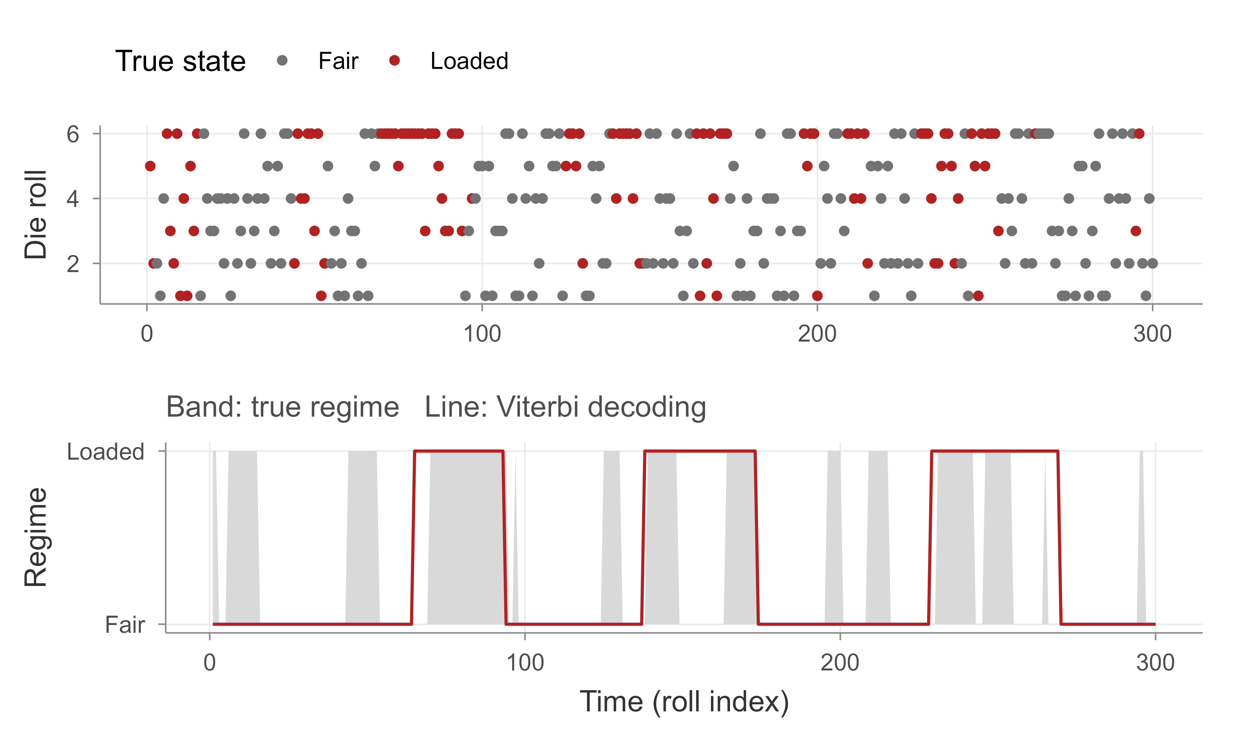
To go further, the same forward_scaled and a matching backward pass give the \(\gamma_t\) posteriors of Equation 74.13 (soft decoding), and wrapping the E-step counts Equation 74.13 and Equation 74.20 inside the M-step updates Equation 74.21 to Equation 74.23 yields a full Baum-Welch learner that recovers \(\mathbf{A}\) and \(\mathbf{B}\) from the rolls alone. For production work the depmixS4 and HMM packages implement all of this (with multiple sequences, covariate-dependent transitions, and several emission families) and are the sensible tools once the mechanics above are understood.