Most real data does not live in a .csv file on your laptop. It lives in a database: a transactional store behind an application, a data warehouse, or an analytical engine that someone else maintains. A data scientist, analyst, or ML engineer who can only work with data after it has been exported to a flat file is limited to whatever someone else chose to export. The skill this chapter builds is the ability to pull exactly the rows and columns you need, computed where the data already sits, and bring only the result into R.
The chapter covers the standard R interface to databases (DBI), how to write safe parameterized queries, and how dbplyr lets you write ordinary dplyr code that is translated into SQL and run inside the database. The mathematical content is the relational model and its algebra, which is what SQL is a syntax for. By the end you should be able to connect to a database from R, push filtering and aggregation into the engine, pull back only the small result you need, and recognize the safety and performance traps that bite people in production.
Key idea
The single most consequential choice in a data pipeline is where the computation happens. Doing the work in the database and shipping a small answer to R is usually faster, cheaper, and safer than shipping a huge table to R and working on it there.
Because the database packages (DBI, RSQLite, dbplyr, duckdb) are outside the set of packages this book runs at build time, those chunks are marked eval=FALSE; they are correct, current code you can run.1 A self-contained base R demonstration at the end teaches the same ideas with no external dependency, so you can see every concept run even without a database.
99.1 Where this fits in a modern ML and AI workflow
A typical pipeline starts with raw data in a database and ends with a model or an analysis. The decision you make at the very first step, how much computation to push into the database versus pull into R, often dominates the runtime and the memory footprint of everything downstream.
The principle is to do filtering, joining, and aggregation in the database, where the data already lives and where indexes and query planners exist, and to bring into R only the comparatively small, already-reduced table that you will model on. Pulling a billion-row table into R to then keep ten thousand rows is the most common and most expensive mistake.
Intuition
Think of the database as a warehouse and R as your workbench. You do not haul the entire warehouse to your bench to find one box; you ask the warehouse to find the box and send it over. The “asking” is SQL, and the box is the result of your query.
[ database ] --SQL/dbplyr--> [ filtered, joined, aggregated result ] --collect()--> [ R data frame ] --> [ recipe / model / plot ]
This pattern appears everywhere in practice: assembling a feature table for a model by joining several source tables, computing label definitions with window functions, sampling a class-balanced training set with a stratified query, or scoring new records by reading them in batches. The same DBI connection object is also what monitoring code (Chapter 117), scheduled jobs, and feature stores (Chapter 119) use.
99.2 The relational model and relational algebra
Before touching any package, it helps to know what SQL actually is. SQL is a concrete syntax for relational algebra, a small mathematical language for transforming tables. You do not need the algebra to write queries, but knowing it makes the translation that dbplyr performs predictable: once you can see a dplyr pipeline as a sequence of algebra operators, you can predict the SQL it will generate and reason about why one ordering of steps runs faster than another.
A relation (the formal name for a table) is a set of tuples (rows) drawn from a Cartesian product of attribute domains (columns).2 Write a relation \(R\) with attributes \(A_1, \dots, A_k\) as a subset \[
R \subseteq D_1 \times D_2 \times \cdots \times D_k,
\] where \(D_j\) is the domain (the set of allowed values) of attribute \(A_j\). Each element of \(R\) is one row.
The core operators of relational algebra, and the SQL and dplyr verbs that express them, are:
Selection \(\sigma_{\varphi}(R)\): keep the rows satisfying a predicate \(\varphi\). In SQL this is WHERE; in dplyr it is filter(). \[
\sigma_{\varphi}(R) = \{\, t \in R : \varphi(t) \text{ is true} \,\}.
\]
Projection \(\pi_{A_{i_1}, \dots, A_{i_m}}(R)\): keep a subset of columns. In SQL this is the SELECT list; in dplyr it is select().
Cartesian product \(R \times S\) and the join\(R \bowtie_{\theta} S\), which is a product followed by a selection on a matching condition \(\theta\): \[
R \bowtie_{\theta} S = \sigma_{\theta}(R \times S).
\] A common case is the equijoin where \(\theta\) equates a key in \(R\) with a key in \(S\). In SQL this is JOIN ... ON; in dplyr it is *_join().
Grouping and aggregation \(\gamma_{G;\, f}(R)\): partition rows by the values of grouping attributes \(G\) and apply an aggregate function \(f\) (count, sum, mean) to each group. In SQL this is GROUP BY; in dplyr it is group_by() then summarise().
Two facts about this algebra matter for performance. First, the operators are closed: every operator takes relations and returns a relation, so they compose. Second, the algebra has equivalences that a query optimizer exploits, the most important being that selection can be pushed past a join, \[
\sigma_{\varphi}(R \bowtie_{\theta} S) \equiv \sigma_{\varphi}(R) \bowtie_{\theta} S
\quad\text{when } \varphi \text{ refers only to attributes of } R .
\] Filtering before joining shrinks the inputs to the join. A SQL query planner applies such rewrites automatically; this is why pushing work into the database usually beats doing it in R after a naive full pull.
Note
You will rarely write relational algebra by hand. Its value here is conceptual: every SQL query, and every dbplyr pipeline, is one of these algebra expressions in disguise. When a query is slow, the question to ask is almost always “did the engine get to filter before it joined?”
99.3 DBI: the connection interface
With the algebra in mind, we can turn to the tools. The first is DBI, the database interface package. It defines a small, driver-independent set of generics, and each backend (RSQLite, RPostgres, RMariaDB, duckdb, odbc) implements them.3 Code written against DBI works across engines with little change, so you can prototype against SQLite on your laptop and later point the same code at PostgreSQL in production.
Every database session follows the same three-step lifecycle: connect, query, disconnect. An in-memory SQLite database is the easiest sandbox because it needs no server and leaves nothing on disk.
Show code
library(DBI)library(RSQLite)# ":memory:" creates a private, in-memory database that vanishes on disconnect.con<-dbConnect(RSQLite::SQLite(), ":memory:")# Write an R data frame into the database as a table.dbWriteTable(con, "flights", nycflights13::flights)# List tables and inspect columns.dbListTables(con)dbListFields(con, "flights")# Run a query and pull the whole result into an R data frame.res<-dbGetQuery(con, "SELECT carrier, COUNT(*) AS n FROM flights GROUP BY carrier")head(res)# Always release the connection.dbDisconnect(con)
Out of the dozens of generics DBI defines, a handful carry almost all of the day-to-day work, sorted here by how often you reach for them:
dbGetQuery(con, sql): run a SELECT and return the full result as a data frame. This is your workhorse for reading.
dbExecute(con, sql): run a statement with no result set (INSERT, UPDATE, CREATE), returning the number of affected rows.
Reach for dbGetQuery() when the result is small enough to fit in memory, and for the dbSendQuery() / dbFetch() trio when it is not, so you can stream the result in batches rather than materializing it all at once.
A connection is a live resource, like an open file handle, and leaking it can exhaust the database’s connection limit. For long-running jobs, wrap the connection so it always closes, even when an error is thrown partway through:
99.4 Parameterized queries and SQL injection safety
Knowing how to run queries, the next thing to learn is how to run them safely. There is one rule that matters more than any other here: never build a SQL string by pasting user input into it. The reason is both correctness (quoting and escaping are error prone) and security (string concatenation is the mechanism behind SQL injection, a class of attack where the input is crafted to be read as SQL code instead of data). The classic illustration: suppose you concatenate a user-supplied name.
Warning
If any part of your query string comes from outside your program (a web form, a file, an API call, a spreadsheet someone emailed you), treat it as hostile until it is bound as a parameter. The example below shows exactly how a friendly-looking input can become a DROP TABLE.
Show code
# DANGEROUS: do not do this.user_input<-"Smith'; DROP TABLE customers; --"bad_sql<-paste0("SELECT * FROM customers WHERE name = '", user_input, "'")bad_sql# SELECT * FROM customers WHERE name = 'Smith'; DROP TABLE customers; --'# The database sees two statements; the second deletes the table.
The fix is a parameterized query (also called a prepared statement): you write placeholders in the SQL and pass the values separately, so the driver sends the query structure and the data over different channels. The data can never be reinterpreted as SQL syntax. With DBI the placeholder is ? and values go through the params argument.
Show code
# SAFE: the value is bound as data, never parsed as SQL.safe<-dbGetQuery(con,"SELECT * FROM customers WHERE name = ?", params =list(user_input))# Multiple parameters bind positionally.dbGetQuery(con,"SELECT * FROM orders WHERE customer_id = ? AND amount > ?", params =list(42L, 100.0))
When you must build an identifier (a table or column name) dynamically, which cannot be a bound parameter, use dbQuoteIdentifier() rather than string pasting, and use dbQuoteLiteral() for literal values when a true parameter is not possible:
The rule is simple, and worth committing to memory: values become parameters, identifiers get quoted with dbQuoteIdentifier(), and you never use paste0() to splice raw user input into SQL.
Key idea
A parameter is data on a separate wire from the query text. Because the driver never re-parses that wire as SQL, there is no string for an attacker to break out of. This is why parameterization fixes both the security problem and the quoting headaches at the same time.
99.5 dbplyr: dplyr translated to SQL
Writing raw SQL by hand is fine, but if you already know dplyr there is a way to keep using it and still get the database to do the work. dbplyr is a dplyr backend for databases. You point tbl() at a database table, then write ordinary dplyr verbs. Instead of executing in R, the verbs are translated to SQL and executed in the database. You pull the result into R only when you call collect().
When to use this
Reach for dbplyr when you are comfortable in the tidyverse and your query is expressible with standard verbs (filter, select, joins, group_by/summarise). Drop to raw SQL through DBI when you need a feature dbplyr cannot translate, such as a database-specific function or a window expression it does not yet support.
Show code
library(dplyr)library(dbplyr)flights_db<-tbl(con, "flights")# a lazy reference, not the dataquery<-flights_db%>%filter(month==1, day==1)%>%group_by(carrier)%>%summarise(avg_delay =mean(dep_delay, na.rm =TRUE), n =n())%>%arrange(desc(avg_delay))# See the generated SQL without running it.show_query(query)# Now actually run it in the database and bring the small result to R.result<-collect(query)
The translation is mechanical and follows the algebra above: filter() becomes WHERE, select() becomes the SELECT list, *_join() becomes JOIN, and group_by() plus summarise() becomes GROUP BY with aggregate functions. R functions inside the verbs are mapped to their SQL equivalents where one exists (mean to AVG, n() to COUNT(*), toupper to UPPER). Functions with no SQL equivalent will error at translation time, which is the signal to either compute that part after collect() or write raw SQL.
99.5.1 Lazy evaluation and collect()
The central idea is lazy evaluation: the pipeline describes the work without doing it. A dbplyr pipeline builds up a query but does not run it. Nothing touches the database until you ask for results, either by printing (which fetches a small preview), by collect() (which runs the full query and returns a data frame), or by compute() (which materializes an intermediate result as a temporary table inside the database). This lets the whole pipeline be optimized and executed as one SQL statement rather than as a sequence of round trips.
Intuition
A lazy query is like a recipe, not a cooked meal. You can add steps, rearrange them, and read the recipe (show_query()) for free. Only collect() turns on the stove, and only then does the database do real work.
The comparison in Table 99.1 contrasts the two ways of finishing a pipeline.
Table 99.1: Lazy dbplyr query evaluation contrasted with eager R evaluation after collect(), across where and when the work runs, memory use, allowed functions, and optimization.
The practical workflow: do as much as possible lazily so the data shrinks, inspect show_query() to confirm the SQL is sensible, then collect() the small result and continue with R-only tools (ggplot2, models, custom functions).
99.6 Transactions
Reading data is only half the story; sometimes you change it, and changes that span several statements need to be all-or-nothing. A transaction groups several statements so they succeed or fail together. The guarantees are summarized by the acronym ACID: Atomicity (all statements commit or none do), Consistency (the database moves between valid states), Isolation (concurrent transactions do not see each other’s partial work), and Durability (a committed result survives a crash). The canonical example is a transfer: debiting one account and crediting another must both happen or neither, because a crash in between would otherwise make money vanish.
Show code
dbBegin(con)tryCatch({dbExecute(con, "UPDATE accounts SET balance = balance - ? WHERE id = ?", params =list(100, 1L))dbExecute(con, "UPDATE accounts SET balance = balance + ? WHERE id = ?", params =list(100, 2L))dbCommit(con)}, error =function(e){dbRollback(con)# undo both updates if either failedstop(e)})
dbWithTransaction(con, { ... }) wraps this pattern: it commits if the block returns normally and rolls back if it throws, so you rarely need to call dbBegin/dbCommit/dbRollback by hand.
Tip
Transactions are not only for safety, they are also a speed trick. Wrapping many inserts in one transaction is a large speedup, since each statement otherwise pays the cost of its own implicit commit (a disk sync) on every row.
99.7 A runnable demonstration in base R
Everything so far has been code you cannot run inside this book because the database packages are not installed at build time. To make the ideas concrete and executable, the following self-contained demonstration uses only base R and ggplot2 to reproduce the same concepts: building a small relational table, running the relational-algebra operations that SQL performs, contrasting safe parameter binding with unsafe string pasting, and showing lazy versus eager evaluation. Think of the helper functions below as a paper-thin database engine. They are not how you would query a real database, but they make each SQL concept visible as a few lines of R you can read and run.
Note
This section is a teaching model, not a recommendation. In real work you would use DBI and dbplyr, not hand-written sel/proj/join_on helpers. The point is to show that “filter, join, group, collect” is the same program whether it runs in SQLite, in PostgreSQL, or in the toy engine below.
Show code
.libPaths(c("C:/Users/miken/R/library-4.4", .libPaths()))suppressPackageStartupMessages(library(ggplot2))set.seed(1)# 1. Create an in-memory "table": a data frame is a relation (a set of rows).n<-600sensors<-data.frame( id =seq_len(n), site =sample(c("north", "south", "east", "west"), n, replace =TRUE), hour =sample(0:23, n, replace =TRUE), value =round(rnorm(n, mean =50, sd =10), 2), stringsAsFactors =FALSE)# A lookup table to demonstrate a join (an equijoin on the key "site").site_info<-data.frame( site =c("north", "south", "east", "west"), region =c("A", "A", "B", "B"), stringsAsFactors =FALSE)# 2. Relational-algebra operators implemented in base R.# selection sigma_phi : keep rows satisfying a predicatesel<-function(df, keep)df[keep, , drop =FALSE]# projection pi : keep a subset of columnsproj<-function(df, cols)df[, cols, drop =FALSE]# equijoin R |><| S on a shared keyjoin_on<-function(R, S, key)merge(R, S, by =key)# grouping + aggregation gammaagg<-function(df, by, fun){out<-aggregate(df["value"], by =df[by], FUN =fun)out}# 3. A query: daytime readings (hour 6..18), joined to region,# then average value and count per region.# selection: WHERE hour BETWEEN 6 AND 18day<-sel(sensors, sensors$hour>=6&sensors$hour<=18)# join: JOIN site_info ON siteday<-join_on(day, site_info, "site")# group + aggregate: GROUP BY regionmeans<-agg(day, "region", function(v)mean(v))counts<-agg(day, "region", function(v)length(v))summary_tbl<-data.frame( region =means$region, avg_value =round(means$value, 2), n =counts$value)print(summary_tbl)#> region avg_value n#> 1 A 48.65 164#> 2 B 49.65 136# 4. Parameterized-query safety, illustrated without a real database.# A "binding" function treats the value strictly as data:run_param<-function(df, column, value){# value is compared as data; it is never interpreted as code/SQL.df[df[[column]]==value, , drop =FALSE]}malicious<-"north'; DROP TABLE sensors; --"# would be dangerous if pastedsafe_rows<-run_param(sensors, "site", malicious)cat("Rows returned for the malicious 'site' value:", nrow(safe_rows), "\n")#> Rows returned for the malicious 'site' value: 0cat("The injected text was treated as a literal value, so it matched nothing.\n")#> The injected text was treated as a literal value, so it matched nothing.# 5. Lazy vs eager evaluation. Build a query as an unevaluated promise,# then "collect()" it to force execution, mirroring dbplyr.lazy_query<-function(expr){q<-substitute(expr)# capture, do not runstructure(list(call =q, env =parent.frame()), class ="lazy_query")}collect_q<-function(q)eval(q$call, q$env)# force execution nowq<-lazy_query(aggregate(value~site, data =sensors[sensors$hour>=6, ], FUN =mean))cat("Built a lazy query object; nothing has executed yet.\n")#> Built a lazy query object; nothing has executed yet.by_site<-collect_q(q)# execution happens here, like collect()by_site$value<-round(by_site$value, 2)# 6. Figure produced from the collected (small) result.ggplot(summary_tbl, aes(x =region, y =avg_value, fill =region))+geom_col(width =0.6)+geom_text(aes(label =paste0("n=", n)), vjust =-0.4, size =4)+labs( title ="GROUP BY region: average daytime sensor value", subtitle ="Filter -> join -> group -> aggregate, then collect into R", x ="Region", y ="Average value")+theme_minimal(base_size =13)+theme(legend.position ="none")
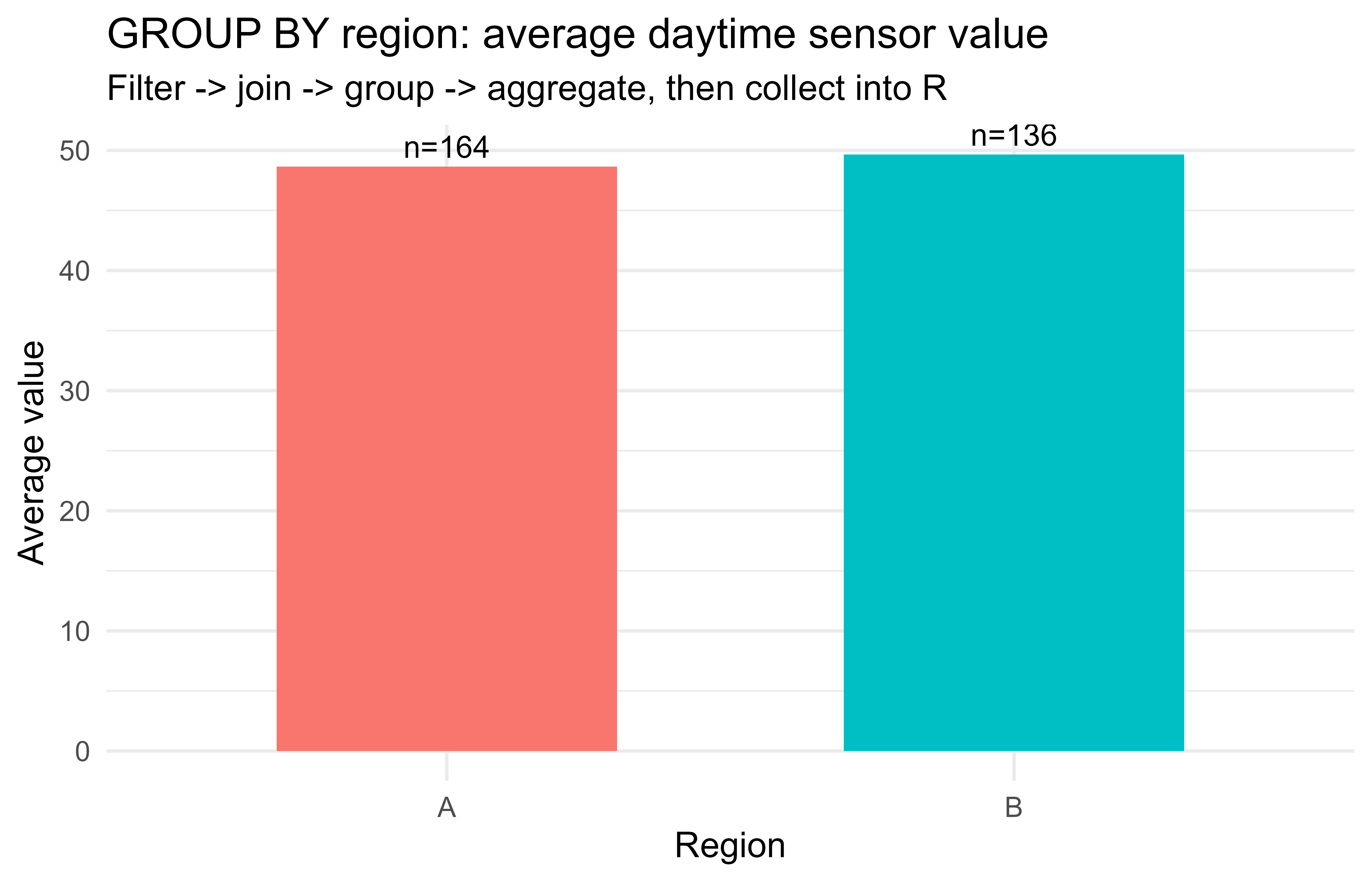
Figure 99.1: Average and count of measurements by group, computed with a relational-algebra pipeline over an in-memory base R ‘table’. This mirrors a GROUP BY query whose small result is collected into R for plotting.
Figure 99.1 shows the collected summary as a bar plot, with the per-group counts annotated above each bar. The demonstration deliberately mirrors a real dbplyr pipeline: a selection (WHERE), an equijoin (JOIN ... ON), a grouped aggregation (GROUP BY), and a final collect() that brings only the small summary into R for plotting. The parameter-binding helper shows why bound values are safe: the malicious string is compared as a literal and matches nothing, instead of being parsed as a second statement.
99.8 The same query three ways
To make the translation explicit, Table 99.2 expresses one analytical question in raw SQL, in dbplyr, and in the base R analogue above.
Table 99.2: The same filter, join, aggregate, materialize pipeline expressed three ways: raw SQL, dbplyr verbs, and the base R toy-engine analogue.
The point is that the three are the same relational-algebra program with three syntaxes. dbplyr exists so you can stay in dplyr and still get the database to do the heavy lifting. Once you can see a query through that lens, switching among the three is a matter of taste and tooling, not a new concept to learn each time.
99.9 Choosing a backend
The DBI interface is shared, but engines differ. Table 99.3 gives a short comparison of common choices.
Table 99.3: Common database engines reachable through DBI, their driver packages, typical uses, and distinguishing notes.
Engine
DBI driver
Typical use
Notes
SQLite
RSQLite
Local files, tests, embedded
Serverless, single file, great sandbox
DuckDB
duckdb
Local analytics on large files
Columnar, fast aggregations, reads Parquet/CSV directly
For analytical work on large local files, DuckDB has become a popular default because it is serverless like SQLite but columnar and fast for aggregations, and it queries Parquet and CSV files in place (the in-process analytics chapter, Chapter 100, covers this engine in depth).4 Because all of these engines share the DBI interface, switching among them costs almost nothing: the code differs only in the dbConnect() line.
When to use this
Use SQLite for tests and small embedded data, DuckDB for fast local analytics over big files, PostgreSQL or MySQL when the data lives in a shared production database, and the odbc driver when you must reach an enterprise warehouse such as Snowflake or SQL Server.
Show code
library(DBI)library(duckdb)con<-dbConnect(duckdb::duckdb())# in-process analytical engine# Query a Parquet file directly, no import step needed.dbGetQuery(con, "SELECT region, AVG(value) AS m FROM 'sensors.parquet' GROUP BY region")dbDisconnect(con, shutdown =TRUE)
99.10 Practical guidance, pitfalls, and when to use this
The concepts above turn into a handful of habits that separate smooth pipelines from slow or fragile ones. The following checklist collects the ones that matter most in day-to-day work:
Push work down, pull results up. Filter, join, and aggregate in the database; collect() only the reduced result. Inspect show_query() to confirm the work really is happening in SQL.
Collect late, not early. Calling collect() or as.data.frame() too soon drags the full table into R and defeats the purpose. Watch for accidental triggers: passing a lazy table to a function that calls nrow() or to a non-dbplyr function forces a pull.
Always parameterize. Use ? placeholders with params for values, and dbQuoteIdentifier() for dynamic table or column names. Never paste user input into SQL.
Close connections. Use on.exit(dbDisconnect(con)) or dbWithTransaction()/pool so connections do not leak, especially in loops, scheduled jobs, and Shiny apps (Chapter 114).
Mind translation gaps. Not every R function has a SQL equivalent in dbplyr. If translation errors, move that step after collect() or write the SQL by hand for that part.
Use transactions for multi-statement integrity and for bulk loads. Wrapping many inserts in one transaction is both safer and much faster than autocommitting each row.
Beware NULL versus NA and three-valued logic. In SQL, comparisons with NULL return unknown, not false, so WHERE x = NULL matches nothing; use IS NULL. dbplyr handles common cases, but check results when missingness matters.
Sampling and ordering can be expensive or nondeterministic. ORDER BY RANDOM() over a huge table is slow; prefer engine-specific sampling (TABLESAMPLE, DuckDB’s USING SAMPLE) for large draws.
Index the columns you filter and join on. A WHERE or JOIN on an unindexed column forces a full scan; this is often the difference between seconds and minutes.
Warning
The two mistakes that cause the most pain in practice are collecting too early (which silently drags the whole table into R) and pasting user input into SQL (which is both a bug and a security hole). If you internalize only two habits from this chapter, make them “collect late” and “always parameterize.”
When to use it: any time the data is larger than comfortable R memory, lives in a shared store, or must be joined across several source tables. For small data already in a flat file, plain readr/data.table plus dplyr is simpler and there is no reason to involve a database. The crossover point in practice is roughly when a single pull would strain memory or when the same join must be recomputed often enough that the database’s indexes and planner pay off.
99.11 Further reading
Codd (1970), “A Relational Model of Data for Large Shared Data Banks,” Communications of the ACM. The foundational paper on the relational model and relational algebra.
Wickham, Cetinkaya-Rundel, and Grolemund (2023), R for Data Science (2nd ed.), chapter on databases. Hands-on DBI and dbplyr usage, available free online.
Kuhn and Silge (2022), Tidy Modeling with R. Context for fitting models on data assembled from databases.
Date (2003), An Introduction to Database Systems. A thorough treatment of the relational model, SQL, and transactions.
Garcia-Molina, Ullman, and Widom (2008), Database Systems: The Complete Book. Query processing, optimization, and the algebra equivalences a planner uses.
The DBI, dbplyr, RSQLite, and duckdb package vignettes for current API details and engine-specific behavior.
Marking a chunk eval=FALSE only means the book does not execute it while compiling; it does not mean the code is untested or wrong. Copy any such chunk into an R session with the relevant package installed and it will run.↩︎
“Tuple” is just the database word for a row, and “attribute” the word for a column. A “domain” is the set of values a column is allowed to hold, for example the integers for an age column or a fixed set of strings for a status column.↩︎
A “generic” here is a function such as dbConnect() whose behavior is supplied by whichever driver package you loaded. This is the same idea as a plug standard: the wall socket is DBI, and each appliance is a backend that fits it.↩︎
A “columnar” engine stores each column together rather than each row together. Analytical queries that scan one or two columns of a wide table then read far less data, which is why DuckDB is fast for aggregations over large files.↩︎
Source Code
# Databases and SQL from R {#sec-databases-sql-r}```{r}#| include: falsesource("_common.R")``````{r dbsql-setup, include=FALSE}knitr::opts_chunk$set(echo =TRUE, message =FALSE, warning =FALSE)```Most real data does not live in a `.csv` file on your laptop. It lives in a database: a transactional store behind an application, a data warehouse, or an analytical engine that someone else maintains. A data scientist, analyst, or ML engineer who can only work with data after it has been exported to a flat file is limited to whatever someone else chose to export. The skill this chapter builds is the ability to pull exactly the rows and columns you need, computed where the data already sits, and bring only the result into R.The chapter covers the standard R interface to databases (`DBI`), how to write safe parameterized queries, and how `dbplyr` lets you write ordinary `dplyr` code that is translated into SQL and run inside the database. The mathematical content is the relational model and its algebra, which is what SQL is a syntax for. By the end you should be able to connect to a database from R, push filtering and aggregation into the engine, pull back only the small result you need, and recognize the safety and performance traps that bite people in production.::: {.callout-important title="Key idea"}The single most consequential choice in a data pipeline is *where* the computation happens. Doing the work in the database and shipping a small answer to R is usually faster, cheaper, and safer than shipping a huge table to R and working on it there.:::Because the database packages (`DBI`, `RSQLite`, `dbplyr`, `duckdb`) are outside the set of packages this book runs at build time, those chunks are marked `eval=FALSE`; they are correct, current code you can run.^[Marking a chunk `eval=FALSE` only means the book does not execute it while compiling; it does not mean the code is untested or wrong. Copy any such chunk into an R session with the relevant package installed and it will run.] A self-contained base R demonstration at the end teaches the same ideas with no external dependency, so you can see every concept run even without a database.## Where this fits in a modern ML and AI workflowA typical pipeline starts with raw data in a database and ends with a model or an analysis. The decision you make at the very first step, how much computation to push into the database versus pull into R, often dominates the runtime and the memory footprint of everything downstream.The principle is to do filtering, joining, and aggregation in the database, where the data already lives and where indexes and query planners exist, and to bring into R only the comparatively small, already-reduced table that you will model on. Pulling a billion-row table into R to then keep ten thousand rows is the most common and most expensive mistake.::: {.callout-tip title="Intuition"}Think of the database as a warehouse and R as your workbench. You do not haul the entire warehouse to your bench to find one box; you ask the warehouse to find the box and send it over. The "asking" is SQL, and the box is the result of your query.:::```[ database ] --SQL/dbplyr--> [ filtered, joined, aggregated result ] --collect()--> [ R data frame ] --> [ recipe / model / plot ]```This pattern appears everywhere in practice: assembling a feature table for a model by joining several source tables, computing label definitions with window functions, sampling a class-balanced training set with a stratified query, or scoring new records by reading them in batches. The same `DBI` connection object is also what monitoring code (@sec-model-monitoring), scheduled jobs, and feature stores (@sec-feature-stores) use.## The relational model and relational algebraBefore touching any package, it helps to know what SQL actually *is*. SQL is a concrete syntax for relational algebra, a small mathematical language for transforming tables. You do not need the algebra to write queries, but knowing it makes the translation that `dbplyr` performs predictable: once you can see a `dplyr` pipeline as a sequence of algebra operators, you can predict the SQL it will generate and reason about why one ordering of steps runs faster than another.A *relation* (the formal name for a table) is a set of tuples (rows) drawn from a Cartesian product of attribute domains (columns).^["Tuple" is just the database word for a row, and "attribute" the word for a column. A "domain" is the set of values a column is allowed to hold, for example the integers for an `age` column or a fixed set of strings for a `status` column.] Write a relation $R$ with attributes $A_1, \dots, A_k$ as a subset$$R \subseteq D_1 \times D_2 \times \cdots \times D_k,$$where $D_j$ is the domain (the set of allowed values) of attribute $A_j$. Each element of $R$ is one row.The core operators of relational algebra, and the SQL and `dplyr` verbs that express them, are:- Selection $\sigma_{\varphi}(R)$: keep the rows satisfying a predicate $\varphi$. In SQL this is `WHERE`; in `dplyr` it is `filter()`.$$\sigma_{\varphi}(R) = \{\, t \in R : \varphi(t) \text{ is true} \,\}.$$- Projection $\pi_{A_{i_1}, \dots, A_{i_m}}(R)$: keep a subset of columns. In SQL this is the `SELECT` list; in `dplyr` it is `select()`.- Cartesian product $R \times S$ and the *join* $R \bowtie_{\theta} S$, which is a product followed by a selection on a matching condition $\theta$:$$R \bowtie_{\theta} S = \sigma_{\theta}(R \times S).$$A common case is the equijoin where $\theta$ equates a key in $R$ with a key in $S$. In SQL this is `JOIN ... ON`; in `dplyr` it is `*_join()`.- Grouping and aggregation $\gamma_{G;\, f}(R)$: partition rows by the values of grouping attributes $G$ and apply an aggregate function $f$ (count, sum, mean) to each group. In SQL this is `GROUP BY`; in `dplyr` it is `group_by()` then `summarise()`.Two facts about this algebra matter for performance. First, the operators are *closed*: every operator takes relations and returns a relation, so they compose. Second, the algebra has *equivalences* that a query optimizer exploits, the most important being that selection can be pushed past a join,$$\sigma_{\varphi}(R \bowtie_{\theta} S) \equiv \sigma_{\varphi}(R) \bowtie_{\theta} S\quad\text{when } \varphi \text{ refers only to attributes of } R .$$Filtering before joining shrinks the inputs to the join. A SQL query planner applies such rewrites automatically; this is why pushing work into the database usually beats doing it in R after a naive full pull.::: {.callout-note}You will rarely write relational algebra by hand. Its value here is conceptual: every SQL query, and every `dbplyr` pipeline, is one of these algebra expressions in disguise. When a query is slow, the question to ask is almost always "did the engine get to filter before it joined?":::## DBI: the connection interfaceWith the algebra in mind, we can turn to the tools. The first is `DBI`, the database interface package. It defines a small, driver-independent set of generics, and each backend (`RSQLite`, `RPostgres`, `RMariaDB`, `duckdb`, `odbc`) implements them.^[A "generic" here is a function such as `dbConnect()` whose behavior is supplied by whichever driver package you loaded. This is the same idea as a plug standard: the wall socket is `DBI`, and each appliance is a backend that fits it.] Code written against `DBI` works across engines with little change, so you can prototype against SQLite on your laptop and later point the same code at PostgreSQL in production.Every database session follows the same three-step lifecycle: connect, query, disconnect. An in-memory SQLite database is the easiest sandbox because it needs no server and leaves nothing on disk.```{r dbsql-dbi-connect, eval=FALSE}library(DBI)library(RSQLite)# ":memory:" creates a private, in-memory database that vanishes on disconnect.con <-dbConnect(RSQLite::SQLite(), ":memory:")# Write an R data frame into the database as a table.dbWriteTable(con, "flights", nycflights13::flights)# List tables and inspect columns.dbListTables(con)dbListFields(con, "flights")# Run a query and pull the whole result into an R data frame.res <-dbGetQuery(con, "SELECT carrier, COUNT(*) AS n FROM flights GROUP BY carrier")head(res)# Always release the connection.dbDisconnect(con)```Out of the dozens of generics `DBI` defines, a handful carry almost all of the day-to-day work, sorted here by how often you reach for them:- `dbGetQuery(con, sql)`: run a `SELECT` and return the full result as a data frame. This is your workhorse for reading.- `dbExecute(con, sql)`: run a statement with no result set (`INSERT`, `UPDATE`, `CREATE`), returning the number of affected rows.- `dbSendQuery()` / `dbFetch()` / `dbClearResult()`: run a query and fetch the result in chunks, for results too large to hold in memory at once.- `dbWriteTable()` / `dbReadTable()`: move whole tables between R and the database.::: {.callout-tip}Reach for `dbGetQuery()` when the result is small enough to fit in memory, and for the `dbSendQuery()` / `dbFetch()` trio when it is not, so you can stream the result in batches rather than materializing it all at once.:::A connection is a live resource, like an open file handle, and leaking it can exhaust the database's connection limit. For long-running jobs, wrap the connection so it always closes, even when an error is thrown partway through:```{r dbsql-dbi-onexit, eval=FALSE}con <-dbConnect(RSQLite::SQLite(), ":memory:")on.exit(dbDisconnect(con), add =TRUE)# ... work with con ...```## Parameterized queries and SQL injection safetyKnowing how to run queries, the next thing to learn is how to run them *safely*. There is one rule that matters more than any other here: never build a SQL string by pasting user input into it. The reason is both correctness (quoting and escaping are error prone) and security (string concatenation is the mechanism behind SQL injection, a class of attack where the input is crafted to be read as SQL code instead of data). The classic illustration: suppose you concatenate a user-supplied name.::: {.callout-warning}If any part of your query string comes from outside your program (a web form, a file, an API call, a spreadsheet someone emailed you), treat it as hostile until it is bound as a parameter. The example below shows exactly how a friendly-looking input can become a `DROP TABLE`.:::```{r dbsql-injection, eval=FALSE}# DANGEROUS: do not do this.user_input <-"Smith'; DROP TABLE customers; --"bad_sql <-paste0("SELECT * FROM customers WHERE name = '", user_input, "'")bad_sql# SELECT * FROM customers WHERE name = 'Smith'; DROP TABLE customers; --'# The database sees two statements; the second deletes the table.```The fix is a *parameterized query* (also called a prepared statement): you write placeholders in the SQL and pass the values separately, so the driver sends the query structure and the data over different channels. The data can never be reinterpreted as SQL syntax. With `DBI` the placeholder is `?` and values go through the `params` argument.```{r dbsql-param, eval=FALSE}# SAFE: the value is bound as data, never parsed as SQL.safe <-dbGetQuery( con,"SELECT * FROM customers WHERE name = ?",params =list(user_input))# Multiple parameters bind positionally.dbGetQuery( con,"SELECT * FROM orders WHERE customer_id = ? AND amount > ?",params =list(42L, 100.0))```When you must build an *identifier* (a table or column name) dynamically, which cannot be a bound parameter, use `dbQuoteIdentifier()` rather than string pasting, and use `dbQuoteLiteral()` for literal values when a true parameter is not possible:```{r dbsql-quote, eval=FALSE}tbl <-dbQuoteIdentifier(con, "orders")sql <-paste0("SELECT COUNT(*) FROM ", tbl)dbGetQuery(con, sql)```The rule is simple, and worth committing to memory: values become parameters, identifiers get quoted with `dbQuoteIdentifier()`, and you never use `paste0()` to splice raw user input into SQL.::: {.callout-important title="Key idea"}A parameter is data on a separate wire from the query text. Because the driver never re-parses that wire as SQL, there is no string for an attacker to break out of. This is why parameterization fixes both the security problem and the quoting headaches at the same time.:::## dbplyr: dplyr translated to SQLWriting raw SQL by hand is fine, but if you already know `dplyr` there is a way to keep using it and still get the database to do the work. `dbplyr` is a `dplyr` backend for databases. You point `tbl()` at a database table, then write ordinary `dplyr` verbs. Instead of executing in R, the verbs are translated to SQL and executed in the database. You pull the result into R only when you call `collect()`.::: {.callout-tip title="When to use this"}Reach for `dbplyr` when you are comfortable in the tidyverse and your query is expressible with standard verbs (`filter`, `select`, joins, `group_by`/`summarise`). Drop to raw SQL through `DBI` when you need a feature `dbplyr` cannot translate, such as a database-specific function or a window expression it does not yet support.:::```{r dbsql-dbplyr, eval=FALSE}library(dplyr)library(dbplyr)flights_db <-tbl(con, "flights") # a lazy reference, not the dataquery <- flights_db %>%filter(month ==1, day ==1) %>%group_by(carrier) %>%summarise(avg_delay =mean(dep_delay, na.rm =TRUE), n =n()) %>%arrange(desc(avg_delay))# See the generated SQL without running it.show_query(query)# Now actually run it in the database and bring the small result to R.result <-collect(query)```The translation is mechanical and follows the algebra above: `filter()` becomes `WHERE`, `select()` becomes the `SELECT` list, `*_join()` becomes `JOIN`, and `group_by()` plus `summarise()` becomes `GROUP BY` with aggregate functions. R functions inside the verbs are mapped to their SQL equivalents where one exists (`mean` to `AVG`, `n()` to `COUNT(*)`, `toupper` to `UPPER`). Functions with no SQL equivalent will error at translation time, which is the signal to either compute that part after `collect()` or write raw SQL.### Lazy evaluation and collect()The central idea is *lazy evaluation*: the pipeline describes the work without doing it. A `dbplyr` pipeline builds up a query but does not run it. Nothing touches the database until you ask for results, either by printing (which fetches a small preview), by `collect()` (which runs the full query and returns a data frame), or by `compute()` (which materializes an intermediate result as a temporary table inside the database). This lets the whole pipeline be optimized and executed as one SQL statement rather than as a sequence of round trips.::: {.callout-tip title="Intuition"}A lazy query is like a recipe, not a cooked meal. You can add steps, rearrange them, and read the recipe (`show_query()`) for free. Only `collect()` turns on the stove, and only then does the database do real work.:::The comparison in @tbl-databases-sql-r-lazy-vs-eager contrasts the two ways of finishing a pipeline.| Aspect | Lazy `dbplyr` query | After `collect()`||---|---|---|| Where it runs | In the database engine | In R memory || When it runs | Only on `collect()`, `compute()`, or print | Immediately, eager R evaluation || Memory in R | Just the query definition | The full materialized result || Functions allowed | Those with a SQL translation | Any R function || Optimization | Database query planner | None beyond R itself || Right time to switch | After filtering, joining, aggregating | When the result is small and needs R-only work |: Lazy `dbplyr` query evaluation contrasted with eager R evaluation after `collect()`, across where and when the work runs, memory use, allowed functions, and optimization. {#tbl-databases-sql-r-lazy-vs-eager}The practical workflow: do as much as possible lazily so the data shrinks, inspect `show_query()` to confirm the SQL is sensible, then `collect()` the small result and continue with R-only tools (`ggplot2`, models, custom functions).## TransactionsReading data is only half the story; sometimes you change it, and changes that span several statements need to be all-or-nothing. A *transaction* groups several statements so they succeed or fail together. The guarantees are summarized by the acronym ACID: Atomicity (all statements commit or none do), Consistency (the database moves between valid states), Isolation (concurrent transactions do not see each other's partial work), and Durability (a committed result survives a crash). The canonical example is a transfer: debiting one account and crediting another must both happen or neither, because a crash in between would otherwise make money vanish.```{r dbsql-transaction, eval=FALSE}dbBegin(con)tryCatch( {dbExecute(con, "UPDATE accounts SET balance = balance - ? WHERE id = ?",params =list(100, 1L))dbExecute(con, "UPDATE accounts SET balance = balance + ? WHERE id = ?",params =list(100, 2L))dbCommit(con) },error =function(e) {dbRollback(con) # undo both updates if either failedstop(e) })````dbWithTransaction(con, { ... })` wraps this pattern: it commits if the block returns normally and rolls back if it throws, so you rarely need to call `dbBegin`/`dbCommit`/`dbRollback` by hand.::: {.callout-tip}Transactions are not only for safety, they are also a speed trick. Wrapping many inserts in one transaction is a large speedup, since each statement otherwise pays the cost of its own implicit commit (a disk sync) on every row.:::## A runnable demonstration in base REverything so far has been code you cannot run inside this book because the database packages are not installed at build time. To make the ideas concrete and executable, the following self-contained demonstration uses only base R and `ggplot2` to reproduce the same concepts: building a small relational table, running the relational-algebra operations that SQL performs, contrasting safe parameter binding with unsafe string pasting, and showing lazy versus eager evaluation. Think of the helper functions below as a paper-thin database engine. They are not how you would query a real database, but they make each SQL concept visible as a few lines of R you can read and run.::: {.callout-note}This section is a teaching model, not a recommendation. In real work you would use `DBI` and `dbplyr`, not hand-written `sel`/`proj`/`join_on` helpers. The point is to show that "filter, join, group, collect" is the same program whether it runs in SQLite, in PostgreSQL, or in the toy engine below.:::```{r fig-databases-sql-r-group-by-region, eval=TRUE, fig.width=7, fig.height=4.5, fig.cap="Average and count of measurements by group, computed with a relational-algebra pipeline over an in-memory base R 'table'. This mirrors a GROUP BY query whose small result is collected into R for plotting."}.libPaths(c("C:/Users/miken/R/library-4.4", .libPaths()))suppressPackageStartupMessages(library(ggplot2))set.seed(1)# 1. Create an in-memory "table": a data frame is a relation (a set of rows).n <-600sensors <-data.frame(id =seq_len(n),site =sample(c("north", "south", "east", "west"), n, replace =TRUE),hour =sample(0:23, n, replace =TRUE),value =round(rnorm(n, mean =50, sd =10), 2),stringsAsFactors =FALSE)# A lookup table to demonstrate a join (an equijoin on the key "site").site_info <-data.frame(site =c("north", "south", "east", "west"),region =c("A", "A", "B", "B"),stringsAsFactors =FALSE)# 2. Relational-algebra operators implemented in base R.# selection sigma_phi : keep rows satisfying a predicatesel <-function(df, keep) df[keep, , drop =FALSE]# projection pi : keep a subset of columnsproj <-function(df, cols) df[, cols, drop =FALSE]# equijoin R |><| S on a shared keyjoin_on <-function(R, S, key) merge(R, S, by = key)# grouping + aggregation gammaagg <-function(df, by, fun) { out <-aggregate(df["value"], by = df[by], FUN = fun) out}# 3. A query: daytime readings (hour 6..18), joined to region,# then average value and count per region.# selection: WHERE hour BETWEEN 6 AND 18day <-sel(sensors, sensors$hour >=6& sensors$hour <=18)# join: JOIN site_info ON siteday <-join_on(day, site_info, "site")# group + aggregate: GROUP BY regionmeans <-agg(day, "region", function(v) mean(v))counts <-agg(day, "region", function(v) length(v))summary_tbl <-data.frame(region = means$region,avg_value =round(means$value, 2),n = counts$value)print(summary_tbl)# 4. Parameterized-query safety, illustrated without a real database.# A "binding" function treats the value strictly as data:run_param <-function(df, column, value) {# value is compared as data; it is never interpreted as code/SQL. df[df[[column]] == value, , drop =FALSE]}malicious <-"north'; DROP TABLE sensors; --"# would be dangerous if pastedsafe_rows <-run_param(sensors, "site", malicious)cat("Rows returned for the malicious 'site' value:", nrow(safe_rows), "\n")cat("The injected text was treated as a literal value, so it matched nothing.\n")# 5. Lazy vs eager evaluation. Build a query as an unevaluated promise,# then "collect()" it to force execution, mirroring dbplyr.lazy_query <-function(expr) { q <-substitute(expr) # capture, do not runstructure(list(call = q, env =parent.frame()), class ="lazy_query")}collect_q <-function(q) eval(q$call, q$env) # force execution nowq <-lazy_query(aggregate(value ~ site, data = sensors[sensors$hour >=6, ], FUN = mean))cat("Built a lazy query object; nothing has executed yet.\n")by_site <-collect_q(q) # execution happens here, like collect()by_site$value <-round(by_site$value, 2)# 6. Figure produced from the collected (small) result.ggplot(summary_tbl, aes(x = region, y = avg_value, fill = region)) +geom_col(width =0.6) +geom_text(aes(label =paste0("n=", n)), vjust =-0.4, size =4) +labs(title ="GROUP BY region: average daytime sensor value",subtitle ="Filter -> join -> group -> aggregate, then collect into R",x ="Region", y ="Average value" ) +theme_minimal(base_size =13) +theme(legend.position ="none")```@fig-databases-sql-r-group-by-region shows the collected summary as a bar plot, with the per-group counts annotated above each bar. The demonstration deliberately mirrors a real `dbplyr` pipeline: a selection (`WHERE`), an equijoin (`JOIN ... ON`), a grouped aggregation (`GROUP BY`), and a final `collect()` that brings only the small summary into R for plotting. The parameter-binding helper shows why bound values are safe: the malicious string is compared as a literal and matches nothing, instead of being parsed as a second statement.## The same query three waysTo make the translation explicit, @tbl-databases-sql-r-three-ways expresses one analytical question in raw SQL, in `dbplyr`, and in the base R analogue above.| Step | SQL | dbplyr | base R analogue ||---|---|---|---|| Source |`FROM sensors`|`tbl(con, "sensors")`|`sensors` data frame || Filter |`WHERE hour BETWEEN 6 AND 18`|`filter(hour >= 6, hour <= 18)`|`sel(sensors, ...)`|| Join |`JOIN site_info USING (site)`|`inner_join(site_info, by = "site")`|`join_on(., site_info, "site")`|| Aggregate |`GROUP BY region` with `AVG`, `COUNT`|`group_by(region) %>% summarise(...)`|`agg(., "region", mean)`|| Materialize | run the statement |`collect()`|`collect_q()`|: The same filter, join, aggregate, materialize pipeline expressed three ways: raw SQL, `dbplyr` verbs, and the base R toy-engine analogue. {#tbl-databases-sql-r-three-ways}The point is that the three are the same relational-algebra program with three syntaxes. `dbplyr` exists so you can stay in `dplyr` and still get the database to do the heavy lifting. Once you can see a query through that lens, switching among the three is a matter of taste and tooling, not a new concept to learn each time.## Choosing a backendThe `DBI` interface is shared, but engines differ. @tbl-databases-sql-r-backends gives a short comparison of common choices.| Engine | DBI driver | Typical use | Notes ||---|---|---|---|| SQLite |`RSQLite`| Local files, tests, embedded | Serverless, single file, great sandbox || DuckDB |`duckdb`| Local analytics on large files | Columnar, fast aggregations, reads Parquet/CSV directly || PostgreSQL |`RPostgres`| Production OLTP and warehouses | Rich SQL, strong concurrency || MySQL/MariaDB |`RMariaDB`| Application databases | Widespread, web stack default || Any ODBC source |`odbc`| Enterprise warehouses (Snowflake, SQL Server, Redshift) | One driver, many backends |: Common database engines reachable through `DBI`, their driver packages, typical uses, and distinguishing notes. {#tbl-databases-sql-r-backends}For analytical work on large local files, DuckDB has become a popular default because it is serverless like SQLite but columnar and fast for aggregations, and it queries Parquet and CSV files in place (the in-process analytics chapter, @sec-duckdb-arrow, covers this engine in depth).^[A "columnar" engine stores each column together rather than each row together. Analytical queries that scan one or two columns of a wide table then read far less data, which is why DuckDB is fast for aggregations over large files.] Because all of these engines share the `DBI` interface, switching among them costs almost nothing: the code differs only in the `dbConnect()` line.::: {.callout-tip title="When to use this"}Use SQLite for tests and small embedded data, DuckDB for fast local analytics over big files, PostgreSQL or MySQL when the data lives in a shared production database, and the `odbc` driver when you must reach an enterprise warehouse such as Snowflake or SQL Server.:::```{r dbsql-duckdb, eval=FALSE}library(DBI)library(duckdb)con <-dbConnect(duckdb::duckdb()) # in-process analytical engine# Query a Parquet file directly, no import step needed.dbGetQuery(con, "SELECT region, AVG(value) AS m FROM 'sensors.parquet' GROUP BY region")dbDisconnect(con, shutdown =TRUE)```## Practical guidance, pitfalls, and when to use thisThe concepts above turn into a handful of habits that separate smooth pipelines from slow or fragile ones. The following checklist collects the ones that matter most in day-to-day work:- Push work down, pull results up. Filter, join, and aggregate in the database; `collect()` only the reduced result. Inspect `show_query()` to confirm the work really is happening in SQL.- Collect late, not early. Calling `collect()` or `as.data.frame()` too soon drags the full table into R and defeats the purpose. Watch for accidental triggers: passing a lazy table to a function that calls `nrow()` or to a non-`dbplyr` function forces a pull.- Always parameterize. Use `?` placeholders with `params` for values, and `dbQuoteIdentifier()` for dynamic table or column names. Never paste user input into SQL.- Close connections. Use `on.exit(dbDisconnect(con))` or `dbWithTransaction()`/`pool` so connections do not leak, especially in loops, scheduled jobs, and Shiny apps (@sec-ai-apps-shiny).- Mind translation gaps. Not every R function has a SQL equivalent in `dbplyr`. If translation errors, move that step after `collect()` or write the SQL by hand for that part.- Use transactions for multi-statement integrity and for bulk loads. Wrapping many inserts in one transaction is both safer and much faster than autocommitting each row.- Beware `NULL` versus `NA` and three-valued logic. In SQL, comparisons with `NULL` return unknown, not false, so `WHERE x = NULL` matches nothing; use `IS NULL`. `dbplyr` handles common cases, but check results when missingness matters.- Sampling and ordering can be expensive or nondeterministic. `ORDER BY RANDOM()` over a huge table is slow; prefer engine-specific sampling (`TABLESAMPLE`, DuckDB's `USING SAMPLE`) for large draws.- Index the columns you filter and join on. A `WHERE` or `JOIN` on an unindexed column forces a full scan; this is often the difference between seconds and minutes.::: {.callout-warning}The two mistakes that cause the most pain in practice are collecting too early (which silently drags the whole table into R) and pasting user input into SQL (which is both a bug and a security hole). If you internalize only two habits from this chapter, make them "collect late" and "always parameterize.":::When to use it: any time the data is larger than comfortable R memory, lives in a shared store, or must be joined across several source tables. For small data already in a flat file, plain `readr`/`data.table` plus `dplyr` is simpler and there is no reason to involve a database. The crossover point in practice is roughly when a single pull would strain memory or when the same join must be recomputed often enough that the database's indexes and planner pay off.## Further reading- Codd (1970), "A Relational Model of Data for Large Shared Data Banks," *Communications of the ACM*. The foundational paper on the relational model and relational algebra.- Wickham, Cetinkaya-Rundel, and Grolemund (2023), *R for Data Science* (2nd ed.), chapter on databases. Hands-on `DBI` and `dbplyr` usage, available free online.- Kuhn and Silge (2022), *Tidy Modeling with R*. Context for fitting models on data assembled from databases.- Date (2003), *An Introduction to Database Systems*. A thorough treatment of the relational model, SQL, and transactions.- Garcia-Molina, Ullman, and Widom (2008), *Database Systems: The Complete Book*. Query processing, optimization, and the algebra equivalences a planner uses.- The `DBI`, `dbplyr`, `RSQLite`, and `duckdb` package vignettes for current API details and engine-specific behavior.