47  Double Descent

The double descent phenomenon is an intriguing empirical observation in the context of machine learning. To understand it, let’s first consider the traditional U-shaped bias-variance trade-off curve:

1. As model complexity (such as the number of parameters) increases, the training error typically decreases.

2. The test error initially decreases, reaches a minimum, then increases due to overfitting, forming a U-shaped curve.

However, recent empirical studies have shown that as the model complexity continues to increase well beyond the interpolation threshold (where the model perfectly fits the training data), the test error surprisingly starts to decrease again. This results in a double descent curve: the test error first descends, ascends, and then descends again.

“Deep double descent” specifically refers to this phenomenon observed in deep learning models (see Chapter 15) (Nakkiran, Kaplun, et al. 2021).

47.1 Formulation

To make the phenomenon precise we fix notation. Let the data be \(n\) i.i.d. pairs \((x_i, y_i)\), \(i = 1, \dots, n\), with \(x_i \in \mathbb{R}^d\) and \(y_i \in \mathbb{R}\), drawn from a joint law \(P\). We consider a parametric family of predictors \(f_\theta\) indexed by \(\theta \in \mathbb{R}^p\), and define the population (test) risk and the empirical (training) risk under squared loss as \[ R(\theta) = \mathbb{E}_{(x,y)\sim P}\!\left[(y - f_\theta(x))^2\right], \qquad \hat R_n(\theta) = \frac{1}{n}\sum_{i=1}^n (y_i - f_\theta(x_i))^2 . \tag{47.1}\]

The key control variable is the parameterization ratio \[ \gamma = \frac{p}{n}, \tag{47.2}\] the number of free parameters \(p\) relative to the number of training points \(n\). The interpolation threshold is the smallest model complexity at which the training loss can be driven to zero, i.e. \(\hat R_n(\hat\theta) = 0\). For a linear model in \(p\) features fit by least squares this occurs at \(p = n\), that is \(\gamma = 1\), where the design matrix becomes square. The classical bias-variance regime is \(\gamma < 1\) (underparameterized); the modern regime is \(\gamma > 1\) (overparameterized), where infinitely many parameter vectors interpolate the data and a selection rule (an inductive bias) is needed to pick one.

The double descent curve is the graph of the test risk \(R(\hat\theta)\) as a function of \(\gamma\) (or of \(p\) with \(n\) fixed). It exhibits the classical U on \(\gamma < 1\), a spike that diverges as \(\gamma \to 1\), and a second descent for \(\gamma > 1\).

Note

The horizontal axis can be model size \(p\) (model-wise double descent), training-set size \(n\) (sample-wise non-monotonicity, where more data can temporarily hurt), or training time / epochs (epoch-wise double descent). All three are governed by the same effective ratio \(\gamma = p/n\) once a notion of “effective parameters” is defined (Nakkiran, Kaplun, et al. 2021).

47.2 The minimum-norm interpolator and its inductive bias

The behavior for \(\gamma > 1\) is not magic: it is a property of which interpolating solution the algorithm selects. For least squares with design matrix \(X \in \mathbb{R}^{n\times p}\) and response \(y \in \mathbb{R}^n\), the estimator is \[ \hat\beta = \arg\min_{\beta}\; \lVert y - X\beta\rVert_2^2 . \tag{47.3}\]

When \(p > n\) and \(\mathrm{rank}(X) = n\), this problem is underdetermined: the set of minimizers is an affine subspace \(\{\beta : X\beta = y\}\) of dimension \(p - n\). Gradient descent started at \(\beta = 0\), the Moore-Penrose pseudoinverse, and ridge regression in the limit of vanishing penalty all converge to the unique minimum-\(\ell_2\)-norm interpolator \[ \hat\beta = \arg\min_{\beta}\; \lVert\beta\rVert_2^2 \quad\text{s.t.}\quad X\beta = y, \qquad \hat\beta = X^\top (XX^\top)^{-1} y = X^+ y, \tag{47.4}\] where \(X^+\) is the pseudoinverse. We derive Equation 47.4 by Lagrangian duality. Form \[ \mathcal{L}(\beta, \lambda) = \tfrac12\lVert\beta\rVert_2^2 + \lambda^\top (y - X\beta), \qquad \nabla_\beta \mathcal{L} = \beta - X^\top\lambda = 0 \;\Rightarrow\; \beta = X^\top\lambda . \] Substituting the constraint \(X\beta = y\) gives \(XX^\top \lambda = y\), hence \(\lambda = (XX^\top)^{-1}y\) (using \(\mathrm{rank}(X)=n\)), and \(\hat\beta = X^\top(XX^\top)^{-1}y\). That gradient descent on Equation 47.3 from \(\beta=0\) lands exactly here follows because every gradient step \(\beta \leftarrow \beta - \eta X^\top(X\beta - y)\) keeps the iterate inside the row space of \(X\), and within that subspace there is a unique interpolator, namely the minimum-norm one. The second descent is therefore a statement about the implicit regularization of the optimizer: as \(p\) grows past \(n\), the constraint set \(\{X\beta = y\}\) grows, the minimum-norm solution in that larger set has smaller norm, and the effective complexity of the selected function decreases even as the nominal parameter count increases.

47.3 Why the test error spikes at the interpolation threshold

The divergence at \(\gamma = 1\) has a clean algebraic cause: ill-conditioning. The risk of the minimum-norm interpolator depends on \((XX^\top)^{-1}\) (for \(\gamma > 1\)) or \((X^\top X)^{-1}\) (for \(\gamma < 1\)). As \(\gamma \to 1\), the relevant Gram matrix becomes nearly square and its smallest singular value \(\sigma_{\min}\) approaches zero. Writing the singular value decomposition \(X = U \Sigma V^\top\) with singular values \(\sigma_1 \ge \cdots \ge \sigma_{\min} > 0\), the noise component of the estimator inflates as \[ \mathbb{E}\big[\lVert \hat\beta - \beta^\star \rVert_2^2 \mid X\big] \;\geq\; \sigma^2 \sum_{j} \frac{1}{\sigma_j^2}, \tag{47.5}\] so a single vanishing \(\sigma_j\) drives the variance, and hence the test risk, to infinity. This is the variance explosion that produces the peak. The two descents flank the peak because in both directions away from \(\gamma = 1\) the spectrum of \(X\) moves away from singularity: for \(\gamma \ll 1\) there are few parameters to estimate (low variance, high bias), and for \(\gamma \gg 1\) the minimum-norm bias shrinks the solution and the bulk of the spectrum is again well separated from zero.

47.3.1 Bias-variance under the new lens

The classical decomposition still holds pointwise, \[ \mathbb{E}\big[(y_0 - f_{\hat\theta}(x_0))^2\big] = \underbrace{\sigma^2}_{\text{irreducible}} + \underbrace{\big(\mathbb{E}[f_{\hat\theta}(x_0)] - f^\star(x_0)\big)^2}_{\text{bias}^2} + \underbrace{\mathrm{Var}\big(f_{\hat\theta}(x_0)\big)}_{\text{variance}}, \tag{47.6}\] but the variance is no longer monotone in \(p\). It rises through the underparameterized regime, peaks at \(\gamma = 1\), and then falls in the overparameterized regime because the minimum-norm constraint caps the magnitude of \(\hat\beta\). The bias, meanwhile, keeps decreasing with \(p\) as the hypothesis class enriches. The sum of a peaked variance and a decreasing bias is exactly the double-descent shape. Double descent is thus fully consistent with the bias-variance trade-off; what fails is the naive identification of “variance” with “raw parameter count”.

47.4 Random-features asymptotics

The phenomenon admits an exact analysis in the proportional asymptotic regime \(n, p \to \infty\) with \(\gamma = p/n\) fixed, using random matrix theory (the Marchenko-Pastur law for the spectrum of \(\tfrac1n X^\top X\)). For an isotropic linear model \(y = X\beta^\star + \varepsilon\) with \(\mathrm{Var}(\varepsilon) = \sigma^2\) and \(\lVert\beta^\star\rVert_2^2 = r^2\), the asymptotic test risk of the minimum-norm least squares estimator is, up to model-specific constants (Hastie et al. 2022; Belkin et al. 2019), \[ R(\gamma) \;\to\; \begin{cases} \sigma^2\,\dfrac{\gamma}{1-\gamma}, & \gamma < 1,\\[2.2ex] r^2\Big(1 - \dfrac{1}{\gamma}\Big) + \sigma^2\,\dfrac{1}{\gamma - 1}, & \gamma > 1. \end{cases} \tag{47.7}\] Both branches diverge as \(\gamma \to 1^{\mp}\) (the variance term \(\sigma^2\,\gamma/(1-\gamma)\) for \(\gamma < 1\) and \(\sigma^2/(\gamma-1)\) for \(\gamma > 1\), both of which blow up like \(\sigma^2/|1-\gamma|\) as \(\gamma \to 1\)), confirming the spike. For \(\gamma > 1\) the first term is the bias from the unfittable \(p - n\) directions and decreases in \(\gamma\), while the variance term \(\sigma^2/(\gamma-1)\) also decreases, so the curve descends a second time and approaches the null risk \(r^2\) as \(\gamma \to \infty\). This closed form makes three points rigorous: (i) the peak is purely a variance effect tied to \(1/|1-\gamma|\); (ii) the second descent requires signal, \(r^2 < \infty\), and shrinking noise sensitivity; (iii) the global minimum can lie in either regime depending on the signal-to-noise ratio \(r^2/\sigma^2\).

Warning

Equation Equation 47.7 is for the un-regularized minimum-norm estimator. With optimal ridge regularization the peak is entirely removed: the test risk becomes a monotone, single-valued function of \(\gamma\) (Nakkiran, Venkat, et al. 2021). Double descent is therefore a symptom of missing (or implicit-only) regularization, not an intrinsic obstacle.

47.5 Connections, variants, and failure modes

• Optimal regularization erases it. Cross-validated ridge or weight decay tuned per \(\gamma\) yields a monotone risk curve. The classical advice “regularize, then increase capacity” remains correct.
• Effective parameters, not raw count. For kernels, random features, and deep nets the relevant \(\gamma\) uses an effective dimension (e.g. the number of features that survive, or the trace of the smoother matrix), which is why the peak in deep nets appears at a capacity well below the literal parameter count.
• Ensembling and bagging average out the high-variance interpolators near \(\gamma = 1\), flattening the peak, which connects double descent to the variance-reduction theory of random forests (Chapter 10).
• Failure modes. The second descent need not reach a useful minimum: if the signal-to-noise ratio is low, the overparameterized plateau in Equation 47.7 sits at \(r^2\), which may exceed the best underparameterized risk. Interpolating pure label noise (the “noiseless second descent”) only helps when an implicit norm bias is present; a different optimizer with a different implicit bias can produce a worse interpolator.

47.6 How to observe and manage it in practice

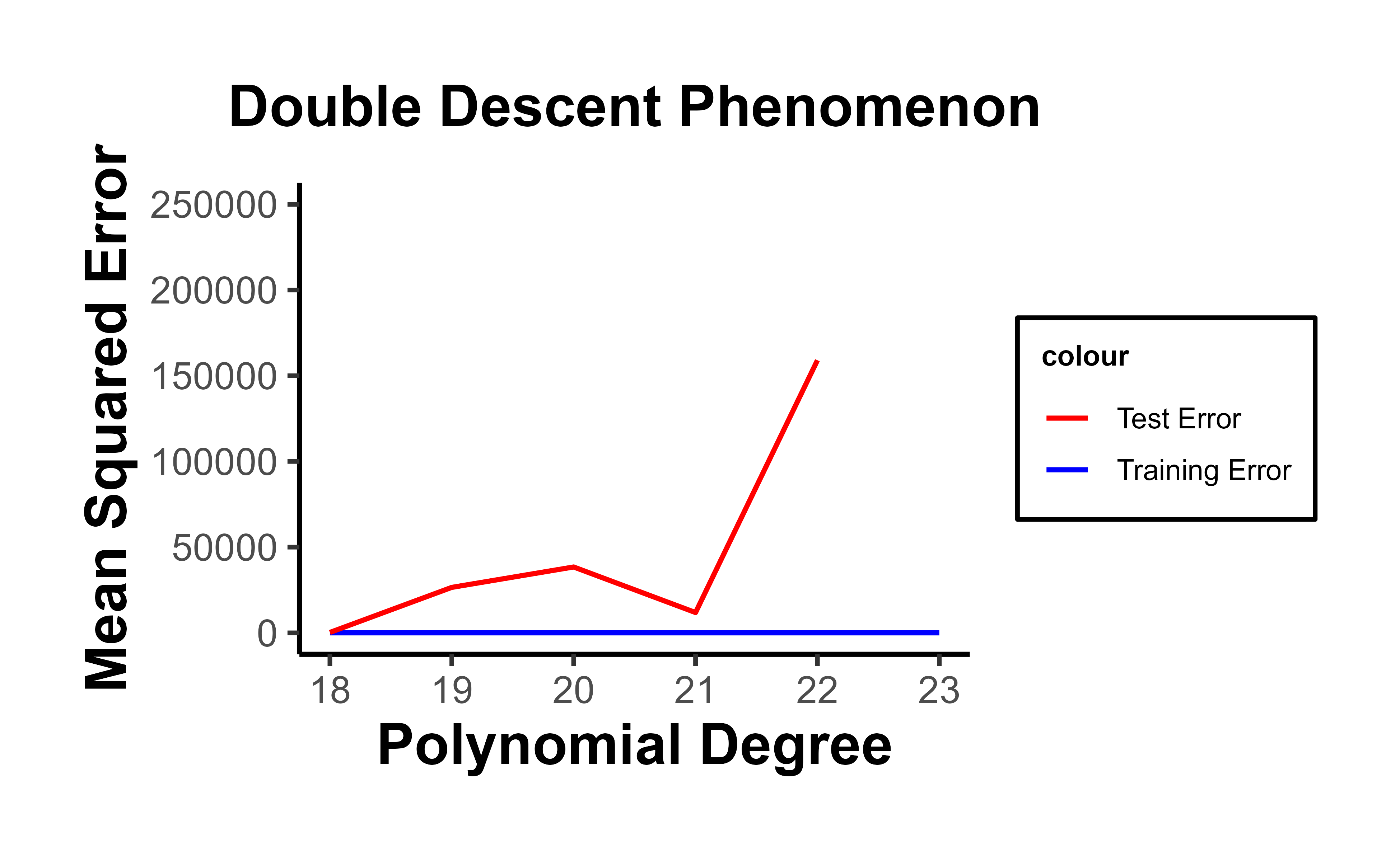
1. Sweep capacity finely near \(\gamma = 1\). The peak is narrow; a coarse grid of model sizes can step over it and hide the phenomenon entirely. The toy sweep below restricts the polynomial degree to the neighborhood of \(n/2\) training points precisely for this reason.
2. Watch the condition number. Plotting \(\sigma_{\min}(X)\) or the condition number \(\kappa(X)\) alongside test error makes the mechanism in Equation 47.5 visible: the error spike coincides with \(\kappa \to \infty\).
3. If you only care about generalization, regularize. A small ridge penalty \(\lambda\) both conditions the linear system and removes the peak; tune \(\lambda\) by cross-validation rather than chasing the second descent.
4. If you must interpolate (large nets), go well past the threshold. Operating at \(\gamma \gg 1\) with an implicit norm bias is safer than sitting at \(\gamma \approx 1\), where variance is maximal.

Tip

The numerical instability near \(\gamma = 1\) means raw poly(..., raw = TRUE) design matrices are severely ill-conditioned at high degree. The spike you see in the figure is partly genuine variance explosion and partly floating-point error from inverting a near-singular Vandermonde matrix; orthogonal polynomials (raw = FALSE) or an explicit ridge penalty give a numerically cleaner picture of the same statistical effect.

library(ggplot2)
library(MASS)

# Generate toy data
set.seed(123)
n <- 100
x <- seq(-pi, pi, length.out = n)
y <- sin(x) + rnorm(n, 0, 0.5)

# Split data into training and test sets
train_indices <- sample(1:n, n/2)
x_train <- x[train_indices]
y_train <- y[train_indices]
x_test <- x[-train_indices]
y_test <- y[-train_indices]

# Calculate training and test errors for polynomial regressions of different degrees
max_degree <- 25
train_errors <- numeric(max_degree)
test_errors <- numeric(max_degree)

for (degree in 1:max_degree) {
  model <- lm(y_train ~ poly(x_train, degree, raw=TRUE))
  y_train_pred <- predict(model, data.frame(x_train=x_train))
  y_test_pred <- predict(model, data.frame(x_train=x_test))
  
  train_errors[degree] <- mean((y_train_pred - y_train)^2)
  test_errors[degree] <- mean((y_test_pred - y_test)^2)
}

# Plot the errors
df <- data.frame(
    Degree = 1:max_degree,
    Training_Error = train_errors,
    Test_Error = test_errors
)

ggplot(df, aes(x = Degree)) +
    geom_line(aes(y = Training_Error, color = "Training Error")) +
    geom_line(aes(y = Test_Error, color = "Test Error")) +
    labs(title = "Double Descent Phenomenon", y = "Mean Squared Error", x =
             "Polynomial Degree") +
    scale_color_manual(values = c("Training Error" = "blue", "Test Error" =
                                      "red")) +
    causalverse::ama_theme() +
    xlim(18, 23) +
    ylim(0, 250000)

47.6.1 Regularization removes the peak

The spike at the interpolation threshold is not inevitable — it is specific to the minimum-norm interpolator that ordinary least squares falls back on when \(p > n\). The practical remedy is the oldest one in the book: a ridge penalty. Hold \(n = 100\) fixed, sweep the number of features \(p\) straight through the threshold, and compare the unregularized excess risk against ridge:

set.seed(1)
n <- 100                                              # interpolation threshold at p = n
fit <- function(X, y, lambda) {
  p <- ncol(X)
  if (lambda > 0)  solve(crossprod(X) + lambda * diag(p), crossprod(X, y))
  else if (p <= n) solve(crossprod(X), crossprod(X, y))
  else             crossprod(X, solve(tcrossprod(X), y))   # minimum-norm interpolator
}
risk <- function(p, lambda, reps = 40) mean(replicate(reps, {
  beta <- rnorm(p, sd = 1 / sqrt(p))
  X <- matrix(rnorm(n * p), n, p); y <- X %*% beta + rnorm(n, 0, 1)
  sum((beta - fit(X, y, lambda))^2)                   # excess risk, test features ~ N(0, I)
}))
ps <- c(20, 50, 80, 95, 105, 140, 200, 400)
rbind(p          = ps,
      min_norm   = round(sapply(ps, risk, lambda = 0), 2),
      ridge      = round(sapply(ps, risk, lambda = 5), 2))
#>           [,1]  [,2]  [,3]  [,4]   [,5]   [,6]   [,7]   [,8]
#> p        20.00 50.00 80.00 95.00 105.00 140.00 200.00 400.00
#> min_norm  0.25  0.99  4.58 18.66  20.91   2.90   1.48   1.09
#> ridge     0.22  0.72  1.45  1.88   1.99   1.77   1.34   1.05

The min_norm row traces the full double descent: risk climbs to a sharp peak as \(p\) approaches \(n = 100\) (the model is forced to interpolate noise with a wildly large-norm solution), then descends a second time as extra features give the minimum-norm solution room to stay small. The ridge row barely moves — a modest penalty caps the solution norm exactly where it would otherwise explode, cutting the peak by an order of magnitude and restoring an ordinary, monotone-looking risk curve. This is the operational lesson behind the phenomenon: double descent is mostly a story about implicit regularization being weak near the threshold, and a touch of explicit regularization, tuned by cross-validation as usual, makes the whole spike disappear. You rarely have to live on the peak.

47.6.2 Verifying the asymptotic risk formula

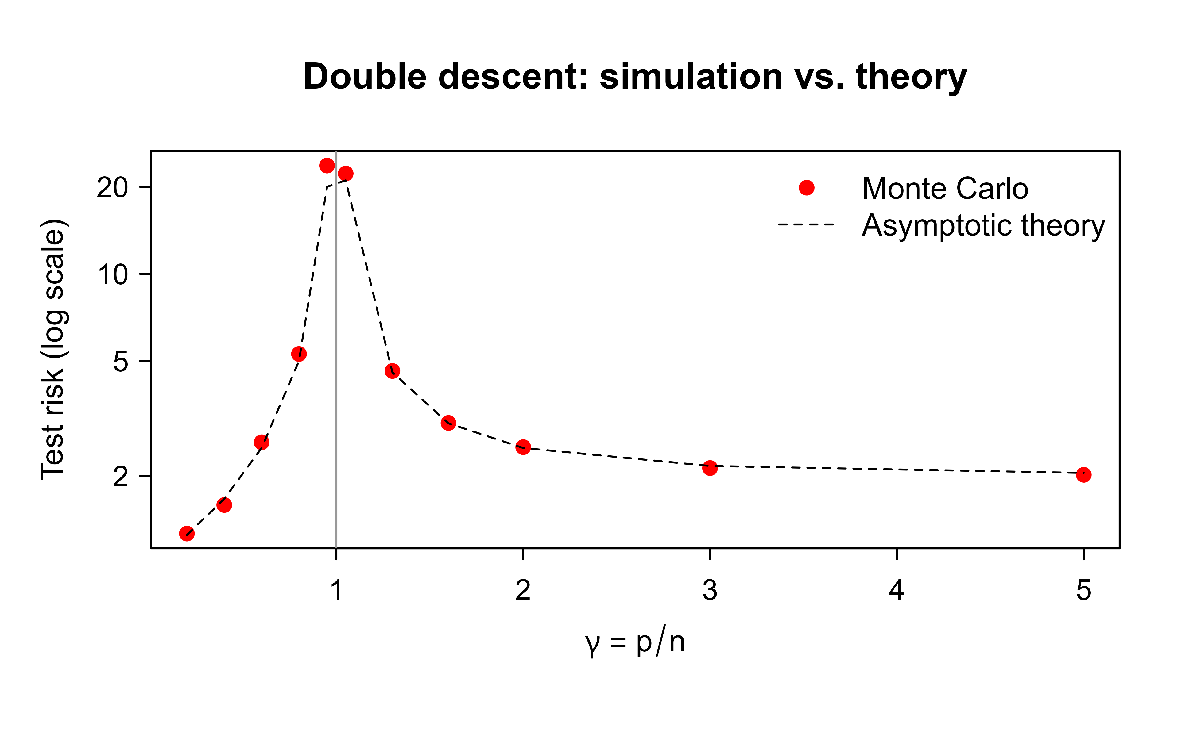
The following base-R simulation confirms Equation 47.7 for the isotropic linear model. We fix \(n\), vary \(p\), fit the minimum-norm least squares solution via the pseudoinverse (MASS::ginv), and compare the Monte Carlo test risk to the theory. The empirical curve tracks the closed form and blows up at \(\gamma = 1\).

set.seed(1)
n      <- 200          # training size
sigma2 <- 1            # noise variance
r2     <- 1            # signal energy ||beta*||^2 = sum(beta*^2)
ps     <- round(n * c(.2,.4,.6,.8,.95,1.05,1.3,1.6,2,3,5))
reps   <- 40

risk_emp <- sapply(ps, function(p) {
  beta_star <- rnorm(p, sd = sqrt(r2 / p))   # ||beta*||^2 ~ r2
  err <- replicate(reps, {
    X  <- matrix(rnorm(n * p), n, p)
    y  <- X %*% beta_star + rnorm(n, sd = sqrt(sigma2))
    bh <- MASS::ginv(X) %*% y                 # minimum-norm interpolator
    Xt <- matrix(rnorm(n * p), n, p)          # fresh test design
    yt <- Xt %*% beta_star + rnorm(n, sd = sqrt(sigma2))
    mean((yt - Xt %*% bh)^2)
  })
  mean(err)
})

gamma <- ps / n
risk_theory <- ifelse(
  gamma < 1,
  sigma2 * gamma / (1 - gamma) + sigma2,                 # + irreducible noise
  r2 * (1 - 1 / gamma) + sigma2 / (gamma - 1) + sigma2
)

plot(gamma, risk_emp, log = "y", pch = 19, col = "red",
     xlab = expression(gamma == p / n), ylab = "Test risk (log scale)",
     main = "Double descent: simulation vs. theory")
lines(sort(gamma), risk_theory[order(gamma)], lty = 2)
abline(v = 1, col = "grey60")
legend("topright", c("Monte Carlo", "Asymptotic theory"),
       pch = c(19, NA), lty = c(NA, 2), col = c("red", "black"), bty = "n")

Figure 47.1: Minimum-norm least squares test risk versus the parameterization ratio gamma. Points are Monte Carlo estimates; the dashed line is the asymptotic theory of equation (eq-double-descent.qmd-asymptotic-risk).

Belkin, Mikhail, Daniel Hsu, Siyuan Ma, and Soumik Mandal. 2019. “Reconciling Modern Machine-Learning Practice and the Classical Bias-Variance Trade-Off.” Proceedings of the National Academy of Sciences 116 (32): 15849–54.

Hastie, Trevor, Andrea Montanari, Saharon Rosset, and Ryan J. Tibshirani. 2022. “Surprises in High-Dimensional Ridgeless Least Squares Interpolation.” The Annals of Statistics 50 (2): 949–86.

Nakkiran, Preetum, Gal Kaplun, Yamini Bansal, Tristan Yang, Boaz Barak, and Ilya Sutskever. 2021. “Deep Double Descent: Where Bigger Models and More Data Hurt.” Journal of Statistical Mechanics: Theory and Experiment 2021 (12): 124003.

Nakkiran, Preetum, Prayaag Venkat, Sham Kakade, and Tengyu Ma. 2021. “Optimal Regularization Can Mitigate Double Descent.” In International Conference on Learning Representations (ICLR).