63  Metric and Similarity Learning

Two photographs of the same person, taken years apart under different lighting, should count as “close.” Two photographs of different people, even with similar haircuts and backgrounds, should count as “far.” A plain pixel-by-pixel distance gets this backwards almost every time: it is dominated by lighting, pose, and background, the very things we want to ignore. The problem is not the data and not the classifier downstream. The problem is the ruler. We are measuring distance with a tool that does not know what we mean by “similar.”

Metric and similarity learning is the discipline of fitting the ruler to the task. Instead of accepting the ordinary Euclidean distance between raw features, we learn a distance function, or equivalently an embedding, from examples of what should be near and what should be far. The training signal is rarely a class label in the usual sense. It is a set of relationships: this pair matches, that pair does not, this anchor is more like its positive than its negative. From those relationships we recover a geometry in which the downstream tasks become easy.

Intuition

A good metric collapses the directions that do not matter and stretches the directions that do. If you learn that horizontal lighting gradients never distinguish two faces, the metric should shrink that axis to nothing. If the bridge of the nose is highly discriminative, the metric should magnify it. Everything in this chapter is a way of estimating which directions to shrink and which to stretch, from supervision about pairs.

This framing pays off in two settings where ordinary classification struggles. The first is verification: deciding whether two inputs are the same entity, when the set of entities is open-ended and was never fully seen in training. A face unlock model cannot have a softmax output for every human; it must instead decide whether a new face is close enough to an enrolled one. The second is retrieval: given a query, return the nearest items from a large gallery, ranked by similarity. Search by image, “find me more like this,” and deduplication are all nearest-neighbor problems in a learned space. In both cases the model never needs a fixed label set. It needs a space where distance means what we want it to mean.

By the end of this chapter you will know the linear theory (Mahalanobis metric learning), the loss functions that drive the deep version (contrastive and triplet losses), the network architecture that ties them together (the siamese network), and how all of this is used for verification and retrieval. The runnable demonstration learns a linear, Mahalanobis-style transformation on simulated data and shows that it turns a failing nearest-neighbor classifier into a working one, with before-and-after pictures of the embedding.

63.1 From a fixed metric to a learned one

Fix some notation. We have inputs \(x \in \mathbb{R}^d\). The ordinary squared Euclidean distance between two points \(x_i\) and \(x_j\) is \[ d^2_{\text{euc}}(x_i, x_j) = (x_i - x_j)^\top (x_i - x_j) = \lVert x_i - x_j \rVert_2^2 . \] This treats every coordinate as equally important and assumes the coordinates are uncorrelated. Both assumptions are usually wrong. A feature measured in millimeters and a feature measured in kilometers contribute wildly different amounts to this sum even if they carry the same information, and correlated features double-count.

The fix is to insert a symmetric positive semidefinite matrix \(M \in \mathbb{R}^{d \times d}\): \[ d^2_M(x_i, x_j) = (x_i - x_j)^\top M (x_i - x_j) . \] This is the Mahalanobis distance¹ parameterized by \(M\). Requiring \(M \succeq 0\) (positive semidefinite) guarantees the distance is never negative and obeys the triangle inequality, so it is a genuine pseudometric.

The key structural fact is that any such \(M\) factors as \(M = L^\top L\) for some matrix \(L \in \mathbb{R}^{k \times d}\). Substituting, \[ d^2_M(x_i, x_j) = (x_i - x_j)^\top L^\top L (x_i - x_j) = \lVert L x_i - L x_j \rVert_2^2 . \]

Key idea

Learning a Mahalanobis metric \(M\) is exactly the same as learning a linear transformation \(L\) and then using ordinary Euclidean distance in the transformed space \(z = Lx\). A metric on the input space is an embedding into a new space. This equivalence is the bridge from the linear theory to deep embeddings: replace the linear map \(L\) with a neural network \(f_\theta\) and you have moved from Mahalanobis metric learning to deep metric learning, with everything else unchanged.

The rank \(k\) of \(L\) controls the dimension of the embedding. If \(k < d\), the map \(z = Lx\) is a dimension reduction, and distances are computed in the smaller space, which is what makes learned metrics useful for fast retrieval. If \(k = d\), the metric is full rank and merely reshapes the space without discarding dimensions.

63.1.1 Why positive semidefiniteness is exactly the right constraint

The requirement \(M \succeq 0\) is not a convenience; it is the precise condition under which \(d_M\) is a pseudometric. Recall that a pseudometric must satisfy non-negativity, symmetry, the triangle inequality, and \(d(x,x)=0\) (it relaxes a true metric only by allowing \(d(x,y)=0\) for \(x \neq y\)). Symmetry holds for any symmetric \(M\), and \(d_M(x,x)=0\) trivially. The two non-trivial properties both follow from the factorization \(M = L^\top L\).

Non-negativity: \(d_M^2(x_i,x_j) = \lVert L(x_i-x_j)\rVert_2^2 \ge 0\). Conversely, if \(M\) had a negative eigenvalue \(\mu < 0\) with unit eigenvector \(v\), then taking \(x_i - x_j = v\) gives \(d_M^2 = v^\top M v = \mu < 0\), so the distance would be imaginary. Hence \(M \succeq 0\) is necessary and sufficient for real, non-negative distances.

Triangle inequality: write \(u = L x_i\), \(w = L x_j\), \(z = L x_l\). Then \(d_M\) is the ordinary Euclidean norm of differences of the transformed points, \(d_M(x_i,x_j) = \lVert u - w\rVert_2\), and the Euclidean norm satisfies the triangle inequality by Minkowski, \[ d_M(x_i,x_l) = \lVert u - z\rVert_2 = \lVert (u-w) + (w-z)\rVert_2 \le \lVert u-w\rVert_2 + \lVert w-z\rVert_2 = d_M(x_i,x_j) + d_M(x_j,x_l). \] The map to \(z = Lx\) is therefore not just a useful picture; it is the mechanism by which the triangle inequality is inherited. This is why optimizing over the factor \(L\) automatically keeps us inside the cone of valid metrics, whereas optimizing over \(M\) directly requires projecting back onto \(\{M : M \succeq 0\}\) after each step (see Section 63.2.1).

The factorization \(M = L^\top L\) is non-unique: any \(L' = QL\) with \(Q^\top Q = I\) (an orthogonal \(k \times k\) rotation) gives \(L'^\top L' = M\). The metric is invariant to rotations of the embedding space, which is expected, since Euclidean distance is rotation invariant. The minimal \(k\) for which a factorization exists equals \(\operatorname{rank}(M)\).

63.2 Learning the matrix: supervision from pairs and triplets

What objective should \(M\) (equivalently \(L\)) optimize? The supervision comes as relationships. Two common forms:

• Pairs with a label: a set \(\mathcal{S}\) of similar pairs \((i,j)\) that should be close, and a set \(\mathcal{D}\) of dissimilar pairs that should be far.
• Triplets \((a, p, n)\): an anchor \(a\), a positive \(p\) from the same class as the anchor, and a negative \(n\) from a different class. The metric should place the anchor closer to its positive than to its negative.

A clean and historically important objective uses class labels to build both sets implicitly. Large Margin Nearest Neighbor (Weinberger and Saul, 2009) asks that each point’s \(k\) same-class neighbors (its “target neighbors”) be pulled in, while points of other classes (the “impostors”) are pushed beyond a margin. Writing \(y_{ij} = 1\) if \(i\) and \(j\) share a class and \(0\) otherwise, and letting \(j \rightsquigarrow i\) denote that \(j\) is a target neighbor of \(i\), the loss is \[ \varepsilon(L) = \underbrace{\sum_{j \rightsquigarrow i} d^2_M(x_i, x_j)}_{\text{pull target neighbors in}} \;+\; c \underbrace{\sum_{j \rightsquigarrow i} \sum_{l} (1 - y_{il})\,\bigl[\,1 + d^2_M(x_i, x_j) - d^2_M(x_i, x_l)\,\bigr]_+}_{\text{push impostors out by a margin}} , \] where \([\,z\,]_+ = \max(0, z)\) is the hinge and \(c > 0\) trades off the two terms. The hinge term is active only when an impostor \(l\) violates the margin, that is, when it sits closer to \(i\) than a target neighbor plus one unit. This is the engine of metric learning: pull the things that should match, and push apart only the offending non-matches, not every non-match.

63.2.1 LMNN as a semidefinite program

The objective \(\varepsilon(L)\) above is written in terms of \(L\), and as a function of \(L\) it is not convex, because \(d_M^2\) is quadratic in \(L\). The crucial observation of Weinberger and Saul is that the same objective is convex when re-expressed in \(M\). Each squared distance is linear in \(M\), \[ d_M^2(x_i,x_j) = (x_i - x_j)^\top M (x_i - x_j) = \langle M, \, (x_i-x_j)(x_i-x_j)^\top \rangle, \] using the trace inner product \(\langle A,B\rangle = \operatorname{tr}(A^\top B)\). A hinge of a linear function is convex, a non-negative sum of convex functions is convex, and the constraint set \(\{M : M \succeq 0\}\) is a convex cone. Introducing slack variables \(\xi_{ijl} \ge 0\) for the margin violations turns LMNN into a semidefinite program (SDP), \[ \begin{aligned} \min_{M,\,\xi}\;\; & \sum_{j \rightsquigarrow i} (x_i-x_j)^\top M (x_i-x_j) \;+\; c \sum_{j \rightsquigarrow i}\sum_l (1-y_{il})\,\xi_{ijl} \\ \text{s.t.}\;\; & (x_i-x_l)^\top M (x_i-x_l) - (x_i-x_j)^\top M (x_i-x_j) \ge 1 - \xi_{ijl}, \\ & \xi_{ijl} \ge 0, \qquad M \succeq 0 . \end{aligned} \] Because the feasible set is convex and the objective is convex, every local minimum is global. The price of convexity is the variable count: \(M\) has \(O(d^2)\) entries, and the PSD constraint must be maintained by projecting onto the cone (clip the negative eigenvalues to zero) after each gradient step, an \(O(d^3)\) eigendecomposition. The number of margin constraints is \(O(n k_{\text{nbr}} n)\) in the worst case, so working solvers use the special structure: only a small active set of impostors violates the margin at any time, and target neighbors are fixed up front under the Euclidean metric, so the constraint set is generated lazily. This is the canonical example of the convexity-versus-flexibility trade: the convex formulation in \(M\) guarantees a global optimum but forgoes the low-rank, nonlinear maps that the non-convex formulation in \(L\) (or in \(f_\theta\)) can reach.

The demonstration below uses a simpler but closely related objective that is transparent to implement from scratch. Define the average squared distance over similar pairs and over dissimilar pairs, \[ J(L) = \sum_{(i,j)\in\mathcal{S}} \lVert L x_i - L x_j \rVert^2 \;-\; \lambda \sum_{(i,j)\in\mathcal{D}} \lVert L x_i - L x_j \rVert^2 , \] and minimize it over \(L\) with a norm constraint so the trivial solution \(L \to \infty\) on dissimilar pairs is ruled out. Minimizing the first term pulls similar points together; the second term, with weight \(\lambda > 0\), rewards spreading dissimilar points apart. This is the contrastive idea in its barest linear form, and it has a closed-form eigenvector solution that we exploit in the code.

63.2.2 Deriving the closed-form solution

Consider learning a single projection direction \(v \in \mathbb{R}^d\) (so \(L = v^\top\), \(k=1\)) and ask which direction best compresses similar pairs while spreading dissimilar ones. For a difference vector \(\delta_{ij} = x_i - x_j\), the projected squared distance is \((v^\top \delta_{ij})^2 = v^\top \delta_{ij}\delta_{ij}^\top v\). Averaging over each pair set and using the difference-covariance matrices defined later, \[ C_{\mathcal{S}} = \frac{1}{|\mathcal{S}|}\sum_{(i,j)\in\mathcal{S}} \delta_{ij}\delta_{ij}^\top, \qquad C_{\mathcal{D}} = \frac{1}{|\mathcal{D}|}\sum_{(i,j)\in\mathcal{D}} \delta_{ij}\delta_{ij}^\top, \] the mean projected within-pair spread is \(v^\top C_{\mathcal{S}} v\) and the mean projected between-pair spread is \(v^\top C_{\mathcal{D}} v\). We want a direction that makes dissimilar pairs spread out per unit of similar-pair spread, that is, we maximize the generalized Rayleigh quotient \[ \rho(v) = \frac{v^\top C_{\mathcal{D}}\, v}{v^\top C_{\mathcal{S}}\, v} . \] The quotient is scale invariant in \(v\), so fix the denominator at \(v^\top C_{\mathcal{S}} v = 1\) and maximize the numerator. The Lagrangian is \(\mathcal{L}(v,\mu) = v^\top C_{\mathcal{D}} v - \mu (v^\top C_{\mathcal{S}} v - 1)\), and setting \(\nabla_v \mathcal{L} = 0\) gives \[ 2 C_{\mathcal{D}} v - 2\mu\, C_{\mathcal{S}} v = 0 \quad\Longrightarrow\quad C_{\mathcal{D}}\, v = \mu\, C_{\mathcal{S}}\, v . \] This is exactly the generalized eigenproblem stated in the demonstration. Left-multiplying the stationarity condition by \(v^\top\) and using the constraint shows \(\rho(v) = v^\top C_{\mathcal{D}} v = \mu\), so the eigenvalue is the value of the quotient: the largest generalized eigenvalue gives the best direction, the next gives the best direction orthogonal (in the \(C_{\mathcal{S}}\) inner product) to it, and so on. To recover the multi-row \(L\), whiten by \(C_{\mathcal{S}}\). With \(C_{\mathcal{S}} = C_{\mathcal{S}}^{1/2}C_{\mathcal{S}}^{1/2}\) and the change of variable \(w = C_{\mathcal{S}}^{1/2} v\), the problem becomes the ordinary symmetric eigenproblem \[ \tilde C\, w = \mu\, w, \qquad \tilde C = C_{\mathcal{S}}^{-1/2}\, C_{\mathcal{D}}\, C_{\mathcal{S}}^{-1/2}, \] whose eigenvectors are orthonormal. Stacking the top \(k\) whitened eigenvectors \(w_1,\dots,w_k\) as rows of \(W\) and undoing the whitening, \(L = \operatorname{diag}(\sqrt{\mu_1},\dots,\sqrt{\mu_k})\, W\, C_{\mathcal{S}}^{-1/2}\), gives a map whose coordinates are uncorrelated under \(C_{\mathcal{S}}\) and scaled so that discriminative directions (large \(\mu\)) are stretched and nuisance directions (small \(\mu\)) are shrunk. This is precisely the computation in the code below, and it is the linear-algebra core of Relevant Component Analysis and Fisher’s discriminant.

Note

The pair and triplet objectives never require a closed label set. They only need a verdict on each pair or triplet. That is precisely why metric learning suits open-set verification: at test time a brand-new identity that appeared in no training pair still lands in a sensible place, because the geometry, not a per-class output unit, does the work.

63.3 Contrastive and triplet losses

When \(L\) is replaced by a neural network \(f_\theta : \mathbb{R}^d \to \mathbb{R}^k\), the same objectives reappear as the standard losses of deep metric learning. Let \(D_{ij} = \lVert f_\theta(x_i) - f_\theta(x_j) \rVert_2\) be the embedded distance.

The contrastive loss (Hadsell, Chopra, and LeCun, 2006) operates on pairs with a binary label \(y_{ij} \in \{0,1\}\), where \(1\) means similar: \[ \mathcal{L}_{\text{cont}} = y_{ij}\, D_{ij}^2 \;+\; (1 - y_{ij})\,\bigl[\,m - D_{ij}\,\bigr]_+^2 . \] For a similar pair the loss is the squared distance, minimized by pulling the pair together. For a dissimilar pair the loss is zero once the pair is at least a margin \(m\) apart, so the model is not asked to push already-distant negatives even further. That margin is what stops the embedding from exploding.

The triplet loss (Weinberger and Saul, 2009; popularized for face recognition by Schroff, Kalenichenko, and Philbin, 2015) operates on triplets \((a, p, n)\) and asks the anchor-positive distance to be smaller than the anchor-negative distance by a margin \(m\): \[ \mathcal{L}_{\text{trip}} = \bigl[\, D_{ap}^2 - D_{an}^2 + m \,\bigr]_+ . \] The loss is zero precisely when \(D_{an}^2 \ge D_{ap}^2 + m\): the negative is already comfortably farther than the positive. It is positive, and produces a gradient, only for triplets that violate the margin.

Intuition

Contrastive loss judges pairs against an absolute yardstick (be within zero, or be beyond \(m\)). Triplet loss judges a relative ordering (the positive must beat the negative by \(m\)), which is often what we actually care about in retrieval, where only the ranking matters. The triplet formulation tends to be more robust to global scale and is the workhorse of modern embedding systems.

63.3.1 Gradients and what the losses actually do

It is worth seeing the gradient, because it explains both the geometry and the failure modes. For the triplet loss, write the embeddings \(z_a = f_\theta(x_a)\) and so on, and consider a violating triplet (loss positive). Since \(D_{ap}^2 = \lVert z_a - z_p\rVert^2\), the gradients with respect to the embeddings are \[ \frac{\partial \mathcal{L}_{\text{trip}}}{\partial z_a} = 2(z_n - z_p), \qquad \frac{\partial \mathcal{L}_{\text{trip}}}{\partial z_p} = -2(z_a - z_p), \qquad \frac{\partial \mathcal{L}_{\text{trip}}}{\partial z_n} = 2(z_a - z_n), \] which by the chain rule propagate into \(\theta\) through the shared Jacobian \(\partial z_\bullet/\partial \theta\). Reading the signs: the positive is pulled toward the anchor (\(-(z_a - z_p)\) moves \(z_p\) along \(z_a - z_p\)), the negative is pushed away (\(z_n\) moves along \(z_a - z_n\), away from the anchor), and the anchor itself moves toward the positive and away from the negative. On a non-violating triplet all three gradients vanish, which is the source of the mining problem: a triplet that already satisfies the margin contributes exactly nothing.

For the contrastive loss, a similar pair (\(y=1\)) yields \(\partial \mathcal{L}_{\text{cont}}/\partial z_i = 2(z_i - z_j)\), a pure attractive force whose magnitude grows with the current distance. A dissimilar pair (\(y=0\)) inside the margin (\(D_{ij} < m\)) yields \(\partial \mathcal{L}_{\text{cont}}/\partial z_i = -2(m - D_{ij})(z_i - z_j)/D_{ij}\), a repulsive force that shuts off the instant \(D_{ij} \ge m\). The margin is therefore a hard cap on how much work the loss demands from already-separated negatives, which is what prevents the embedding norms from running away to infinity.

The practical difficulty with triplet loss is mining. Once training is underway, the vast majority of randomly drawn triplets already satisfy the margin and contribute a zero gradient. Training stalls unless you actively select informative triplets: hard negatives (the closest wrong-class point to the anchor) or semi-hard negatives (farther than the positive but still inside the margin). Semi-hard mining, introduced in the FaceNet work, is the usual sweet spot, since the hardest negatives are often mislabeled or anomalous and can destabilize training.

The three mining regimes are defined precisely relative to the anchor-positive distance. For a fixed \((a,p)\), a negative \(n\) is easy if \(D_{an}^2 > D_{ap}^2 + m\) (zero loss, zero gradient), hard if \(D_{an}^2 < D_{ap}^2\) (equivalently \(D_{an} < D_{ap}\); the negative is closer than the positive, the worst case), and semi-hard if \(D_{ap}^2 < D_{an}^2 < D_{ap}^2 + m\) (correctly ordered but inside the margin). Semi-hard negatives produce a non-zero gradient without the pathology of hard negatives, where a single mislabeled or outlier point can dominate the batch and collapse the embedding. A practical and now-standard alternative is batch-hard mining (Hermans, Beyer, and Leibe, 2017): within a minibatch of \(P\) identities times \(K\) samples each, form for every anchor the triplet using its farthest positive and its nearest negative in the batch, which approximates the hardest constraints at \(O(PK)\) cost rather than the \(O(n^3)\) cost of enumerating all triplets globally.

The combinatorics are why mining matters. With \(n\) training points the number of valid triplets is \(O(n^3)\), and the number of pairs is \(O(n^2)\), so neither set can be enumerated for large \(n\). The relevant quantity is not the number of triplets but the number that are active (non-zero gradient), and that fraction shrinks toward zero as training proceeds, which is exactly why uniform sampling stalls. Online mining inside each minibatch keeps the active fraction high at near-constant cost per step.

63.4 Siamese networks: the architecture that ties it together

A siamese network is the architectural pattern for all of the above. Two (or three) inputs are each passed through the same embedding network \(f_\theta\), sharing one set of weights, and the loss is computed on the resulting embeddings rather than on a classification head.

   x_a ─►[ f_θ ]─► z_a ┐
                       ├─► distance/loss   (contrastive: 2 towers)
   x_b ─►[ f_θ ]─► z_b ┘
   (weights shared)

   x_a ─►[ f_θ ]─► z_a ┐
   x_p ─►[ f_θ ]─► z_p ├─► triplet loss    (triplet: 3 towers)
   x_n ─►[ f_θ ]─► z_n ┘
   (weights shared)

Weight sharing is what makes the two towers comparable: because both inputs are mapped by the identical function, the distance between their outputs is a well-defined distance in one common space. A two-tower siamese network paired with contrastive loss is the classic verification model; a three-tower (triplet) network is its retrieval-oriented cousin. The towers can be any architecture appropriate to the data, a convolutional network for images, a transformer for text, a small multilayer perceptron for tabular features. The embedding function changes; the metric-learning machinery around it does not.

When to use this

Reach for a siamese or triplet model, rather than an ordinary classifier, when the label set is open or enormous (faces, products, speakers), when you have very few examples per class (one-shot and few-shot problems), or when the deliverable is a ranking or a “same or different?” decision rather than a category. If you have a small, fixed set of classes with plenty of examples each, a plain classifier is simpler and usually better.

63.5 A runnable Mahalanobis demonstration

The cleanest way to feel metric learning work is to break Euclidean distance on purpose and then repair it. We simulate two classes that are perfectly separable, but only along one informative direction, while two noisy nuisance features are scaled up so they dominate the Euclidean distance. A \(k\)-nearest-neighbor classifier on the raw features is misled by the nuisance axes. We then learn a linear map \(L\) from same-class and different-class pairs and rerun the classifier in the transformed space.

The learning rule is the closed-form linear contrastive objective from earlier. Form the average outer product of difference vectors over similar pairs, \[ C_{\mathcal{S}} = \frac{1}{|\mathcal{S}|}\sum_{(i,j)\in\mathcal{S}} (x_i - x_j)(x_i - x_j)^\top , \] and likewise \(C_{\mathcal{D}}\) over dissimilar pairs. We seek directions that compress similar pairs while expanding dissimilar ones, which is the generalized eigenproblem \(C_{\mathcal{D}} v = \mu\, C_{\mathcal{S}} v\): the top eigenvectors maximize between-pair spread relative to within-pair spread. Equivalently, whiten by \(C_{\mathcal{S}}\) and take the leading directions of the whitened \(C_{\mathcal{D}}\). The rows of \(L\) are these directions, scaled by their eigenvalues, so that the learned space stretches discriminative directions and shrinks nuisance ones.²

set.seed(2024)

## Simulate two classes separable only along feature 1.
## Features 2 and 3 are pure noise but scaled large, so they dominate
## ordinary Euclidean distance and mislead a kNN classifier.
n_per <- 150
signal <- c(rnorm(n_per, mean = -1.2, sd = 0.6),  # class A, informative axis
            rnorm(n_per, mean =  1.2, sd = 0.6))  # class B, informative axis
noise1 <- rnorm(2 * n_per, mean = 0, sd = 10)     # large-variance nuisance
noise2 <- rnorm(2 * n_per, mean = 0, sd = 10)     # large-variance nuisance

X <- cbind(signal, noise1, noise2)
y <- factor(rep(c("A", "B"), each = n_per))

## Train/test split.
idx_train <- sample(seq_len(nrow(X)), size = round(0.7 * nrow(X)))
X_tr <- X[idx_train, ];  y_tr <- y[idx_train]
X_te <- X[-idx_train, ]; y_te <- y[-idx_train]

dim(X_tr)
#> [1] 210   3

The code below builds similar and dissimilar pairs from the training labels, forms the two difference-covariance matrices, and solves the generalized eigenproblem to recover \(L\).

## Build pair-difference covariances from labelled training data.
diff_cov <- function(Xmat, labels, same) {
  n <- nrow(Xmat)
  acc <- matrix(0, ncol(Xmat), ncol(Xmat))
  cnt <- 0
  for (i in seq_len(n - 1)) {
    for (j in (i + 1):n) {
      is_same <- labels[i] == labels[j]
      if (is_same == same) {
        dv <- Xmat[i, ] - Xmat[j, ]
        acc <- acc + tcrossprod(dv)   # dv %*% t(dv)
        cnt <- cnt + 1
      }
    }
  }
  acc / cnt
}

C_S <- diff_cov(X_tr, y_tr, same = TRUE)    # within-class pair spread
C_D <- diff_cov(X_tr, y_tr, same = FALSE)   # between-class pair spread

## Learn L: directions maximizing dissimilar spread relative to similar spread.
## Whiten by C_S (add ridge for numerical stability), then eigendecompose.
ridge <- 1e-6 * diag(ncol(X_tr))
Cs_inv_half <- with(eigen(C_S + ridge, symmetric = TRUE),
                    vectors %*% diag(1 / sqrt(values)) %*% t(vectors))
M_whitened <- Cs_inv_half %*% C_D %*% Cs_inv_half
ev <- eigen(M_whitened, symmetric = TRUE)

## Scale each whitened eigenvector by sqrt(eigenvalue): stretch discriminative
## directions, shrink nuisance ones. Rows of L define z = L x.
L <- diag(sqrt(pmax(ev$values, 0))) %*% t(ev$vectors) %*% Cs_inv_half

round(L, 3)
#>        [,1]   [,2]  [,3]
#> [1,]  4.406  0.017 0.014
#> [2,] -0.075 -0.059 0.037
#> [3,] -0.001  0.039 0.058

The first row of \(L\) carries a large weight on the informative axis and near-zero weight on the nuisance axes, exactly the reshaping we hoped for.

We can confirm numerically the claim from Section 63.2.2 that each generalized eigenvalue equals the value of the Rayleigh quotient \(\rho(v) = v^\top C_{\mathcal{D}} v / v^\top C_{\mathcal{S}} v\) at its eigenvector, and that the leading eigenvector indeed lies along the informative axis.

## Recover generalized eigenvectors v from the whitened solution: v = Cs^{-1/2} w.
V <- Cs_inv_half %*% ev$vectors
## Rayleigh quotient for each direction should equal the eigenvalue.
rq <- apply(V, 2, function(v)
  as.numeric((t(v) %*% C_D %*% v) / (t(v) %*% C_S %*% v)))
rbind(eigenvalue       = round(ev$values, 4),
      rayleigh_quotient = round(rq, 4))
#>                     [,1]   [,2]   [,3]
#> eigenvalue        11.967 1.0102 0.9715
#> rayleigh_quotient 11.967 1.0102 0.9715

The two rows match to numerical precision, confirming the derivation. Now we compare \(k\)-nearest-neighbor accuracy before and after the transformation.

library(class)

## Raw space: ordinary Euclidean distance on the original features.
## This is the trap; the high-variance nuisance axes dominate the distance.
Z_tr_raw <- X_tr
Z_te_raw <- X_te

## Learned space: apply the learned linear map, z = L x.
Z_tr_lrn <- X_tr %*% t(L)
Z_te_lrn <- X_te %*% t(L)

acc <- function(pred, truth) mean(pred == truth)

k_nn <- 5
pred_raw <- knn(Z_tr_raw, Z_te_raw, cl = y_tr, k = k_nn)
pred_lrn <- knn(Z_tr_lrn, Z_te_lrn, cl = y_tr, k = k_nn)

acc_raw <- acc(pred_raw, y_te)
acc_lrn <- acc(pred_lrn, y_te)
c(raw = acc_raw, learned = acc_lrn)
#>       raw   learned 
#> 0.7333333 0.9666667

Table 63.1 reports the test accuracy of the same 5-nearest-neighbor classifier in the raw feature space and in the learned space. The only thing that changed between the two rows is the ruler.

acc_tab <- data.frame(
  Space               = c("Raw (ordinary Euclidean)", "Learned Mahalanobis"),
  `kNN test accuracy` = round(c(acc_raw, acc_lrn), 3),
  check.names = FALSE
)
knitr::kable(
  acc_tab,
  caption = "Test accuracy of an identical 5-nearest-neighbor classifier before and after learning a linear Mahalanobis transformation. The raw space is dominated by two high-variance nuisance features, so ordinary Euclidean distance misranks neighbors and the classifier suffers; the learned metric suppresses those axes and recovers the informative direction, lifting accuracy sharply."
)

Table 63.1: Test accuracy of an identical 5-nearest-neighbor classifier before and after learning a linear Mahalanobis transformation. The raw space is dominated by two high-variance nuisance features, so ordinary Euclidean distance misranks neighbors and the classifier suffers; the learned metric suppresses those axes and recovers the informative direction, lifting accuracy sharply.

Space	kNN test accuracy
Raw (ordinary Euclidean)	0.733
Learned Mahalanobis	0.967

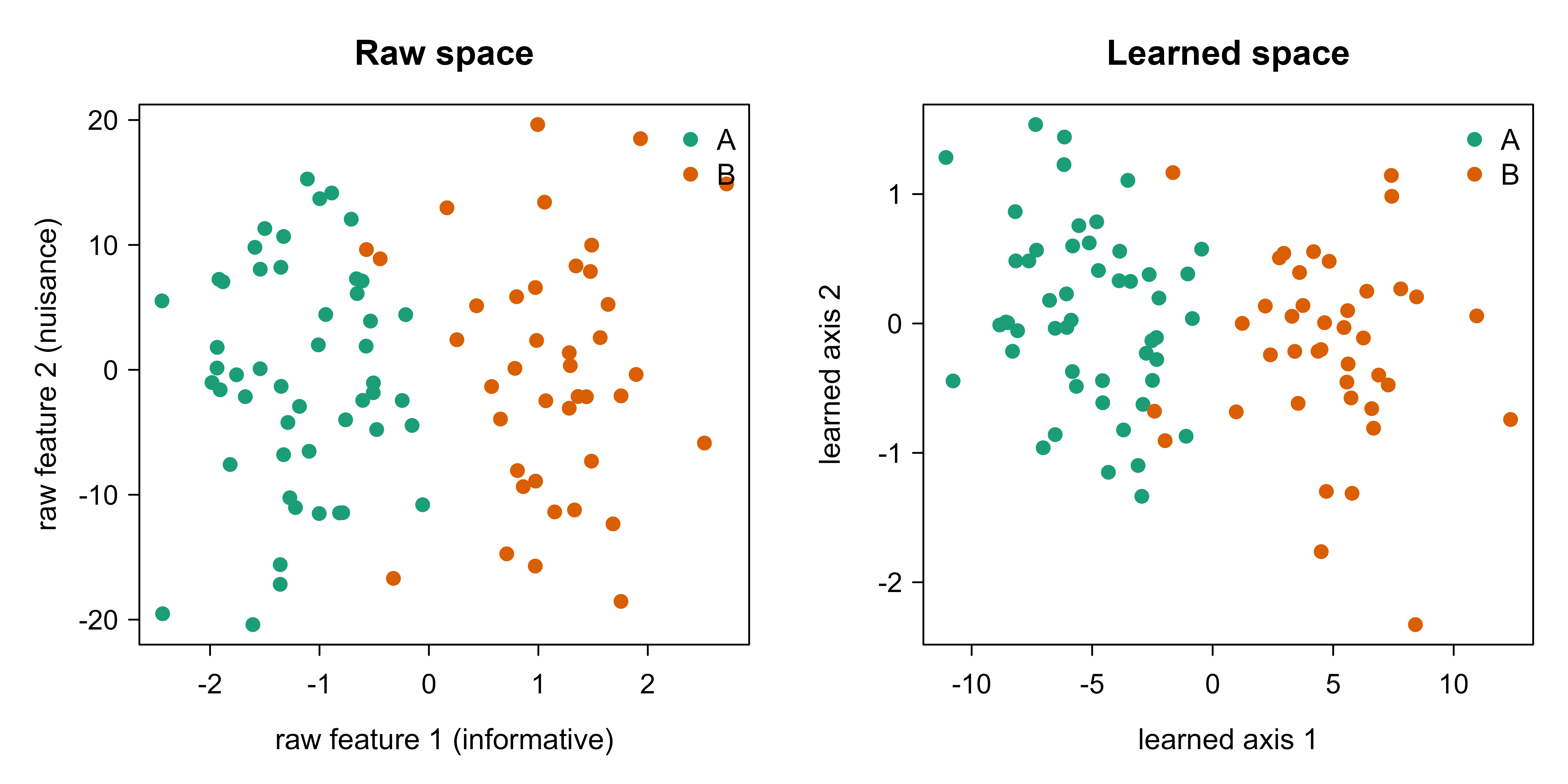
Figure 63.1 shows why the accuracy changes. The left panel plots the first two raw features: the classes overlap completely because the nuisance axis spreads both classes across the same range. The right panel plots the first two coordinates of the learned embedding \(z = Lx\), where the classes separate cleanly along the leading learned direction.

cols <- c(A = "#1b9e77", B = "#d95f02")
op <- par(mfrow = c(1, 2), mar = c(4, 4, 3, 1))

plot(Z_te_raw[, 1], Z_te_raw[, 2],
     col = cols[as.character(y_te)], pch = 19,
     xlab = "raw feature 1 (informative)", ylab = "raw feature 2 (nuisance)",
     main = "Raw space")
legend("topright", legend = names(cols), col = cols, pch = 19, bty = "n")

plot(Z_te_lrn[, 1], Z_te_lrn[, 2],
     col = cols[as.character(y_te)], pch = 19,
     xlab = "learned axis 1", ylab = "learned axis 2",
     main = "Learned space")
legend("topright", legend = names(cols), col = cols, pch = 19, bty = "n")

par(op)

Figure 63.1: Before and after the learned metric, on held-out test points. Left: the first two raw standardized features, where the high-variance nuisance axis (feature 2) buries the class structure and the two classes overlap. Right: the first two coordinates of the learned embedding z = Lx, where the metric has collapsed the nuisance directions and the classes separate along the leading learned axis. Same data, different ruler.

The lesson generalizes far beyond this toy: a model that fails for “stupid” reasons (scale, irrelevant features, correlated inputs) often needs a better metric, not a fancier classifier.

63.6 Verification and retrieval in practice

Once you have an embedding function, the two headline applications follow directly.

For verification, embed both inputs and threshold the distance: declare a match if \(D_{ij} \le \tau\). The threshold \(\tau\) is chosen on a validation set to hit a target operating point, trading off the false accept rate (impostors wrongly let in) against the false reject rate (genuine matches wrongly turned away). Because there is no per-identity output, the same model verifies identities it has never seen, which is the entire point for face unlock, speaker verification, and signature checking.

For retrieval, embed the whole gallery once and store the vectors. At query time, embed the query and return its nearest neighbors. With a few thousand items a brute-force scan is fine; at scale you index the embeddings with an approximate nearest-neighbor structure (see the embeddings and vector search chapter, Chapter 110) so lookups stay sublinear. The quality of retrieval is the quality of the metric: if similar items embed near each other, simple nearest-neighbor search is all you need on top.

A common refinement for both tasks is to L2-normalize the embeddings, mapping every vector to the unit sphere. Euclidean distance on the sphere is then a monotone function of cosine similarity, \(\lVert u - v \rVert^2 = 2 - 2\,u^\top v\) for unit vectors, so distance and cosine agree. Normalization removes embedding magnitude as a nuisance and is standard practice in face and text embedding systems.

The equivalence is exact, not approximate. For any vectors \(u,v\), expanding the squared norm gives \(\lVert u - v\rVert^2 = \lVert u\rVert^2 + \lVert v\rVert^2 - 2 u^\top v\). When both are unit vectors, \(\lVert u\rVert^2 = \lVert v\rVert^2 = 1\), so \(\lVert u - v\rVert^2 = 2 - 2\, u^\top v = 2(1 - \cos\angle(u,v))\). Squared Euclidean distance on the sphere is therefore an affine, strictly decreasing function of cosine similarity, which means any threshold on distance corresponds to an exactly equivalent threshold on cosine, and nearest-neighbor rankings under the two are identical. This is why face and text systems can train with cosine-based losses and retrieve with a Euclidean index, or vice versa, with no loss of information.

63.6.1 Verification as a decision problem

Verification with a threshold is a binary hypothesis test, and its theory tells you how to set \(\tau\). Let the genuine (same-identity) pair distances have density \(p_{\text{gen}}(D)\) and the impostor (different-identity) distances have density \(p_{\text{imp}}(D)\). Declaring a match when \(D \le \tau\) produces a false reject rate (a genuine pair called different) and a false accept rate (an impostor called the same), \[ \mathrm{FRR}(\tau) = \int_{\tau}^{\infty} p_{\text{gen}}(D)\, dD, \qquad \mathrm{FAR}(\tau) = \int_{0}^{\tau} p_{\text{imp}}(D)\, dD . \] Raising \(\tau\) admits more matches, which lowers FRR and raises FAR; the trade-off is the entire content of the detection-error or ROC curve, traced out as \(\tau\) varies. Two operating points are standard. The equal error rate (EER) is the \(\tau\) at which \(\mathrm{FRR}(\tau) = \mathrm{FAR}(\tau)\), a single summary number for comparing systems. For deployment you instead fix the tolerable FAR (say one impostor in \(10^4\)) and read off the \(\tau\) that achieves it, accepting whatever FRR results. Because the integrals depend on the densities and not on any closed label set, the same threshold generalizes to unseen identities, provided the validation distances are collected under deployment-matched conditions. The Bayes-optimal rule weights by the prior odds and costs: declare a match when the likelihood ratio \(p_{\text{gen}}(D)/p_{\text{imp}}(D)\) exceeds \(\frac{\pi_{\text{imp}}\, c_{\mathrm{FA}}}{\pi_{\text{gen}}\, c_{\mathrm{FR}}}\), where \(\pi\) are the priors and \(c\) the misclassification costs. When the two densities are unimodal with \(p_{\text{gen}}\) concentrated at small \(D\), this likelihood-ratio rule reduces to a single distance threshold, which is why thresholding works in practice.

Table 63.2 summarizes how the main approaches compare on the dimensions that matter when choosing one.

comp <- data.frame(
  Method = c("Mahalanobis (LMNN-style)", "Contrastive (siamese, 2 towers)",
             "Triplet (siamese, 3 towers)"),
  Supervision = c("class labels / pairs", "similar / dissimilar pairs",
                  "anchor-positive-negative triplets"),
  `Embedding map` = c("linear, z = Lx", "neural network f_theta",
                      "neural network f_theta"),
  `Open-set ready` = c("partly (linear capacity)", "yes", "yes"),
  `Main difficulty` = c("scales poorly with dimension",
                        "choosing the margin m",
                        "negative mining"),
  check.names = FALSE
)
knitr::kable(
  comp,
  caption = "Comparison of the metric-learning approaches covered in this chapter. Linear Mahalanobis methods are fast, convex, and interpretable but limited to linear geometry; deep contrastive and triplet methods handle complex data and open-set tasks at the cost of margin tuning and, for triplets, careful negative mining."
)

Table 63.2: Comparison of the metric-learning approaches covered in this chapter. Linear Mahalanobis methods are fast, convex, and interpretable but limited to linear geometry; deep contrastive and triplet methods handle complex data and open-set tasks at the cost of margin tuning and, for triplets, careful negative mining.

Method	Supervision	Embedding map	Open-set ready	Main difficulty
Mahalanobis (LMNN-style)	class labels / pairs	linear, z = Lx	partly (linear capacity)	scales poorly with dimension
Contrastive (siamese, 2 towers)	similar / dissimilar pairs	neural network f_theta	yes	choosing the margin m
Triplet (siamese, 3 towers)	anchor-positive-negative triplets	neural network f_theta	yes	negative mining

63.7 Practical guidance and pitfalls

The single most common mistake is information leakage through pairs. If you split your data into train and test by pairs rather than by identity, the same person can appear in both splits and your verification accuracy will be wildly optimistic. Always split by identity: every entity is wholly in train or wholly in test, so the test set genuinely measures generalization to unseen identities.

The second is collapse. A degenerate embedding that maps every input to the same point makes all similar pairs perfectly close and costs nothing on them. Contrastive and triplet losses guard against this with their margin term, which penalizes negatives that are too close, but a margin set too small or negatives that are too easy can still let the embedding drift toward collapse. Watch the spread of your embeddings during training, not just the loss.

Warning

With triplet loss, naive random sampling of negatives will stall training within a few epochs, because almost every random triplet already satisfies the margin and contributes no gradient. Budget engineering effort for semi-hard negative mining from the start; it is not an optional refinement but the difference between a model that learns and one that does not.

A few more field notes. Normalize or standardize raw features before learning a metric, since the whole exercise is about scale and an unstandardized feature will dominate the optimization for the wrong reason. Choose the embedding dimension \(k\) deliberately: smaller embeddings are faster to index and less prone to overfitting, but too small a \(k\) throws away discriminative structure. Calibrate the verification threshold on data that matches deployment conditions, because the right \(\tau\) depends on the base rate of genuine versus impostor pairs you will actually see. And remember that a learned metric inherits every bias in its training pairs: if certain groups are underrepresented in the “similar” pairs, the metric will serve them worse, which matters acutely for biometric verification.

When to use this

If a nearest-neighbor or clustering method underperforms and you suspect the distance is the problem (irrelevant features, mismatched scales, correlated inputs), a learned linear metric is a cheap, interpretable first move. Escalate to a deep siamese or triplet model when the geometry is genuinely nonlinear, the label set is open or huge, or you have only a handful of examples per class.

63.8 Connections

Metric learning sits between dimension reduction and classification and borrows from both. The linear case is a cousin of Fisher’s linear discriminant and of the supervised side of dimension reduction (Chapter 27). The deep case shares its losses with self-supervised contrastive learning (Chapter 49), where the “similar” pairs are two augmentations of the same image rather than two examples of the same labeled class, and the embeddings it produces are exactly the vectors consumed by the embeddings and vector search chapter (Chapter 110) for retrieval-augmented systems. The thread running through all of these is the same one this chapter opened with: when distance is the thing that matters, learn the distance.

63.9 Further reading

The foundational paper on supervised Mahalanobis metric learning is Weinberger and Saul, “Distance Metric Learning for Large Margin Nearest Neighbor Classification” (2009), which introduces the LMNN objective used here; the earlier Xing, Ng, Jordan, and Russell, “Distance Metric Learning, with Application to Clustering with Side-Information” (2002), sets up the pairwise-constraint formulation. For the deep side, Hadsell, Chopra, and LeCun, “Dimensionality Reduction by Learning an Invariant Mapping” (2006), introduces the contrastive loss and the siamese training setup, and Schroff, Kalenichenko, and Philbin, “FaceNet: A Unified Embedding for Face Recognition and Clustering” (2015), popularizes the triplet loss with semi-hard mining for large-scale verification. Bromley et al. (1993) is the original siamese-network paper, for signature verification. Kulis, “Metric Learning: A Survey” (2013), is a thorough and readable overview of the classical methods, and Bellet, Habrard, and Sebban, “A Survey on Metric Learning for Feature Vectors and Structured Data” (2015), is broader still. For the self-supervised contrastive descendants, see Chen, Kornblith, Norouzi, and Hinton, “A Simple Framework for Contrastive Learning of Visual Representations” (SimCLR, 2020).

---

1. Named for P. C. Mahalanobis, who introduced it in 1936 as a distance between a point and a distribution. Setting \(M\) to the inverse covariance of the data recovers his original statistical distance; metric learning generalizes the idea by fitting \(M\) to a supervised objective rather than to the data covariance.

2. This is closely related to Fisher’s linear discriminant and to Relevant Component Analysis (Bar-Hillel et al., 2003). The eigen-decomposition gives a global optimum in closed form, which is why it is ideal for a from-scratch demonstration; the iterative LMNN and deep variants trade the closed form for greater flexibility.