Advanced Data Analysis

Nguyen, Mike

7 Gaussian Process Regression

7.1 Latent Process Model

The object we are really after is the latent function. We model it as

\[ Y(x) = f(x) \]

where $f(x) \sim GP (m(x), c(x,x'))$ is a random process, specifically a Gaussian process, defined by two ingredients:

$m(x)$, the mean function, $m(x) = E[f(x)]$, which says where the function sits on average at each input.
$c(x,x')$, the covariance function, $c(x,x')= E[(f(x) - m(x)) (f(x') - m(x'))^T]$, which says how strongly the function values at two inputs $x$ and $x'$ move together.

These two functions play exactly the role that a mean vector and covariance matrix play for an ordinary multivariate normal, which brings us to a distinction that confuses many people the first time they meet it.

Intuition

The difference between a Gaussian distribution and a Gaussian process is the difference between a distribution over vectors and a distribution over functions.

Spelling that out:

A Gaussian distribution is a distribution over vectors. It is fully specified by a mean vector and a covariance matrix (for example, $\mathbf{Y} \sim N(\mathbf{\mu}, \mathbf{\Sigma})$, the familiar multivariate normal).
A Gaussian process is a distribution over functions. It is fully specified by a mean function $m$ and a covariance function $c$ (for example, $Y \sim GP(m,c)$). Once you supply those two functions, the GP is completely defined.

7.2 Gaussian Processes

A GP is an infinite-dimensional object: it assigns a joint distribution to the function values at every input location at once. That is what lets us make a prediction anywhere in our $x$ domain, provided we know the mean and covariance functions (the data-generating process). In particular, we need to be able to compute the covariance between any two $x$ locations.

Working with an infinite-dimensional object sounds intimidating, but in practice we never have to. Two facts rescue us:

We only ever have a finite set of data, and we only ever want predictions at a finite set of locations.
Any finite collection of GP random variables has a joint Gaussian distribution, that is, a multivariate normal distribution.

Key idea

This second fact is the defining property of a Gaussian process. It means every concrete calculation we do is a finite multivariate-normal calculation, even though the process itself is infinite-dimensional.

So all the work reduces to manipulating ordinary multivariate normals. The next section recalls the one result about multivariate normals that we will use over and over.

7.3 Gaussian Distributions

Suppose we stack two sets of jointly Gaussian variables, $\mathbf{v}$ and $\mathbf{v}_*$, into one vector. Their joint distribution is

\[ \left( \begin{array} {c} \mathbf{v} \\ \mathbf{v}_* \end{array} \right) \sim Gau \left( \left( \begin{array} {c} \mathbf{\mu} \\ \mathbf{\mu}_* \end{array} \right), \left( \begin{array} {cc} \mathbf{\Sigma} & \mathbf{\Sigma}_* \\ \mathbf{\Sigma}^T & \mathbf{\Sigma}_{**} \end{array} \right) \right) \]

where $E(\mathbf{v}) = \mathbf{\mu},E(\mathbf{v}_*) = \mathbf{\mu}_*, \mathbf{\Sigma}= cov(\mathbf{v}, \mathbf{v}), \mathbf{\Sigma}= cov(\mathbf{v}, \mathbf{v}_*),\mathbf{\Sigma}_{**} = cov(\mathbf{v}_*, \mathbf{v}_*)$.

The result we need is the conditional distribution of one block given the other. Partitioning the joint Gaussian gives

\[ \mathbf{v}_* | \mathbf{v} \sim Gau (\mathbf{\mu}_*+ \mathbf{\Sigma}^T_* \mathbf{\Sigma}^{-1} (\mathbf{v} - \mathbf{\mu}), \mathbf{\Sigma}_{**} - \mathbf{\Sigma}^T_* \mathbf{\Sigma}^{-1} \mathbf{\Sigma}_*) \]

Note

Read this formula slowly, because it is the engine of GP prediction. The conditional mean of $\mathbf{v}_*$ is its prior mean $\mathbf{\mu}_*$ plus a correction that pulls it toward the observed $\mathbf{v}$, weighted by how correlated the two blocks are. The conditional variance is the prior variance $\mathbf{\Sigma}_{**}$ reduced by an amount reflecting how much the observation explains. Observing $\mathbf{v}$ can only shrink our uncertainty about $\mathbf{v}_*$, never increase it.

With this single tool, GP prediction becomes a matter of identifying which quantities play the roles of $\mathbf{v}$ (the data) and $\mathbf{v}_*$ (the value we want to predict).

7.3.1 Deriving the conditioning formula

The conditional formula is so central that it is worth deriving rather than quoting. Write the joint precision (inverse covariance) matrix in block form and use the Schur complement. Let

\[ \mathbf{\Sigma} = \begin{pmatrix} \mathbf{\Sigma}_{vv} & \mathbf{\Sigma}_{v*} \\ \mathbf{\Sigma}_{*v} & \mathbf{\Sigma}_{**} \end{pmatrix}, \qquad \mathbf{S} \equiv \mathbf{\Sigma}_{**} - \mathbf{\Sigma}_{*v}\mathbf{\Sigma}_{vv}^{-1}\mathbf{\Sigma}_{v*} \tag{7.1}\]

where $\mathbf{S}$ is the Schur complement of the $\mathbf{\Sigma}_{vv}$ block. The block-matrix inverse is

\[ \mathbf{\Sigma}^{-1} = \begin{pmatrix} \mathbf{\Sigma}_{vv}^{-1} + \mathbf{\Sigma}_{vv}^{-1}\mathbf{\Sigma}_{v*}\mathbf{S}^{-1}\mathbf{\Sigma}_{*v}\mathbf{\Sigma}_{vv}^{-1} & -\mathbf{\Sigma}_{vv}^{-1}\mathbf{\Sigma}_{v*}\mathbf{S}^{-1} \\ -\mathbf{S}^{-1}\mathbf{\Sigma}_{*v}\mathbf{\Sigma}_{vv}^{-1} & \mathbf{S}^{-1} \end{pmatrix}. \tag{7.2}\]

The conditional density $p(\mathbf{v}_* \mid \mathbf{v})$ is proportional to the joint density viewed as a function of $\mathbf{v}_*$ with $\mathbf{v}$ held fixed. Expanding the quadratic form $-\tfrac{1}{2}(\cdot)^T\mathbf{\Sigma}^{-1}(\cdot)$ and collecting the terms in $\mathbf{v}_*$, the coefficient of the quadratic term is $\mathbf{S}^{-1}$ (the lower-right block of Equation 7.2), so the conditional covariance is $\mathbf{S}$. Completing the square in $\mathbf{v}_*$ identifies the conditional mean as the point where the linear term vanishes,

\[ E[\mathbf{v}_* \mid \mathbf{v}] = \mathbf{\mu}_* + \mathbf{\Sigma}_{*v}\mathbf{\Sigma}_{vv}^{-1}(\mathbf{v} - \mathbf{\mu}), \qquad \operatorname{cov}[\mathbf{v}_* \mid \mathbf{v}] = \mathbf{\Sigma}_{**} - \mathbf{\Sigma}_{*v}\mathbf{\Sigma}_{vv}^{-1}\mathbf{\Sigma}_{v*}. \tag{7.3}\]

Matching $\mathbf{\Sigma}_{*v} = \mathbf{\Sigma}_*^T$ recovers the formula stated above. Two facts fall out immediately. The conditional covariance does not depend on the observed value $\mathbf{v}$, only on the covariance structure, which is special to the Gaussian case. And because $\mathbf{S}$ is a Schur complement of a positive-definite matrix it is itself positive semi-definite, so $\mathbf{\Sigma}_{**} - \mathbf{\Sigma}_{*v}\mathbf{\Sigma}_{vv}^{-1}\mathbf{\Sigma}_{v*} \preceq \mathbf{\Sigma}_{**}$: conditioning never increases variance, confirming the claim in the callout above.

7.4 Optimal Linear Prediction

We want to predict $Y(x_0)$, the latent value at some arbitrary input $x_0$, given the data $\mathbf{z} \equiv (z_1, \dots, z_n)^T$. To keep things concrete, assume the mean function $\mu(x)$ is known for all $x$ (for instance, a constant).

Recall that we are looking for a linear predictor that minimizes the mean squared prediction error:

\[ \begin{aligned} \hat{Y} (x_0) &= k(x_0) + \sum_{i=1}^n w_i (x_0) z_i \\ &= k(x_0) + \mathbf{w}^T_0 \mathbf{z} \end{aligned} \]

A standard result is that the optimal linear predictor (under squared error) is also the conditional expectation $E(Y(x_0) |\mathbf{z})$. That is good news, because it means we do not have to solve a separate optimization problem: we can read the answer straight off the conditional distribution $Y(x_0) |\mathbf{z}$, using the multivariate-normal formula from the previous section.

7.4.1 Why the optimal weights are the conditioning weights

It is worth seeing directly that minimizing the mean squared prediction error reproduces the conditioning formula, since this is what justifies calling the conditional mean “optimal.” Take the mean function known and center the variables ($\mu_0 = 0$, $\mathbf{\mu} = \mathbf{0}$) without loss of generality, so the predictor is $\hat{Y}(x_0) = \mathbf{w}_0^T \mathbf{z}$. The objective is

\[ \text{MSPE}(\mathbf{w}_0) = E\!\left[(Y(x_0) - \mathbf{w}_0^T\mathbf{z})^2\right] = c_{0,0} - 2\,\mathbf{w}_0^T \mathbf{c}_0 + \mathbf{w}_0^T \mathbf{C}_z \mathbf{w}_0, \tag{7.4}\]

using $E[Y(x_0)^2] = c_{0,0}$, $E[Y(x_0)\mathbf{z}] = \mathbf{c}_0$, and $E[\mathbf{z}\mathbf{z}^T] = \mathbf{C}_z$. This is a strictly convex quadratic in $\mathbf{w}_0$ because $\mathbf{C}_z$ is positive definite. Setting the gradient to zero,

\[ \nabla_{\mathbf{w}_0}\,\text{MSPE} = -2\,\mathbf{c}_0 + 2\,\mathbf{C}_z \mathbf{w}_0 = \mathbf{0} \;\Longrightarrow\; \mathbf{w}_0 = \mathbf{C}_z^{-1}\mathbf{c}_0, \tag{7.5}\]

which is exactly the weight vector read off the conditional mean (this is the linear projection theorem; Equation 7.5 are the normal equations). Note that this derivation uses only second moments, not Gaussianity: $\mathbf{w}_0 = \mathbf{C}_z^{-1}\mathbf{c}_0$ is the best linear predictor for any process with these covariances. Gaussianity is what upgrades it to the best predictor among all functions of $\mathbf{z}$, since under joint normality the conditional expectation is linear and the two coincide. Substituting the optimal weights back into Equation 7.4 gives the minimized error

\[ \text{MSPE}(\mathbf{w}_0^\star) = c_{0,0} - \mathbf{c}_0^T \mathbf{C}_z^{-1}\mathbf{c}_0, \tag{7.6}\]

which is identical to the prediction variance $\sigma^2_{Y_0}$ derived from conditioning. The prediction variance is therefore not a separate quantity: it is the achieved mean squared error of the optimal predictor.

To apply that formula we first write the data model in vector form,

\[ \mathbf{z} = \mathbf{Y} + \epsilon, \epsilon \sim Gau(\mathbf{0}, \mathbf{C}_\epsilon) \]

where $\mathbf{Y}$ and $\epsilon$ are ordered in the same way as the data vector $\mathbf{z}$. We then collect the covariance pieces we will need. The covariance of the latent process at the observed locations is

\[ cov(\mathbf{Y}, \mathbf{Y}) \equiv \mathbf{C}_y \]

the covariance of the measurement errors is

\[ cov(\epsilon,\epsilon) \equiv \mathbf{C}_\epsilon \]

and because $Y$ and $\epsilon$ are independent, the covariance of the observations is the sum of the two:

\[ cov(\mathbf{z}, \mathbf{z}) = \mathbf{C}_y + \mathbf{C}_\epsilon \]

We also need the covariance between the target $Y(x_0)$ and the data, and the variance of the target itself:

\[ \mathbf{c}^T_0 \equiv cov( Y(x_0), \mathbf{z}) \]

\[ c_{0,0} \equiv var(Y(x_0)) \]

Here $\mu_0$ is the mean at $x_0$ and $\mathbf{\mu}$ is the mean vector corresponding to the observations. Writing $\mathbf{C}_z \equiv \mathbf{C}_y + \mathbf{C}_\epsilon$ for the observation covariance, the target and the data are jointly Gaussian:

\[ \left( \begin{array} {c} Y (x_0) \\ \mathbf{z} \end{array} \right) \sim Gau \left( \left( \begin{array} {c} \mu_0 \\ \mathbf{\mu} \end{array} \right), \left( \begin{array} {cc} c_{0,0} & \mathbf{c}^T_0 \\ \mathbf{c}_0 & \mathbf{C}_{z} \end{array} \right) \right) \]

Now we apply the joint/conditional Gaussian Distributions formula, matching $Y(x_0)$ to the block we want to predict and $\mathbf{z}$ to the block we condition on:

\[ Y(x_0)|\mathbf{z} \sim Gau (\mu_0+ \mathbf{c}^T_0 \mathbf{C}_z^{-1}(\mathbf{z}- \mathbf{\mu}), c_{0,0}- \mathbf{c}^T_0 \mathbf{C}_z^{-1} \mathbf{c}_0) \]

The predictor is the mean of this conditional distribution,

\[ \hat{Y}(x_0) = \mu_0 + \mathbf{c}_0^T \mathbf{C}^{-1}_z(\mathbf{z} - \mathbf{\mu}) \]

and the prediction variance is

\[ \sigma^2_{Y_0} = c_{0,0} - \mathbf{c}^T_0 \mathbf{C}_z^{-1} \mathbf{c}_0 \]

This predictor is optimal in the sense that it minimizes the mean squared prediction error,

\[ MSPE = E[(Y(x_0) - \hat{Y}(x_0))^2] \]

Comparing the predictor to the linear form we started with, we can now read off the weights and the constant. The weights are

\[ \mathbf{w}_0 = \mathbf{C}_z^{-1}\mathbf{c}_0 \]

and the constant is

\[ k(x_0) = \mu_0 - \mathbf{c}'_0 \mathbf{C}^{-1}_z \mathbf{\mu} \]

Intuition

The weights $\mathbf{w}_0$ form an effective kernel, just as in spline regression (Chapter 3) and local regression (Chapter 5). The prediction at $x_0$ is a weighted average of the observations, where each observation’s weight is determined by how covariant it is with the target (through $\mathbf{c}_0$) after accounting for how the observations covary with each other (through $\mathbf{C}_z^{-1}$). Points that are “close” to $x_0$, in the sense the covariance function defines, get more say.

These formulas extend directly to multiple prediction locations, with each location getting its own vector of weights.

Warning

The predictor requires the inverse $\mathbf{C}_z^{-1}$, an $n \times n$ matrix inversion that costs on the order of $n^3$ operations. With many sample locations this becomes the main computational bottleneck of GP regression, and a great deal of research is devoted to approximating it.

One special case is worth noting. When there are no measurement errors (so $z_i = y_i$), we simply replace $\mathbf{C}_z$ with $\mathbf{C}_y$ throughout. In that case the prediction at an observed location returns the observation exactly, with zero variance: the GP interpolates the data.

7.5 Covariance Functions

Everything above assumed we already knew the means and covariances. In practice we do not, and specifying them is where the real modeling happens. To predict at new $x$ locations we must supply two things:

a mean function (usually straightforward, often just a constant), and
a covariance function that returns a sensible value between any two locations (the hard part).

In the real world we hardly ever know the variances and covariances that fill in $\mathbf{C}_y, \mathbf{C}_\epsilon, \mathbf{c}_0, c_{0,0}$. The practical solution mirrors what we did for Linear Mixed Models (for example, AR and exponential models): we write the covariance function in terms of a few parameters $\mathbf{\theta}$ that can produce a covariance between any pair of coordinates, then estimate those parameters from data.

Not just any function will do. Two requirements shape the choice:

Covariance functions must be positive semi-definite. This guarantees that the prediction variances coming out of the formulas above are never negative, which would be nonsensical.
Covariance functions should be realistic, encoding the dependence structure we actually believe is present. This can be hard, but a simple and often sufficient assumption is that “nearby” observations (nearby in the same sense as kernel smoothing, Chapter 4) are more dependent than distant ones.

Tip

When in doubt, start from the principle that closeness in input space implies similarity in output. Almost every standard covariance function is just a different mathematical way of encoding that one idea.

To make estimation feasible we usually add a stationarity assumption. A process that is second-order (weakly) stationary has a constant expectation and a covariance that depends only on the separation between locations, $h = x - x'$, rather than on the locations themselves:

\[ c(x,x') = c(h, \mathbf{\theta}) \]

In two or more dimensions, if the dependence on the separation does not depend on direction (so it depends only on the distance $h = ||\mathbf{h}||$), the covariance function is called isotropic.

Stationarity buys us two practical advantages:

It allows a more parsimonious parameterization of the covariance function, since we estimate a function of distance rather than a separate value for every pair of locations.
It provides pseudo-replication of the dependence at each lag (many pairs of points share roughly the same separation), which gives estimation something to lean on.

When the inputs have more than one dimension, one classical way to build a valid covariance function is to multiply together valid one-dimensional pieces, giving a separable covariance function. For a two-dimensional input with coordinates $x_1$ and $x_2$,

\[ c(h_1;h_2) \equiv c(h_1) \times c_2(h_2) \]

which is a valid covariance as long as each factor is valid. Separability speeds up the matrix computations mentioned above, but it can be unrealistic for cases like spatio-temporal data, where space and time interact.

To get valid covariance functions in space and time, several families are commonly used. The most popular are listed here:

The Matern class, a flexible family with a parameter controlling smoothness.
The power exponential, $c(\tau, \theta) = \sigma^2 \exp \{ - \frac{|\tau|}{\theta} \}$, where $\sigma^2$ is the variance parameter and $\theta$ is the dependence (range) parameter that controls how quickly correlation decays with distance.
The Gaussian (squared-exponential) class, which produces very smooth functions.

7.5.1 Standard covariance functions, explicitly

It helps to have the common stationary families written out, with $r = \|x - x'\|$ the distance, $\sigma^2$ the marginal variance (signal scale), and $\ell > 0$ a length-scale (the same role as the range parameter $\theta$ above).

The squared-exponential (Gaussian, radial basis) kernel is

\[ c_{\text{SE}}(r) = \sigma^2 \exp\!\left(-\frac{r^2}{2\ell^2}\right). \tag{7.7}\]

It is infinitely differentiable, so sample paths are smooth ($C^\infty$). This smoothness is often unrealistically strong and makes the resulting $\mathbf{C}_z$ severely ill-conditioned, which is why a small “nugget” (a tiny $\sigma_\epsilon^2$ added to the diagonal) is almost always needed numerically even for deterministic data.

The Matern family interpolates between rough and smooth through an order parameter $\nu > 0$:

\[ c_{\nu}(r) = \sigma^2 \frac{2^{1-\nu}}{\Gamma(\nu)}\left(\frac{\sqrt{2\nu}\,r}{\ell}\right)^{\!\nu} K_\nu\!\left(\frac{\sqrt{2\nu}\,r}{\ell}\right), \tag{7.8}\]

where $K_\nu$ is the modified Bessel function of the second kind. The key structural fact is that a Matern-$\nu$ process is $\lceil \nu \rceil - 1$ times mean-square differentiable, so $\nu$ directly controls path smoothness. Half-integer $\nu$ gives closed forms that avoid the Bessel function: $\nu = 1/2$ recovers the exponential kernel $\sigma^2 e^{-r/\ell}$ (Ornstein-Uhlenbeck, continuous but nowhere differentiable paths); $\nu = 3/2$ gives $\sigma^2\big(1 + \tfrac{\sqrt{3}r}{\ell}\big)e^{-\sqrt{3}r/\ell}$; and $\nu \to \infty$ recovers the squared-exponential Equation 7.7. In spatial work $\nu = 3/2$ or $\nu = 5/2$ is a common, robust default because it avoids both the excessive smoothness of SE and the roughness of exponential.

The power-exponential family $c(r) = \sigma^2 \exp\{-(r/\theta)^p\}$ with $0 < p \le 2$ spans exponential ($p=1$) to Gaussian ($p=2$); the GPfit package used below fits exactly this form.

For multidimensional inputs with possibly different scales per coordinate, one uses an anisotropic (automatic relevance determination) version, for example

\[ c_{\text{SE-ARD}}(\mathbf{x},\mathbf{x}') = \sigma^2 \exp\!\left(-\tfrac{1}{2}\sum_{d=1}^{D}\frac{(x_d - x_d')^2}{\ell_d^2}\right), \tag{7.9}\]

where a large estimated $\ell_d$ means input $d$ is nearly irrelevant (its variations barely change the correlation), so the fitted length-scales double as a soft feature-selection diagnostic.

Positive definiteness, concretely

A function $c$ is a valid covariance if and only if the matrix $[c(x_i,x_j)]$ is positive semi-definite for every finite set of inputs. By Bochner’s theorem, a continuous stationary $c$ is positive definite exactly when it is the Fourier transform of a finite nonnegative measure (its spectral density). This is why you cannot freely invent covariance functions: the families above are precisely the ones with a valid spectral density.

7.5.2 The function-space prior and sampling from it

The conditioning view treats the GP as a tool for computing the predictor. The complementary function-space view makes the Bayesian reading explicit and is what underlies the “distribution over functions” slogan. Before seeing data, the prior over the latent function evaluated at any finite set of inputs $X = (x_1,\dots,x_m)$ is

\[ \mathbf{f} = (f(x_1),\dots,f(x_m))^T \sim N(\mathbf{m}, \mathbf{K}), \qquad K_{ij} = c(x_i, x_j). \tag{7.10}\]

A draw from this multivariate normal is a sampled function (evaluated on the grid $X$), and drawing several shows the prior’s typical wiggliness, set entirely by $c$. To draw such samples, factor $\mathbf{K} = \mathbf{L}\mathbf{L}^T$ (Cholesky) and set $\mathbf{f} = \mathbf{m} + \mathbf{L}\mathbf{u}$ with $\mathbf{u}\sim N(\mathbf{0},\mathbf{I})$; then $\operatorname{cov}(\mathbf{f}) = \mathbf{L}\mathbf{L}^T = \mathbf{K}$ as required. Conditioning Equation 7.10 on the noisy observations via Equation 7.3 turns these prior draws into posterior draws, which all pass near the data and fan out in the gaps, the function-space picture of the prediction band.

Once a family is chosen, the parameters of the covariance function (and of the mean function) have to be estimated. There are two main routes:

From a frequentist perspective, estimate the parameters with REML or MLE, exactly as in Linear Mixed Models, and predict the random process with BLUP.
From a Bayesian perspective, treat the GP on $f(x)$ as a prior distribution and update it with the observations $\mathbf{z}$ to get a posterior.

Warning

Whichever route you take, large numbers of data locations make estimation expensive, because of the same high-dimensional covariance matrices $\mathbf{C}_z, \mathbf{C}_y$ (and their inverses) that complicate prediction. Scaling GPs to large data sets is an active research area.

7.5.3 The marginal likelihood and how to optimize it

The standard frequentist (equivalently, empirical Bayes type-II maximum likelihood) route estimates the covariance parameters $\mathbf{\theta}$ by maximizing the marginal likelihood, the probability of the observed data with the latent function integrated out. Because $\mathbf{z} = \mathbf{Y} + \mathbf{\epsilon}$ is a sum of independent Gaussians, that integral is closed form: $\mathbf{z} \sim N(\mathbf{\mu}, \mathbf{C}_z)$ with $\mathbf{C}_z = \mathbf{C}_y(\mathbf{\theta}) + \sigma_\epsilon^2 \mathbf{I}$. Taking the mean known and centering, the log marginal likelihood is

\[ \log p(\mathbf{z}\mid\mathbf{\theta}) = -\tfrac{1}{2}\,\mathbf{z}^T \mathbf{C}_z^{-1}\mathbf{z} \;-\; \tfrac{1}{2}\log|\mathbf{C}_z| \;-\; \tfrac{n}{2}\log 2\pi . \tag{7.11}\]

The three terms have a clean reading. The data-fit term $-\tfrac{1}{2}\mathbf{z}^T\mathbf{C}_z^{-1}\mathbf{z}$ rewards covariance settings that explain the data; the complexity penalty $-\tfrac{1}{2}\log|\mathbf{C}_z|$ punishes overly flexible (large-determinant) covariances; and the constant fixes the normalization. The trade-off between these two is exactly Occam’s razor, and it is what lets the marginal likelihood select length-scales and noise levels without a separate validation set.

The gradient needed for optimization has a compact form. Writing $\mathbf{\alpha} = \mathbf{C}_z^{-1}\mathbf{z}$ and using $\partial \log|\mathbf{C}_z| = \operatorname{tr}(\mathbf{C}_z^{-1}\partial\mathbf{C}_z)$ together with $\partial \mathbf{C}_z^{-1} = -\mathbf{C}_z^{-1}(\partial\mathbf{C}_z)\mathbf{C}_z^{-1}$,

\[ \frac{\partial \log p(\mathbf{z}\mid\mathbf{\theta})}{\partial \theta_j} = \tfrac{1}{2}\,\operatorname{tr}\!\left[\left(\mathbf{\alpha}\mathbf{\alpha}^T - \mathbf{C}_z^{-1}\right)\frac{\partial \mathbf{C}_z}{\partial \theta_j}\right]. \tag{7.12}\]

These are plugged into a gradient-based optimizer (typically L-BFGS). One parameter admits a shortcut: the marginal variance $\sigma^2$ enters $\mathbf{C}_z$ as a multiplicative scale, so setting its derivative to zero gives the closed-form profile estimate $\hat{\sigma}^2 = \tfrac{1}{n}\mathbf{z}^T \mathbf{R}^{-1}\mathbf{z}$ where $\mathbf{R}$ is the correlation matrix (covariance with $\sigma^2$ factored out), reducing the dimension of the numerical search by one. REML differs from this by also integrating out the regression coefficients $\mathbf{\beta}$ of a parametric mean, which removes the downward bias in the variance and range estimates that plain MLE suffers in small samples, the same reason REML is preferred in linear mixed models.

Failure mode: a nonconvex surface

Equation 7.11 is generally not concave in $\mathbf{\theta}$ and can have multiple local optima with genuinely different interpretations, for example a “long length-scale, large noise” basin (the signal is a slow trend, the rest is noise) versus a “short length-scale, small noise” basin (the signal is wiggly and nearly noiseless). Restart the optimizer from several initializations and inspect which basin you land in rather than trusting a single run.

A few connections and special cases are worth keeping in mind:

If we model the mean function in terms of covariates, $\mu(x) = \mathbf{w}(x)'\mathbf{\beta}$ where $\mathbf{w}$ is a vector of covariates, the GP becomes a linear mixed model, with the one difference that the covariates must be available at any $x$ where we wish to predict.
When there is no measurement uncertainty ($\epsilon$), the prediction at an observed location equals the observation exactly. When there is measurement uncertainty, the GP instead filters it, smoothing through the noise.
We can also allow non-Gaussian observations conditioned on the GP, exactly as in a GLMM.

7.5.4 Connection to kernel ridge regression and RKHS

The GP posterior mean is not merely analogous to a kernel method, it is one. With a zero mean and homoscedastic noise $\mathbf{C}_z = \mathbf{K} + \sigma_\epsilon^2 \mathbf{I}$ (writing $\mathbf{K}$ for the kernel matrix of the latent process), the predictor Equation 7.3 becomes

\[ \hat{Y}(x_0) = \mathbf{k}_0^T (\mathbf{K} + \sigma_\epsilon^2 \mathbf{I})^{-1}\mathbf{z} = \sum_{i=1}^n \alpha_i\, c(x_0, x_i), \qquad \mathbf{\alpha} = (\mathbf{K} + \sigma_\epsilon^2\mathbf{I})^{-1}\mathbf{z}. \tag{7.13}\]

This is exactly the kernel ridge regression solution, where $\sigma_\epsilon^2$ plays the role of the ridge regularization parameter $\lambda$. The representer theorem explains why the predictor is a finite sum over training points despite living in an infinite-dimensional function space: the minimizer of the regularized loss $\sum_i (z_i - f(x_i))^2 + \lambda\|f\|_{\mathcal H}^2$ over the reproducing kernel Hilbert space $\mathcal H$ with kernel $c$ always has the form Equation 7.13. The GP adds what kernel ridge regression by itself does not provide: the predictive variance $\sigma^2_{Y_0}$ and a principled (marginal-likelihood) way to choose $\lambda = \sigma_\epsilon^2$ and the kernel parameters. There is also a weight-space view: if $c(x,x') = \phi(x)^T\phi(x')$ for a (possibly infinite) feature map $\phi$, then the GP is identical to Bayesian linear regression $f(x) = \phi(x)^T\mathbf{w}$ with prior $\mathbf{w}\sim N(\mathbf{0},\mathbf{I})$, and Equation 7.13 is the “kernel trick” applied to that regression.

7.5.5 Theoretical properties and failure modes

A few properties orient the method among its competitors. The posterior mean is the conditional expectation, hence unbiased for the latent value under the assumed model, but it shrinks toward the prior mean away from data, so its frequentist bias is nonzero whenever the true function leaves the prior’s typical set; the price of the honest variance is this prior-driven shrinkage. Posterior contraction results (van der Vaart and van Zanten) show that with a well-chosen kernel the posterior concentrates on the truth at near-minimax rates governed by the match between the kernel’s smoothness ($\nu$ for Matern) and the true function’s smoothness; a kernel that is too smooth oversmooths and a kernel that is too rough fails to borrow strength, both degrading the rate. Computationally, training costs $O(n^3)$ for the factorization and $O(n^2)$ memory for $\mathbf{C}_z$, and each prediction costs $O(n)$ for the mean and $O(n^2)$ for the variance after factorization. The dominant failure modes are: (i) numerical, when a too-smooth kernel or near-duplicate inputs make $\mathbf{C}_z$ ill-conditioned, cured by a nugget; (ii) misspecification, when stationarity is false (e.g. the function is smooth in one region and rough in another), which a single global length-scale cannot represent; and (iii) scale, the cubic cost, which motivates sparse/inducing-point approximations (Nystrom, FITC, variational SVGP) and structure-exploiting methods (Kronecker, KISS-GP) for large $n$.

When to use this

Reach for GP regression when you want smooth nonparametric predictions with honest uncertainty estimates, when your data set is small to moderate in size (so the $n^3$ cost is bearable), and when you have a sensible notion of which inputs should behave similarly. The design and analysis of computer experiments, where each “observation” is an expensive simulation run, is a classic fit.

With the theory assembled, we turn to a worked example.

7.5.6 Computing the predictor stably

In practice one never forms $\mathbf{C}_z^{-1}$ explicitly. The numerically stable recipe (Rasmussen and Williams, Algorithm 2.1) factors $\mathbf{C}_z = \mathbf{L}\mathbf{L}^T$ once with the Cholesky decomposition, then solves triangular systems:

\[ \mathbf{\alpha} = \mathbf{L}^T \backslash (\mathbf{L} \backslash \mathbf{z}), \qquad \hat{Y}(x_0) = \mathbf{c}_0^T \mathbf{\alpha}, \qquad \sigma^2_{Y_0} = c_{0,0} - \mathbf{w}^T\mathbf{w}\ \text{with}\ \mathbf{w} = \mathbf{L}\backslash\mathbf{c}_0, \tag{7.14}\]

where $\backslash$ denotes triangular solve. This is cheaper and far better conditioned than inversion, and it yields the log-determinant in Equation 7.11 for free as $\log|\mathbf{C}_z| = 2\sum_i \log L_{ii}$. If the Cholesky factorization fails, the cure is to add a small jitter (nugget) $\eta\mathbf{I}$ with $\eta$ a few orders of magnitude below the signal variance.

Verifying the formula numerically

The following short simulation confirms that the optimal-linear-predictor weights from Equation 7.5 reproduce the Cholesky-based predictor and that both match a brute-force least-squares solve, on a squared-exponential kernel.

Show code

set.seed(42)
n <- 12
xs <- sort(runif(n))
x0 <- 0.5
se <- function(a, b, l = 0.2, s2 = 1) s2 * exp(-outer(a, b, "-")^2 / (2 * l^2))
sig2 <- 0.01                            # observation noise
Cz <- se(xs, xs) + sig2 * diag(n)       # observation covariance
c0 <- as.numeric(se(x0, xs))            # cov(target, data)
z  <- sin(2 * pi * xs) + rnorm(n, sd = sqrt(sig2))

# (1) direct weights w0 = Cz^{-1} c0
yhat_direct <- as.numeric(crossprod(solve(Cz, c0), z))
# (2) Cholesky recipe
L <- chol(Cz)                           # upper-triangular: Cz = t(L) %*% L
alpha <- backsolve(L, forwardsolve(t(L), z))
yhat_chol <- sum(c0 * alpha)
c(direct = yhat_direct, cholesky = yhat_chol,
  diff = abs(yhat_direct - yhat_chol))
#>       direct     cholesky         diff 
#> 1.310350e-01 1.310350e-01 2.553513e-15

The two predictors agree to machine precision, confirming Equation 7.14 is just a stable rearrangement of Equation 7.5.

7.6 Application

This example uses the GPfit package; another option for fitting GP models is the mlegp package. The setup follows MacDonald, Ranjan, and Chipman (2015).

We will fit a GP to noiseless evaluations of a known test function,

\[ y(x) = \log(x + .1) + sin(5 \pi x) \]

so that we can compare the GP’s prediction to the truth. The function is wiggly enough to make the example interesting on the unit interval.

Rather than placing our few input points at random or on a uniform grid, we use a space-filling design. A Latin Hypercube design spreads points so that, projected onto any single input axis, they cover the range evenly. The Maximin version goes further by choosing the design that maximizes the minimum distance between points, which avoids clusters and gaps. Space-filling designs like these are the standard choice in the design of computer experiments, where each run is costly and we want every point to earn its keep.

We draw a small Maximin Latin Hypercube sample, evaluate the test function at those points, and fit the GP:

Show code

library(GPfit)
library(lhs)

set.seed(1)
n = 7
x = maximinLHS(n ,1) # draw a Maximin Latin Hypercube Sample
y = matrix(0, n, 1)
for (i in 1:n){
    y[i] = log(x[i] + .1 ) + sin(5*pi * x[i])
}

GPmodel = GP_fit(x,y)
print(GPmodel)
#> 
#> Number Of Observations: n = 7
#> Input Dimensions: d = 1
#> 
#> Correlation: Exponential (power = 1.95)
#> Correlation Parameters: 
#>     beta_hat
#> [1]  1.69817
#> 
#> sigma^2_hat: [1] 0.858342
#> 
#> delta_lb(beta_hat): [1] 0
#> 
#> nugget threshold parameter: 20

The printout reports the fitted correlation family (a power exponential), the estimated correlation parameter beta_hat (which controls how fast correlation decays with distance), and the estimated process variance sigma^2_hat. These are the $\mathbf{\theta}$ parameters of the covariance function, estimated from just seven points.

Next we predict on a dense grid across the input range and overlay the GP fit on the true function:

Show code

xvec <- seq(from = 0, to = 1, length.out = 100)
yvec <- matrix(0,100,1)
for (i in 1:100){
    yvec[i] = log(xvec[i] + .1) + sin(5*pi*xvec[i])
}
GPpred <- predict(GPmodel,xvec)

# data points are circles
# prediction is in the bllue
# 95% CIs (yhat + 2*s) are in red
plot(GPmodel, range= c(0,1), resolution = 100, colors = c("black","blue","red"), line_type = c(1,2),pch = 1)

# add the true function as a dotted black line
lines(xvec, yvec, col = "black", lty = 3)

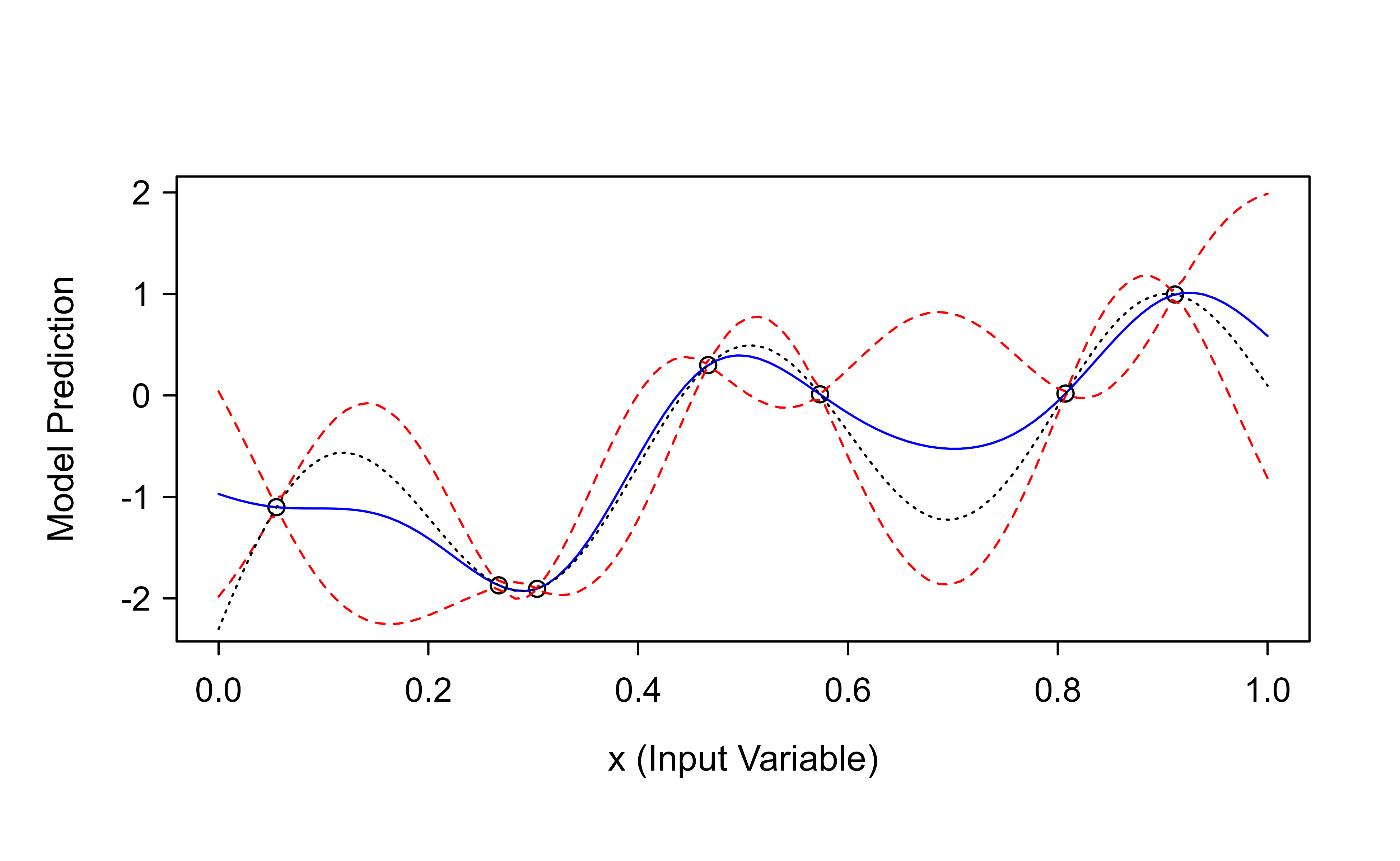
Figure 7.1: Gaussian process fit to seven noiseless evaluations of the test function. Circles are the design points, the blue dashed line is the posterior mean prediction, the red lines mark the approximate 95% prediction band, and the dotted black line is the true function.

Figure 7.1 overlays the fit on the truth. The circles are the seven design points, the blue dashed line is the GP’s posterior mean prediction, and the red lines mark the approximate 95% prediction band ($\hat{y} \pm 2s$). The dotted black line is the true function. Notice two things that bring the earlier theory to life. First, the blue prediction passes through (or nearly through) every data point: with noiseless observations the GP interpolates, exactly as the no-measurement-error case predicted. Second, the red band pinches tight near the data points and widens in the gaps between them, which is the conditional-variance formula at work: uncertainty shrinks where we have information and grows where we do not.

7.7 Takeaways

The chapter rests on a handful of ideas that are worth restating compactly:

A Gaussian process is a distribution over functions, defined by a mean function and a covariance function, with the property that any finite set of values from it is jointly multivariate normal.
Prediction is conditioning. Plugging the data and target into the multivariate-normal conditioning formula yields the optimal predictor $\hat{Y}(x_0) = \mu_0 + \mathbf{c}_0^T \mathbf{C}^{-1}_z(\mathbf{z} - \mathbf{\mu})$ and its variance $\sigma^2_{Y_0} = c_{0,0} - \mathbf{c}^T_0 \mathbf{C}_z^{-1} \mathbf{c}_0$ for free.
The covariance function is where the modeling lives. It must be positive semi-definite, and stationarity plus a small parametric family (Matern, power exponential, Gaussian) makes estimation tractable.
The price of all this flexibility and honest uncertainty is the $n \times n$ matrix inverse, which limits naive GPs to small and moderate data sets.

The independence assumption is the common starting point, but the framework extends naturally to correlated errors by giving them a non-diagonal covariance matrix.↩︎

# Gaussian Process Regression {#sec-gaussian-process-reg} ```{r} #| include: false source("_common.R") ``` Suggested reading: - @rasmussen2005 - @wikle2019 (section 4.2) Most of the regression methods in earlier chapters start by choosing a *form* for the function we want to learn: a line, a polynomial, a set of spline basis functions, a tree. Gaussian process (GP) regression takes a different starting point. Instead of committing to a particular functional form, we place a probability distribution directly over functions, and then let the data tell us which functions are plausible. The result is a flexible, nonparametric method that not only predicts a value at any new input but also reports how uncertain that prediction is. The intuition is worth pausing on before any math. Imagine you have measured an unknown function at a handful of input locations. A GP says: "before seeing the data, I believe the underlying function is smooth, and that points close together in input space should have similar output values." Once the data arrive, the GP keeps only the functions consistent with what was observed, and from that shrunken collection it forms a prediction (the average of the surviving functions) and a measure of confidence (how much those functions still disagree). Where you have data, the predictions are confident; where you do not, the uncertainty grows. This honest accounting of uncertainty is one of the main reasons GPs are popular in fields like spatial statistics, the design and analysis of computer experiments, and Bayesian optimization (a workhorse of hyperparameter optimization, @sec-hyperparameter-optimization). In this chapter you will learn what a Gaussian process is and how it differs from an ordinary Gaussian distribution, how the conditioning formula for the multivariate normal gives us a closed-form predictor and prediction variance, why the choice of *covariance function* is the heart of the method, and how to fit a GP in R. The mathematical machinery turns out to be a single, reusable idea: any finite set of values from a GP is jointly multivariate normal, so prediction reduces to conditioning one part of a Gaussian on another. ::: {.callout-important title="Key idea"} A Gaussian process is a distribution over functions. Prediction with a GP is nothing more than conditioning a (very large) multivariate normal distribution on the values we have observed. ::: We begin with the model that connects what we observe to the latent function we want to recover. Under a Gaussian Process (GP), we assume that $Y$ is a random (Gaussian) process that is controlled by a mean function and a covariance function. We rarely observe $Y$ directly; instead we observe noisy measurements of it. The response model writes each observation $z_i$ as the latent value $Y_i$ plus measurement error: $$ z_i = Y_i + \epsilon_i, i = 1, \dots, n $$ This model rests on three assumptions: - $Y$ is a latent process specified by a GP. - The $\epsilon_i$ are independent and identically distributed mean-zero observation errors, independent of $Y$, with variance $\sigma_\epsilon^2$. - The errors are assumed to be normal (Gaussian), $\epsilon_i \sim iid N (0, \sigma^2_\epsilon)$.^[The independence assumption is the common starting point, but the framework extends naturally to correlated errors by giving them a non-diagonal covariance matrix.] With the model in place, the natural question is how to turn observed $z_i$ values into a prediction at a new location $x_0$. We start with the simplest sensible candidate: a linear predictor, meaning a prediction built as a weighted sum of the data, $$ \hat{Y}(x_0) = k_0 + \sum_{i=1}^n w_i z_i $$ where the $w_i$ are weights and $k_0$ is a constant. The whole problem now reduces to choosing good weights. We will pick "optimal" weights in the mean-squared-error sense, and doing that forces us to think carefully about the random process that controls $Y$. The next sections build up exactly the probabilistic structure we need. ## Latent Process Model The object we are really after is the latent function. We model it as $$ Y(x) = f(x) $$ where $f(x) \sim GP (m(x), c(x,x'))$ is a random process, specifically a Gaussian process, defined by two ingredients: - $m(x)$, the mean function, $m(x) = E[f(x)]$, which says where the function sits on average at each input. - $c(x,x')$, the covariance function, $c(x,x')= E[(f(x) - m(x)) (f(x') - m(x'))^T]$, which says how strongly the function values at two inputs $x$ and $x'$ move together. These two functions play exactly the role that a mean vector and covariance matrix play for an ordinary multivariate normal, which brings us to a distinction that confuses many people the first time they meet it. ::: {.callout-tip title="Intuition"} The difference between a Gaussian *distribution* and a Gaussian *process* is the difference between a distribution over vectors and a distribution over functions. ::: Spelling that out: - A Gaussian distribution is a distribution over vectors. It is fully specified by a mean vector and a covariance matrix (for example, $\mathbf{Y} \sim N(\mathbf{\mu}, \mathbf{\Sigma})$, the familiar multivariate normal). - A Gaussian process is a distribution over functions. It is fully specified by a mean function $m$ and a covariance function $c$ (for example, $Y \sim GP(m,c)$). Once you supply those two functions, the GP is completely defined. ## Gaussian Processes A GP is an infinite-dimensional object: it assigns a joint distribution to the function values at *every* input location at once. That is what lets us make a prediction anywhere in our $x$ domain, provided we know the mean and covariance functions (the data-generating process). In particular, we need to be able to compute the covariance between *any* two $x$ locations. Working with an infinite-dimensional object sounds intimidating, but in practice we never have to. Two facts rescue us: - We only ever have a finite set of data, and we only ever want predictions at a finite set of locations. - Any finite collection of GP random variables has a joint Gaussian distribution, that is, a multivariate normal distribution. ::: {.callout-important title="Key idea"} This second fact is the defining property of a Gaussian process. It means every concrete calculation we do is a finite multivariate-normal calculation, even though the process itself is infinite-dimensional. ::: So all the work reduces to manipulating ordinary multivariate normals. The next section recalls the one result about multivariate normals that we will use over and over. ## Gaussian Distributions Suppose we stack two sets of jointly Gaussian variables, $\mathbf{v}$ and $\mathbf{v}_*$, into one vector. Their joint distribution is $$ \left( \begin{array} {c} \mathbf{v} \\ \mathbf{v}_* \end{array} \right) \sim Gau \left( \left( \begin{array} {c} \mathbf{\mu} \\ \mathbf{\mu}_* \end{array} \right), \left( \begin{array} {cc} \mathbf{\Sigma} & \mathbf{\Sigma}_* \\ \mathbf{\Sigma}^T & \mathbf{\Sigma}_{**} \end{array} \right) \right) $$ where $E(\mathbf{v}) = \mathbf{\mu},E(\mathbf{v}_*) = \mathbf{\mu}_*, \mathbf{\Sigma}= cov(\mathbf{v}, \mathbf{v}), \mathbf{\Sigma}= cov(\mathbf{v}, \mathbf{v}_*),\mathbf{\Sigma}_{**} = cov(\mathbf{v}_*, \mathbf{v}_*)$. The result we need is the conditional distribution of one block given the other. Partitioning the joint Gaussian gives $$ \mathbf{v}_* | \mathbf{v} \sim Gau (\mathbf{\mu}_*+ \mathbf{\Sigma}^T_* \mathbf{\Sigma}^{-1} (\mathbf{v} - \mathbf{\mu}), \mathbf{\Sigma}_{**} - \mathbf{\Sigma}^T_* \mathbf{\Sigma}^{-1} \mathbf{\Sigma}_*) $$ ::: {.callout-note} Read this formula slowly, because it is the engine of GP prediction. The conditional mean of $\mathbf{v}_*$ is its prior mean $\mathbf{\mu}_*$ plus a correction that pulls it toward the observed $\mathbf{v}$, weighted by how correlated the two blocks are. The conditional variance is the prior variance $\mathbf{\Sigma}_{**}$ *reduced* by an amount reflecting how much the observation explains. Observing $\mathbf{v}$ can only shrink our uncertainty about $\mathbf{v}_*$, never increase it. ::: With this single tool, GP prediction becomes a matter of identifying which quantities play the roles of $\mathbf{v}$ (the data) and $\mathbf{v}_*$ (the value we want to predict). ### Deriving the conditioning formula {#sec-gaussian-process-reg-conditioning-derivation} The conditional formula is so central that it is worth deriving rather than quoting. Write the joint precision (inverse covariance) matrix in block form and use the Schur complement. Let $$ \mathbf{\Sigma} = \begin{pmatrix} \mathbf{\Sigma}_{vv} & \mathbf{\Sigma}_{v*} \\ \mathbf{\Sigma}_{*v} & \mathbf{\Sigma}_{**} \end{pmatrix}, \qquad \mathbf{S} \equiv \mathbf{\Sigma}_{**} - \mathbf{\Sigma}_{*v}\mathbf{\Sigma}_{vv}^{-1}\mathbf{\Sigma}_{v*} $$ {#eq-gaussian-process-reg-schur} where $\mathbf{S}$ is the Schur complement of the $\mathbf{\Sigma}_{vv}$ block. The block-matrix inverse is $$ \mathbf{\Sigma}^{-1} = \begin{pmatrix} \mathbf{\Sigma}_{vv}^{-1} + \mathbf{\Sigma}_{vv}^{-1}\mathbf{\Sigma}_{v*}\mathbf{S}^{-1}\mathbf{\Sigma}_{*v}\mathbf{\Sigma}_{vv}^{-1} & -\mathbf{\Sigma}_{vv}^{-1}\mathbf{\Sigma}_{v*}\mathbf{S}^{-1} \\ -\mathbf{S}^{-1}\mathbf{\Sigma}_{*v}\mathbf{\Sigma}_{vv}^{-1} & \mathbf{S}^{-1} \end{pmatrix}. $$ {#eq-gaussian-process-reg-blockinv} The conditional density $p(\mathbf{v}_* \mid \mathbf{v})$ is proportional to the joint density viewed as a function of $\mathbf{v}_*$ with $\mathbf{v}$ held fixed. Expanding the quadratic form $-\tfrac{1}{2}(\cdot)^T\mathbf{\Sigma}^{-1}(\cdot)$ and collecting the terms in $\mathbf{v}_*$, the coefficient of the quadratic term is $\mathbf{S}^{-1}$ (the lower-right block of @eq-gaussian-process-reg-blockinv), so the conditional covariance is $\mathbf{S}$. Completing the square in $\mathbf{v}_*$ identifies the conditional mean as the point where the linear term vanishes, $$ E[\mathbf{v}_* \mid \mathbf{v}] = \mathbf{\mu}_* + \mathbf{\Sigma}_{*v}\mathbf{\Sigma}_{vv}^{-1}(\mathbf{v} - \mathbf{\mu}), \qquad \operatorname{cov}[\mathbf{v}_* \mid \mathbf{v}] = \mathbf{\Sigma}_{**} - \mathbf{\Sigma}_{*v}\mathbf{\Sigma}_{vv}^{-1}\mathbf{\Sigma}_{v*}. $$ {#eq-gaussian-process-reg-condderived} Matching $\mathbf{\Sigma}_{*v} = \mathbf{\Sigma}_*^T$ recovers the formula stated above. Two facts fall out immediately. The conditional covariance does not depend on the observed value $\mathbf{v}$, only on the covariance structure, which is special to the Gaussian case. And because $\mathbf{S}$ is a Schur complement of a positive-definite matrix it is itself positive semi-definite, so $\mathbf{\Sigma}_{**} - \mathbf{\Sigma}_{*v}\mathbf{\Sigma}_{vv}^{-1}\mathbf{\Sigma}_{v*} \preceq \mathbf{\Sigma}_{**}$: conditioning never increases variance, confirming the claim in the callout above. ## Optimal Linear Prediction We want to predict $Y(x_0)$, the latent value at some arbitrary input $x_0$, given the data $\mathbf{z} \equiv (z_1, \dots, z_n)^T$. To keep things concrete, assume the mean function $\mu(x)$ is known for all $x$ (for instance, a constant). Recall that we are looking for a linear predictor that minimizes the mean squared prediction error: $$ \begin{aligned} \hat{Y} (x_0) &= k(x_0) + \sum_{i=1}^n w_i (x_0) z_i \\ &= k(x_0) + \mathbf{w}^T_0 \mathbf{z} \end{aligned} $$ A standard result is that the optimal linear predictor (under squared error) is also the conditional expectation $E(Y(x_0) |\mathbf{z})$. That is good news, because it means we do not have to solve a separate optimization problem: we can read the answer straight off the conditional distribution $Y(x_0) |\mathbf{z}$, using the multivariate-normal formula from the previous section. ### Why the optimal weights are the conditioning weights {#sec-gaussian-process-reg-optimal-weights} It is worth seeing directly that minimizing the mean squared prediction error reproduces the conditioning formula, since this is what justifies calling the conditional mean "optimal." Take the mean function known and center the variables ($\mu_0 = 0$, $\mathbf{\mu} = \mathbf{0}$) without loss of generality, so the predictor is $\hat{Y}(x_0) = \mathbf{w}_0^T \mathbf{z}$. The objective is $$ \text{MSPE}(\mathbf{w}_0) = E\!\left[(Y(x_0) - \mathbf{w}_0^T\mathbf{z})^2\right] = c_{0,0} - 2\,\mathbf{w}_0^T \mathbf{c}_0 + \mathbf{w}_0^T \mathbf{C}_z \mathbf{w}_0, $$ {#eq-gaussian-process-reg-mspe-quad} using $E[Y(x_0)^2] = c_{0,0}$, $E[Y(x_0)\mathbf{z}] = \mathbf{c}_0$, and $E[\mathbf{z}\mathbf{z}^T] = \mathbf{C}_z$. This is a strictly convex quadratic in $\mathbf{w}_0$ because $\mathbf{C}_z$ is positive definite. Setting the gradient to zero, $$ \nabla_{\mathbf{w}_0}\,\text{MSPE} = -2\,\mathbf{c}_0 + 2\,\mathbf{C}_z \mathbf{w}_0 = \mathbf{0} \;\Longrightarrow\; \mathbf{w}_0 = \mathbf{C}_z^{-1}\mathbf{c}_0, $$ {#eq-gaussian-process-reg-normal-eq} which is exactly the weight vector read off the conditional mean (this is the linear projection theorem; @eq-gaussian-process-reg-normal-eq are the normal equations). Note that this derivation uses only second moments, not Gaussianity: $\mathbf{w}_0 = \mathbf{C}_z^{-1}\mathbf{c}_0$ is the best *linear* predictor for any process with these covariances. Gaussianity is what upgrades it to the best predictor among all functions of $\mathbf{z}$, since under joint normality the conditional expectation is linear and the two coincide. Substituting the optimal weights back into @eq-gaussian-process-reg-mspe-quad gives the minimized error $$ \text{MSPE}(\mathbf{w}_0^\star) = c_{0,0} - \mathbf{c}_0^T \mathbf{C}_z^{-1}\mathbf{c}_0, $$ {#eq-gaussian-process-reg-mspe-min} which is identical to the prediction variance $\sigma^2_{Y_0}$ derived from conditioning. The prediction variance is therefore not a separate quantity: it *is* the achieved mean squared error of the optimal predictor. To apply that formula we first write the data model in vector form, $$ \mathbf{z} = \mathbf{Y} + \epsilon, \epsilon \sim Gau(\mathbf{0}, \mathbf{C}_\epsilon) $$ where $\mathbf{Y}$ and $\epsilon$ are ordered in the same way as the data vector $\mathbf{z}$. We then collect the covariance pieces we will need. The covariance of the latent process at the observed locations is $$ cov(\mathbf{Y}, \mathbf{Y}) \equiv \mathbf{C}_y $$ the covariance of the measurement errors is $$ cov(\epsilon,\epsilon) \equiv \mathbf{C}_\epsilon $$ and because $Y$ and $\epsilon$ are independent, the covariance of the *observations* is the sum of the two: $$ cov(\mathbf{z}, \mathbf{z}) = \mathbf{C}_y + \mathbf{C}_\epsilon $$ We also need the covariance between the target $Y(x_0)$ and the data, and the variance of the target itself: $$ \mathbf{c}^T_0 \equiv cov( Y(x_0), \mathbf{z}) $$ $$ c_{0,0} \equiv var(Y(x_0)) $$ Here $\mu_0$ is the mean at $x_0$ and $\mathbf{\mu}$ is the mean vector corresponding to the observations. Writing $\mathbf{C}_z \equiv \mathbf{C}_y + \mathbf{C}_\epsilon$ for the observation covariance, the target and the data are jointly Gaussian: $$ \left( \begin{array} {c} Y (x_0) \\ \mathbf{z} \end{array} \right) \sim Gau \left( \left( \begin{array} {c} \mu_0 \\ \mathbf{\mu} \end{array} \right), \left( \begin{array} {cc} c_{0,0} & \mathbf{c}^T_0 \\ \mathbf{c}_0 & \mathbf{C}_{z} \end{array} \right) \right) $$ Now we apply the joint/conditional [Gaussian Distributions] formula, matching $Y(x_0)$ to the block we want to predict and $\mathbf{z}$ to the block we condition on: $$ Y(x_0)|\mathbf{z} \sim Gau (\mu_0+ \mathbf{c}^T_0 \mathbf{C}_z^{-1}(\mathbf{z}- \mathbf{\mu}), c_{0,0}- \mathbf{c}^T_0 \mathbf{C}_z^{-1} \mathbf{c}_0) $$ The predictor is the mean of this conditional distribution, $$ \hat{Y}(x_0) = \mu_0 + \mathbf{c}_0^T \mathbf{C}^{-1}_z(\mathbf{z} - \mathbf{\mu}) $$ and the prediction variance is $$ \sigma^2_{Y_0} = c_{0,0} - \mathbf{c}^T_0 \mathbf{C}_z^{-1} \mathbf{c}_0 $$ This predictor is optimal in the sense that it minimizes the mean squared prediction error, $$ MSPE = E[(Y(x_0) - \hat{Y}(x_0))^2] $$ Comparing the predictor to the linear form we started with, we can now read off the weights and the constant. The weights are $$ \mathbf{w}_0 = \mathbf{C}_z^{-1}\mathbf{c}_0 $$ and the constant is $$ k(x_0) = \mu_0 - \mathbf{c}'_0 \mathbf{C}^{-1}_z \mathbf{\mu} $$ ::: {.callout-tip title="Intuition"} The weights $\mathbf{w}_0$ form an *effective kernel*, just as in spline regression (@sec-spline) and local regression (@sec-local). The prediction at $x_0$ is a weighted average of the observations, where each observation's weight is determined by how covariant it is with the target (through $\mathbf{c}_0$) after accounting for how the observations covary with each other (through $\mathbf{C}_z^{-1}$). Points that are "close" to $x_0$, in the sense the covariance function defines, get more say. ::: These formulas extend directly to multiple prediction locations, with each location getting its own vector of weights. ::: {.callout-warning} The predictor requires the inverse $\mathbf{C}_z^{-1}$, an $n \times n$ matrix inversion that costs on the order of $n^3$ operations. With many sample locations this becomes the main computational bottleneck of GP regression, and a great deal of research is devoted to approximating it. ::: One special case is worth noting. When there are no measurement errors (so $z_i = y_i$), we simply replace $\mathbf{C}_z$ with $\mathbf{C}_y$ throughout. In that case the prediction at an observed location returns the observation exactly, with zero variance: the GP interpolates the data. ## Covariance Functions Everything above assumed we already knew the means and covariances. In practice we do not, and specifying them is where the real modeling happens. To predict at new $x$ locations we must supply two things: 1. a mean function (usually straightforward, often just a constant), and 2. a covariance function that returns a sensible value between *any* two locations (the hard part). In the real world we hardly ever know the variances and covariances that fill in $\mathbf{C}_y, \mathbf{C}_\epsilon, \mathbf{c}_0, c_{0,0}$. The practical solution mirrors what we did for [Linear Mixed Models](https://bookdown.org/mike/data_analysis/linear-mixed-models.html) (for example, AR and exponential models): we write the covariance function in terms of a few parameters $\mathbf{\theta}$ that can produce a covariance between any pair of coordinates, then estimate those parameters from data. Not just any function will do. Two requirements shape the choice: - Covariance functions must be positive semi-definite. This guarantees that the prediction variances coming out of the formulas above are never negative, which would be nonsensical. - Covariance functions should be realistic, encoding the dependence structure we actually believe is present. This can be hard, but a simple and often sufficient assumption is that "nearby" observations (nearby in the same sense as kernel smoothing, @sec-kernel) are more dependent than distant ones. ::: {.callout-tip} When in doubt, start from the principle that closeness in input space implies similarity in output. Almost every standard covariance function is just a different mathematical way of encoding that one idea. ::: To make estimation feasible we usually add a stationarity assumption. A process that is second-order (weakly) stationary has a constant expectation and a covariance that depends only on the *separation* between locations, $h = x - x'$, rather than on the locations themselves: $$ c(x,x') = c(h, \mathbf{\theta}) $$ In two or more dimensions, if the dependence on the separation does not depend on direction (so it depends only on the distance $h = ||\mathbf{h}||$), the covariance function is called isotropic. Stationarity buys us two practical advantages: - It allows a more parsimonious parameterization of the covariance function, since we estimate a function of distance rather than a separate value for every pair of locations. - It provides pseudo-replication of the dependence at each lag (many pairs of points share roughly the same separation), which gives estimation something to lean on. When the inputs have more than one dimension, one classical way to build a valid covariance function is to multiply together valid one-dimensional pieces, giving a separable covariance function. For a two-dimensional input with coordinates $x_1$ and $x_2$, $$ c(h_1;h_2) \equiv c(h_1) \times c_2(h_2) $$ which is a valid covariance as long as each factor is valid. Separability speeds up the matrix computations mentioned above, but it can be unrealistic for cases like spatio-temporal data, where space and time interact. To get valid covariance functions in space and time, several families are commonly used. The most popular are listed here: - The Matern class, a flexible family with a parameter controlling smoothness. - The power exponential, $c(\tau, \theta) = \sigma^2 \exp \{ - \frac{|\tau|}{\theta} \}$, where $\sigma^2$ is the variance parameter and $\theta$ is the dependence (range) parameter that controls how quickly correlation decays with distance. - The Gaussian (squared-exponential) class, which produces very smooth functions. ### Standard covariance functions, explicitly {#sec-gaussian-process-reg-cov-explicit} It helps to have the common stationary families written out, with $r = \|x - x'\|$ the distance, $\sigma^2$ the marginal variance (signal scale), and $\ell > 0$ a length-scale (the same role as the range parameter $\theta$ above). The squared-exponential (Gaussian, radial basis) kernel is $$ c_{\text{SE}}(r) = \sigma^2 \exp\!\left(-\frac{r^2}{2\ell^2}\right). $$ {#eq-gaussian-process-reg-se} It is infinitely differentiable, so sample paths are smooth ($C^\infty$). This smoothness is often unrealistically strong and makes the resulting $\mathbf{C}_z$ severely ill-conditioned, which is why a small "nugget" (a tiny $\sigma_\epsilon^2$ added to the diagonal) is almost always needed numerically even for deterministic data. The Matern family interpolates between rough and smooth through an order parameter $\nu > 0$: $$ c_{\nu}(r) = \sigma^2 \frac{2^{1-\nu}}{\Gamma(\nu)}\left(\frac{\sqrt{2\nu}\,r}{\ell}\right)^{\!\nu} K_\nu\!\left(\frac{\sqrt{2\nu}\,r}{\ell}\right), $$ {#eq-gaussian-process-reg-matern} where $K_\nu$ is the modified Bessel function of the second kind. The key structural fact is that a Matern-$\nu$ process is $\lceil \nu \rceil - 1$ times mean-square differentiable, so $\nu$ directly controls path smoothness. Half-integer $\nu$ gives closed forms that avoid the Bessel function: $\nu = 1/2$ recovers the exponential kernel $\sigma^2 e^{-r/\ell}$ (Ornstein-Uhlenbeck, continuous but nowhere differentiable paths); $\nu = 3/2$ gives $\sigma^2\big(1 + \tfrac{\sqrt{3}r}{\ell}\big)e^{-\sqrt{3}r/\ell}$; and $\nu \to \infty$ recovers the squared-exponential @eq-gaussian-process-reg-se. In spatial work $\nu = 3/2$ or $\nu = 5/2$ is a common, robust default because it avoids both the excessive smoothness of SE and the roughness of exponential. The power-exponential family $c(r) = \sigma^2 \exp\{-(r/\theta)^p\}$ with $0 < p \le 2$ spans exponential ($p=1$) to Gaussian ($p=2$); the `GPfit` package used below fits exactly this form. For multidimensional inputs with possibly different scales per coordinate, one uses an anisotropic (automatic relevance determination) version, for example $$ c_{\text{SE-ARD}}(\mathbf{x},\mathbf{x}') = \sigma^2 \exp\!\left(-\tfrac{1}{2}\sum_{d=1}^{D}\frac{(x_d - x_d')^2}{\ell_d^2}\right), $$ {#eq-gaussian-process-reg-ard} where a large estimated $\ell_d$ means input $d$ is nearly irrelevant (its variations barely change the correlation), so the fitted length-scales double as a soft feature-selection diagnostic. ::: {.callout-note title="Positive definiteness, concretely"} A function $c$ is a valid covariance if and only if the matrix $[c(x_i,x_j)]$ is positive semi-definite for every finite set of inputs. By Bochner's theorem, a continuous stationary $c$ is positive definite exactly when it is the Fourier transform of a finite nonnegative measure (its spectral density). This is why you cannot freely invent covariance functions: the families above are precisely the ones with a valid spectral density. ::: ### The function-space prior and sampling from it {#sec-gaussian-process-reg-function-space} The conditioning view treats the GP as a tool for computing the predictor. The complementary function-space view makes the Bayesian reading explicit and is what underlies the "distribution over functions" slogan. Before seeing data, the prior over the latent function evaluated at any finite set of inputs $X = (x_1,\dots,x_m)$ is $$ \mathbf{f} = (f(x_1),\dots,f(x_m))^T \sim N(\mathbf{m}, \mathbf{K}), \qquad K_{ij} = c(x_i, x_j). $$ {#eq-gaussian-process-reg-prior} A draw from this multivariate normal is a sampled function (evaluated on the grid $X$), and drawing several shows the prior's typical wiggliness, set entirely by $c$. To draw such samples, factor $\mathbf{K} = \mathbf{L}\mathbf{L}^T$ (Cholesky) and set $\mathbf{f} = \mathbf{m} + \mathbf{L}\mathbf{u}$ with $\mathbf{u}\sim N(\mathbf{0},\mathbf{I})$; then $\operatorname{cov}(\mathbf{f}) = \mathbf{L}\mathbf{L}^T = \mathbf{K}$ as required. Conditioning @eq-gaussian-process-reg-prior on the noisy observations via @eq-gaussian-process-reg-condderived turns these prior draws into posterior draws, which all pass near the data and fan out in the gaps, the function-space picture of the prediction band. Once a family is chosen, the parameters of the covariance function (and of the mean function) have to be estimated. There are two main routes: 1. From a frequentist perspective, estimate the parameters with REML or MLE, exactly as in [Linear Mixed Models](https://bookdown.org/mike/data_analysis/linear-mixed-models.html), and predict the random process with BLUP. 2. From a Bayesian perspective, treat the GP on $f(x)$ as a prior distribution and update it with the observations $\mathbf{z}$ to get a posterior. ::: {.callout-warning} Whichever route you take, large numbers of data locations make estimation expensive, because of the same high-dimensional covariance matrices $\mathbf{C}_z, \mathbf{C}_y$ (and their inverses) that complicate prediction. Scaling GPs to large data sets is an active research area. ::: ### The marginal likelihood and how to optimize it {#sec-gaussian-process-reg-marginal-likelihood} The standard frequentist (equivalently, empirical Bayes type-II maximum likelihood) route estimates the covariance parameters $\mathbf{\theta}$ by maximizing the marginal likelihood, the probability of the observed data with the latent function integrated out. Because $\mathbf{z} = \mathbf{Y} + \mathbf{\epsilon}$ is a sum of independent Gaussians, that integral is closed form: $\mathbf{z} \sim N(\mathbf{\mu}, \mathbf{C}_z)$ with $\mathbf{C}_z = \mathbf{C}_y(\mathbf{\theta}) + \sigma_\epsilon^2 \mathbf{I}$. Taking the mean known and centering, the log marginal likelihood is $$ \log p(\mathbf{z}\mid\mathbf{\theta}) = -\tfrac{1}{2}\,\mathbf{z}^T \mathbf{C}_z^{-1}\mathbf{z} \;-\; \tfrac{1}{2}\log|\mathbf{C}_z| \;-\; \tfrac{n}{2}\log 2\pi . $$ {#eq-gaussian-process-reg-logml} The three terms have a clean reading. The data-fit term $-\tfrac{1}{2}\mathbf{z}^T\mathbf{C}_z^{-1}\mathbf{z}$ rewards covariance settings that explain the data; the complexity penalty $-\tfrac{1}{2}\log|\mathbf{C}_z|$ punishes overly flexible (large-determinant) covariances; and the constant fixes the normalization. The trade-off between these two is exactly Occam's razor, and it is what lets the marginal likelihood select length-scales and noise levels without a separate validation set. The gradient needed for optimization has a compact form. Writing $\mathbf{\alpha} = \mathbf{C}_z^{-1}\mathbf{z}$ and using $\partial \log|\mathbf{C}_z| = \operatorname{tr}(\mathbf{C}_z^{-1}\partial\mathbf{C}_z)$ together with $\partial \mathbf{C}_z^{-1} = -\mathbf{C}_z^{-1}(\partial\mathbf{C}_z)\mathbf{C}_z^{-1}$, $$ \frac{\partial \log p(\mathbf{z}\mid\mathbf{\theta})}{\partial \theta_j} = \tfrac{1}{2}\,\operatorname{tr}\!\left[\left(\mathbf{\alpha}\mathbf{\alpha}^T - \mathbf{C}_z^{-1}\right)\frac{\partial \mathbf{C}_z}{\partial \theta_j}\right]. $$ {#eq-gaussian-process-reg-mlgrad} These are plugged into a gradient-based optimizer (typically L-BFGS). One parameter admits a shortcut: the marginal variance $\sigma^2$ enters $\mathbf{C}_z$ as a multiplicative scale, so setting its derivative to zero gives the closed-form profile estimate $\hat{\sigma}^2 = \tfrac{1}{n}\mathbf{z}^T \mathbf{R}^{-1}\mathbf{z}$ where $\mathbf{R}$ is the correlation matrix (covariance with $\sigma^2$ factored out), reducing the dimension of the numerical search by one. REML differs from this by also integrating out the regression coefficients $\mathbf{\beta}$ of a parametric mean, which removes the downward bias in the variance and range estimates that plain MLE suffers in small samples, the same reason REML is preferred in linear mixed models. ::: {.callout-warning title="Failure mode: a nonconvex surface"} @eq-gaussian-process-reg-logml is generally not concave in $\mathbf{\theta}$ and can have multiple local optima with genuinely different interpretations, for example a "long length-scale, large noise" basin (the signal is a slow trend, the rest is noise) versus a "short length-scale, small noise" basin (the signal is wiggly and nearly noiseless). Restart the optimizer from several initializations and inspect which basin you land in rather than trusting a single run. ::: A few connections and special cases are worth keeping in mind: - If we model the mean function in terms of covariates, $\mu(x) = \mathbf{w}(x)'\mathbf{\beta}$ where $\mathbf{w}$ is a vector of covariates, the GP becomes a [linear mixed model](https://bookdown.org/mike/data_analysis/linear-mixed-models.html), with the one difference that the covariates must be available at *any* $x$ where we wish to predict. - When there is no measurement uncertainty ($\epsilon$), the prediction at an observed location equals the observation exactly. When there is measurement uncertainty, the GP instead filters it, smoothing through the noise. - We can also allow non-Gaussian observations conditioned on the GP, exactly as in a [GLMM](https://bookdown.org/mike/data_analysis/nonlinear-and-generalized-linear-mixed-models.html). ### Connection to kernel ridge regression and RKHS {#sec-gaussian-process-reg-krr} The GP posterior mean is not merely analogous to a kernel method, it is one. With a zero mean and homoscedastic noise $\mathbf{C}_z = \mathbf{K} + \sigma_\epsilon^2 \mathbf{I}$ (writing $\mathbf{K}$ for the kernel matrix of the latent process), the predictor @eq-gaussian-process-reg-condderived becomes $$ \hat{Y}(x_0) = \mathbf{k}_0^T (\mathbf{K} + \sigma_\epsilon^2 \mathbf{I})^{-1}\mathbf{z} = \sum_{i=1}^n \alpha_i\, c(x_0, x_i), \qquad \mathbf{\alpha} = (\mathbf{K} + \sigma_\epsilon^2\mathbf{I})^{-1}\mathbf{z}. $$ {#eq-gaussian-process-reg-krr} This is exactly the kernel ridge regression solution, where $\sigma_\epsilon^2$ plays the role of the ridge regularization parameter $\lambda$. The representer theorem explains why the predictor is a finite sum over training points despite living in an infinite-dimensional function space: the minimizer of the regularized loss $\sum_i (z_i - f(x_i))^2 + \lambda\|f\|_{\mathcal H}^2$ over the reproducing kernel Hilbert space $\mathcal H$ with kernel $c$ always has the form @eq-gaussian-process-reg-krr. The GP adds what kernel ridge regression by itself does not provide: the predictive variance $\sigma^2_{Y_0}$ and a principled (marginal-likelihood) way to choose $\lambda = \sigma_\epsilon^2$ and the kernel parameters. There is also a weight-space view: if $c(x,x') = \phi(x)^T\phi(x')$ for a (possibly infinite) feature map $\phi$, then the GP is identical to Bayesian linear regression $f(x) = \phi(x)^T\mathbf{w}$ with prior $\mathbf{w}\sim N(\mathbf{0},\mathbf{I})$, and @eq-gaussian-process-reg-krr is the "kernel trick" applied to that regression. ### Theoretical properties and failure modes {#sec-gaussian-process-reg-theory} A few properties orient the method among its competitors. The posterior mean is the conditional expectation, hence unbiased for the latent value under the assumed model, but it shrinks toward the prior mean away from data, so its frequentist bias is nonzero whenever the true function leaves the prior's typical set; the price of the honest variance is this prior-driven shrinkage. Posterior contraction results (van der Vaart and van Zanten) show that with a well-chosen kernel the posterior concentrates on the truth at near-minimax rates governed by the match between the kernel's smoothness ($\nu$ for Matern) and the true function's smoothness; a kernel that is too smooth oversmooths and a kernel that is too rough fails to borrow strength, both degrading the rate. Computationally, training costs $O(n^3)$ for the factorization and $O(n^2)$ memory for $\mathbf{C}_z$, and each prediction costs $O(n)$ for the mean and $O(n^2)$ for the variance after factorization. The dominant failure modes are: (i) numerical, when a too-smooth kernel or near-duplicate inputs make $\mathbf{C}_z$ ill-conditioned, cured by a nugget; (ii) misspecification, when stationarity is false (e.g. the function is smooth in one region and rough in another), which a single global length-scale cannot represent; and (iii) scale, the cubic cost, which motivates sparse/inducing-point approximations (Nystrom, FITC, variational SVGP) and structure-exploiting methods (Kronecker, KISS-GP) for large $n$. ::: {.callout-tip title="When to use this"} Reach for GP regression when you want smooth nonparametric predictions *with* honest uncertainty estimates, when your data set is small to moderate in size (so the $n^3$ cost is bearable), and when you have a sensible notion of which inputs should behave similarly. The design and analysis of computer experiments, where each "observation" is an expensive simulation run, is a classic fit. ::: With the theory assembled, we turn to a worked example. ### Computing the predictor stably {#sec-gaussian-process-reg-cholesky} In practice one never forms $\mathbf{C}_z^{-1}$ explicitly. The numerically stable recipe (Rasmussen and Williams, Algorithm 2.1) factors $\mathbf{C}_z = \mathbf{L}\mathbf{L}^T$ once with the Cholesky decomposition, then solves triangular systems: $$ \mathbf{\alpha} = \mathbf{L}^T \backslash (\mathbf{L} \backslash \mathbf{z}), \qquad \hat{Y}(x_0) = \mathbf{c}_0^T \mathbf{\alpha}, \qquad \sigma^2_{Y_0} = c_{0,0} - \mathbf{w}^T\mathbf{w}\ \text{with}\ \mathbf{w} = \mathbf{L}\backslash\mathbf{c}_0, $$ {#eq-gaussian-process-reg-cholpred} where $\backslash$ denotes triangular solve. This is cheaper and far better conditioned than inversion, and it yields the log-determinant in @eq-gaussian-process-reg-logml for free as $\log|\mathbf{C}_z| = 2\sum_i \log L_{ii}$. If the Cholesky factorization fails, the cure is to add a small jitter (nugget) $\eta\mathbf{I}$ with $\eta$ a few orders of magnitude below the signal variance. ::: {.callout-tip title="Verifying the formula numerically"} The following short simulation confirms that the optimal-linear-predictor weights from @eq-gaussian-process-reg-normal-eq reproduce the Cholesky-based predictor and that both match a brute-force least-squares solve, on a squared-exponential kernel. ```{r} set.seed(42) n <- 12 xs <- sort(runif(n)) x0 <- 0.5 se <- function(a, b, l = 0.2, s2 = 1) s2 * exp(-outer(a, b, "-")^2 / (2 * l^2)) sig2 <- 0.01 # observation noise Cz <- se(xs, xs) + sig2 * diag(n) # observation covariance c0 <- as.numeric(se(x0, xs)) # cov(target, data) z <- sin(2 * pi * xs) + rnorm(n, sd = sqrt(sig2)) # (1) direct weights w0 = Cz^{-1} c0 yhat_direct <- as.numeric(crossprod(solve(Cz, c0), z)) # (2) Cholesky recipe L <- chol(Cz) # upper-triangular: Cz = t(L) %*% L alpha <- backsolve(L, forwardsolve(t(L), z)) yhat_chol <- sum(c0 * alpha) c(direct = yhat_direct, cholesky = yhat_chol, diff = abs(yhat_direct - yhat_chol)) ``` The two predictors agree to machine precision, confirming @eq-gaussian-process-reg-cholpred is just a stable rearrangement of @eq-gaussian-process-reg-normal-eq. ::: ## Application This example uses the `GPfit` package; another option for fitting GP models is the `mlegp` package. The setup follows @macdonald2015. We will fit a GP to noiseless evaluations of a known test function, $$ y(x) = \log(x + .1) + sin(5 \pi x) $$ so that we can compare the GP's prediction to the truth. The function is wiggly enough to make the example interesting on the unit interval. Rather than placing our few input points at random or on a uniform grid, we use a space-filling design. A Latin Hypercube design spreads points so that, projected onto any single input axis, they cover the range evenly. The Maximin version goes further by choosing the design that maximizes the minimum distance between points, which avoids clusters and gaps. Space-filling designs like these are the standard choice in the design of computer experiments, where each run is costly and we want every point to earn its keep. We draw a small Maximin Latin Hypercube sample, evaluate the test function at those points, and fit the GP: ```{r} library(GPfit) library(lhs) set.seed(1) n = 7 x = maximinLHS(n ,1) # draw a Maximin Latin Hypercube Sample y = matrix(0, n, 1) for (i in 1:n){ y[i] = log(x[i] + .1 ) + sin(5*pi * x[i]) } GPmodel = GP_fit(x,y) print(GPmodel) ``` The printout reports the fitted correlation family (a power exponential), the estimated correlation parameter `beta_hat` (which controls how fast correlation decays with distance), and the estimated process variance `sigma^2_hat`. These are the $\mathbf{\theta}$ parameters of the covariance function, estimated from just seven points. Next we predict on a dense grid across the input range and overlay the GP fit on the true function: ```{r fig-gaussian-process-reg-fit-vs-truth, fig.cap="Gaussian process fit to seven noiseless evaluations of the test function. Circles are the design points, the blue dashed line is the posterior mean prediction, the red lines mark the approximate 95% prediction band, and the dotted black line is the true function."} xvec <- seq(from = 0, to = 1, length.out = 100) yvec <- matrix(0,100,1) for (i in 1:100){ yvec[i] = log(xvec[i] + .1) + sin(5*pi*xvec[i]) } GPpred <- predict(GPmodel,xvec) # data points are circles # prediction is in the bllue # 95% CIs (yhat + 2*s) are in red plot(GPmodel, range= c(0,1), resolution = 100, colors = c("black","blue","red"), line_type = c(1,2),pch = 1) # add the true function as a dotted black line lines(xvec, yvec, col = "black", lty = 3) ``` @fig-gaussian-process-reg-fit-vs-truth overlays the fit on the truth. The circles are the seven design points, the blue dashed line is the GP's posterior mean prediction, and the red lines mark the approximate 95% prediction band ($\hat{y} \pm 2s$). The dotted black line is the true function. Notice two things that bring the earlier theory to life. First, the blue prediction passes through (or nearly through) every data point: with noiseless observations the GP interpolates, exactly as the no-measurement-error case predicted. Second, the red band pinches tight near the data points and widens in the gaps between them, which is the conditional-variance formula at work: uncertainty shrinks where we have information and grows where we do not. ## Takeaways The chapter rests on a handful of ideas that are worth restating compactly: - A Gaussian process is a distribution over functions, defined by a mean function and a covariance function, with the property that any finite set of values from it is jointly multivariate normal. - Prediction is conditioning. Plugging the data and target into the multivariate-normal conditioning formula yields the optimal predictor $\hat{Y}(x_0) = \mu_0 + \mathbf{c}_0^T \mathbf{C}^{-1}_z(\mathbf{z} - \mathbf{\mu})$ and its variance $\sigma^2_{Y_0} = c_{0,0} - \mathbf{c}^T_0 \mathbf{C}_z^{-1} \mathbf{c}_0$ for free. - The covariance function is where the modeling lives. It must be positive semi-definite, and stationarity plus a small parametric family (Matern, power exponential, Gaussian) makes estimation tractable. - The price of all this flexibility and honest uncertainty is the $n \times n$ matrix inverse, which limits naive GPs to small and moderate data sets.