Advanced Data Analysis

Nguyen, Mike

31 Multidimensional Scaling and Nonlinear Dimension Reduction

Imagine you are handed a table of distances between thirty cities, but no map. Could you reconstruct a map from the distances alone? Multidimensional scaling answers yes: given only how far apart things are, it places them as points in a low-dimensional space (say, two dimensions you can plot) so that the plotted distances match the given ones as closely as possible. The same idea works for any data where you can measure how similar or dissimilar pairs of observations are, even when “distance” means something subjective like how alike two products feel to a customer.

This chapter introduces two families of methods that share that goal. The first, multidimensional scaling (MDS), is a classical, mostly linear approach: it tries to preserve all pairwise distances at once. The second, nonlinear dimension reduction (also called manifold learning), assumes the data actually live on a curved, lower-dimensional surface sitting inside the high-dimensional space, and tries to “unroll” that surface. By the end you will know what each method optimizes, how the pieces fit together, and when one is preferable to another. These methods complement the linear techniques such as PCA covered in the dimension reduction chapter (Chapter 27); here we relax the assumption that the structure we want is a flat subspace.

Key idea

All the methods in this chapter take a notion of closeness between observations and find a low-dimensional placement of points that keeps close things close. They differ in which closeness they insist on preserving (global vs. local) and in how flexible the placement is allowed to be (linear vs. nonlinear).

31.1 Multidimensional Scaling

In multidimensional scaling, the main objective is to represent the original observations in a lower-dimensional space such that the “distortion” due to the dimension reduction is minimized. That is, we expect the similarity or dissimilarity between pairs of observations to remain as close as possible after we reduce the dimensionality.

We can pursue this goal in two different settings. The first uses actual metrics, that is, numerical distances. The second uses only non-metric rank orders of the pairwise relationships: for a set of observed similarities or distances between every pair of observations, we seek a presentation of the observations in as few dimensions as possible so that the new proximities nearly match the original proximities, but we ask only that the ordering of proximities be respected rather than their exact values.

The technique has two historical homes. In classical multivariate statistics, multidimensional scaling is used as a way to visually represent multi-dimensional data, often reducing to two or three dimensions so a human can inspect the result. In modern statistical learning applications, it is often used as a means of presenting observations in lower dimensional spaces for further modeling or analysis, where the reduced coordinates become features fed into a downstream algorithm.

Let us set up notation. Consider observations $x_1, \dots, x_n \in R^p$. Let $d_{ij}$ be the distance between observations $i$ and $j$. This distance could be Euclidean distance, $d_{ij} =||x_i - x_j||$, but it can also be more general (e.g., any of the Minkowski distances, or perhaps just some general dissimilarity measure, even a subjective measure of how close the two observations are to each other).¹

So, in multidimensional scaling (MDS), we seek values $z_i, \dots, z_n \in R^k$ ($k <p$) to minimize a stress function.²

Intuition

Think of the $z_i$ as pins you are free to slide around on a corkboard, and the $d_{ii'}$ as target distances printed on a list. The stress function scores how badly your current pin layout violates the target list. MDS slides the pins until the score is as low as it can go.

31.1.1 Metric Scalings

In metric scaling the distances $d_{ii'}$ are genuine numbers we want to reproduce. The three variants below differ only in how they weigh the errors and in whether they work from distances or from similarities.

31.1.1.1 Kruskal-Shepard

The most direct stress function simply sums the squared gaps between original and reduced distances,

\[ S_M(z_1, z_2, \dots, z_n) = \sum_{i \neq i'} (d_{ii'} - ||z_i - z_{i'}||)^2 \]

which is called least squares or Kruskal-Shepard scaling. In words, we want the pairwise distance between the new lower dimensional variables $z_i$ and $z_{i'}$ to be as close as possible to the distance in the original dimension, $d_{ii'}$.

This minimization is not analytical but can be solved computationally by a gradient descent algorithm.³

The gradient is worth writing out, both because it drives the algorithm and because it exposes the geometry. Differentiating $S_M$ with respect to a single point $z_i$, and using $\partial \|z_i - z_{i'}\| / \partial z_i = (z_i - z_{i'})/\|z_i - z_{i'}\|$, gives

\[ \frac{\partial S_M}{\partial z_i} = -4 \sum_{i' \neq i} \big(d_{ii'} - \|z_i - z_{i'}\|\big)\, \frac{z_i - z_{i'}}{\|z_i - z_{i'}\|} . \tag{31.1}\]

Each term is a spring: the unit vector $(z_i - z_{i'})/\|z_i - z_{i'}\|$ points along the edge, and the scalar $d_{ii'} - \|z_i - z_{i'}\|$ is positive when the points are currently too close (pull apart) and negative when too far (push together). The configuration is in equilibrium when these spring forces balance at every point. A practical consequence of Equation 31.1 is the singularity at $z_i = z_{i'}$: coincident points produce an undefined direction, so implementations either perturb ties or, more robustly, use the SMACOF majorization algorithm (Scaling by MAjorizing a COmplicated Function), which replaces the non-smooth stress by a quadratic upper bound at each iteration and so guarantees a monotone, divide-free decrease of stress.

31.1.1.2 Sammon Mapping

A variation of least squares scaling is the Sammon mapping, which minimizes

\[ S_{S_m}(z_1, z_2, \dots, z_n) = \sum_{i \neq i'} \frac{(d_{ii'} - ||z_i - z_{i'}||)^2}{d_{ii'}} \]

The only change from Kruskal-Shepard is the $d_{ii'}$ in the denominator, but it matters: dividing by the original distance makes a fixed error count for more when the pair is close together. As a result the Sammon mapping preserves smaller pairwise distances more-so than larger distances.

When to use this

Reach for the Sammon mapping over plain least squares when the fine-grained structure among nearby points matters more to you than getting the gross, large-scale distances exactly right.

31.1.1.3 Classical Scaling

A third stress function is called classical scaling, where we start with similarities $s_{ii'}$ rather than distances. Typically, one uses the centered inner product similarity $s_{ii'} = <x_i - \bar{x}, x_{i'} - \bar{x}>$. In this case, we minimize

\[ S_C (z_1, \dots, z_n) = \sum_{i \neq i'} (s_{ii'} - <z_i - \bar{z}, z_{i'} - \bar{z}>)^2 \]

Unlike the previous two, this can be solved explicitly in terms of an eigen-decomposition, so no iterative search is needed. In fact, in this context one can show an equivalence between MDS and PCA.⁴

Note

This equivalence is reassuring but also a limitation. Because classical scaling is PCA in disguise, it can only capture linear structure. The nonlinear methods later in the chapter exist precisely to go beyond what an eigen-decomposition of a centered similarity matrix can see.

31.1.1.3.1 Derivation: from distances to coordinates by double centering

The remarkable fact about classical scaling is that we can recover coordinates from distances alone, with no iterative search, provided the distances are Euclidean. Suppose the $d_{ii'}$ arise as Euclidean distances from some unknown centered configuration, $d_{ii'}^2 = \|x_i - x_{i'}\|^2$. Expand the square,

\[ d_{ii'}^2 = \|x_i\|^2 + \|x_{i'}\|^2 - 2\, x_i^\top x_{i'} . \tag{31.2}\]

Write $b_{ii'} = x_i^\top x_{i'}$ for the (centered) Gram matrix entry. The squared-distance matrix mixes the wanted inner products $b_{ii'}$ with the unwanted diagonal terms $\|x_i\|^2$ and $\|x_{i'}\|^2$. Those unwanted terms are constant along rows and columns, so they can be annihilated by double centering: subtract the row mean, the column mean, and add back the grand mean. Define the centering matrix

\[ \mathbf{H} = \mathbf{I} - \tfrac{1}{n}\mathbf{1}\mathbf{1}^\top , \tag{31.3}\]

and let $\mathbf{D}^{(2)}$ be the matrix with entries $d_{ii'}^2$. Applying Equation 31.2 and using $\sum_i x_i = 0$ (the configuration is centered), the row and column means of $\mathbf{D}^{(2)}$ exactly capture the $\|x_i\|^2$ terms, and one obtains the key identity

\[ \mathbf{B} = -\tfrac{1}{2}\,\mathbf{H}\,\mathbf{D}^{(2)}\,\mathbf{H} = \mathbf{X}\mathbf{X}^\top , \tag{31.4}\]

so that $b_{ii'} = x_i^\top x_{i'}$. The double-centered squared-distance matrix is the centered Gram matrix. Since $\mathbf{B}$ is symmetric positive semidefinite of rank at most $p$, take its spectral decomposition $\mathbf{B} = \mathbf{U}\boldsymbol{\Lambda}\mathbf{U}^\top$ with $\lambda_1 \ge \lambda_2 \ge \cdots \ge 0$. The classical-scaling coordinates in $k$ dimensions are the leading scaled eigenvectors,

\[ \mathbf{Z} = \mathbf{U}_k \boldsymbol{\Lambda}_k^{1/2}, \qquad z_i = \big(\sqrt{\lambda_1}\,u_{1i}, \dots, \sqrt{\lambda_k}\,u_{ki}\big) . \tag{31.5}\]

This is precisely the Eckart-Young optimal rank-$k$ approximation of $\mathbf{B}$, which is why classical scaling minimizes the strain $\|\mathbf{B} - \mathbf{Z}\mathbf{Z}^\top\|_F^2 = \sum_{j>k}\lambda_j^2$ and why dropping the smallest eigenvalues is optimal. Because $\mathbf{B} = \mathbf{X}\mathbf{X}^\top$ shares its nonzero spectrum with the covariance-like matrix $\mathbf{X}^\top\mathbf{X}$, the recovered $z_i$ are exactly the PCA scores, making the MDS/PCA equivalence concrete rather than asserted.

When double centering fails

If the input dissimilarities are not Euclidean (e.g., they violate the triangle inequality, or come from subjective ratings), $\mathbf{B}$ in Equation 31.4 can have negative eigenvalues. Classical scaling then discards them and uses only the positive part, which is the best low-rank Euclidean approximation but is no longer exact. A large negative eigenvalue is a diagnostic that the data are intrinsically non-Euclidean, and a sign that a metric or nonmetric stress method (which never forms $\mathbf{B}$) may fit better.

We can verify the two central claims numerically with base R: that double centering the squared-distance matrix recovers the Gram matrix (Equation 31.4), and that the resulting coordinates coincide with PCA scores up to sign and rotation.

Show code

set.seed(1)
X  <- scale(matrix(rnorm(20 * 5), 20, 5), center = TRUE, scale = FALSE)
D2 <- as.matrix(dist(X))^2                 # squared Euclidean distances
H  <- diag(20) - matrix(1 / 20, 20, 20)    # centering matrix
B  <- -0.5 * H %*% D2 %*% H                 # double centering
# B should equal the centered Gram matrix X X^T:
max(abs(B - X %*% t(X)))
# classical-scaling coordinates vs PCA scores (first 2 dims):
ev  <- eigen(B, symmetric = TRUE)
Z   <- ev$vectors[, 1:2] %*% diag(sqrt(ev$values[1:2]))
pcs <- prcomp(X, center = FALSE)$x[, 1:2]
# columns match up to sign; compare absolute correlations:
round(abs(diag(cor(Z, pcs))), 6)

The first number is essentially machine zero (the identity holds exactly), and the correlations are $1$, confirming the MDS/PCA equivalence.

31.1.2 Nonmetric scalings

The metric methods above assume the numbers $d_{ii'}$ are meaningful on a ratio scale. In general, we don’t need to have such measures and can apply the procedure to any ordered measure of proximity (e.g., ranks or subjective measures), which is known as nonmetric scalings. Here we trust only the ranking of the proximities, not their exact magnitudes, which is exactly right when the data come from human judgments (“A is more like B than like C”) rather than physical measurements.

For example, Shepard-Kruskal nonmetric scaling minimizes

\[ S_{NM} (z_1, z_2, \dots, z_n) = \frac{\sum_{i \neq i'} [||z_i - z_{i'} || - \theta (d_{ii'})]^2}{\sum_{i \neq i'} ||z_i - z_{i'}||^2} \]

for some arbitrary increasing function $\theta$. The function $\theta$ absorbs any monotonic distortion of the scale, so the fit only cares that larger $d_{ii'}$ map to larger reduced distances.

One typically doesn’t know $\theta$, so we iterate: fix $\theta$ and solve for the $z$’s, then fix the $z$’s and solve for $\theta$, assuming some form for $\theta$ (e.g., isotonic regression).⁵

Tip

As with PCA, you usually do not know the target dimension $k$ in advance. In general, we don’t know the dimension $k$ to which we want to reduce, so we can fit different solutions and consider the value of the optimized stress function and find the “elbow” as in PCA: the dimension past which adding another axis barely reduces stress.

31.2 Scaling in R: A Worked Example

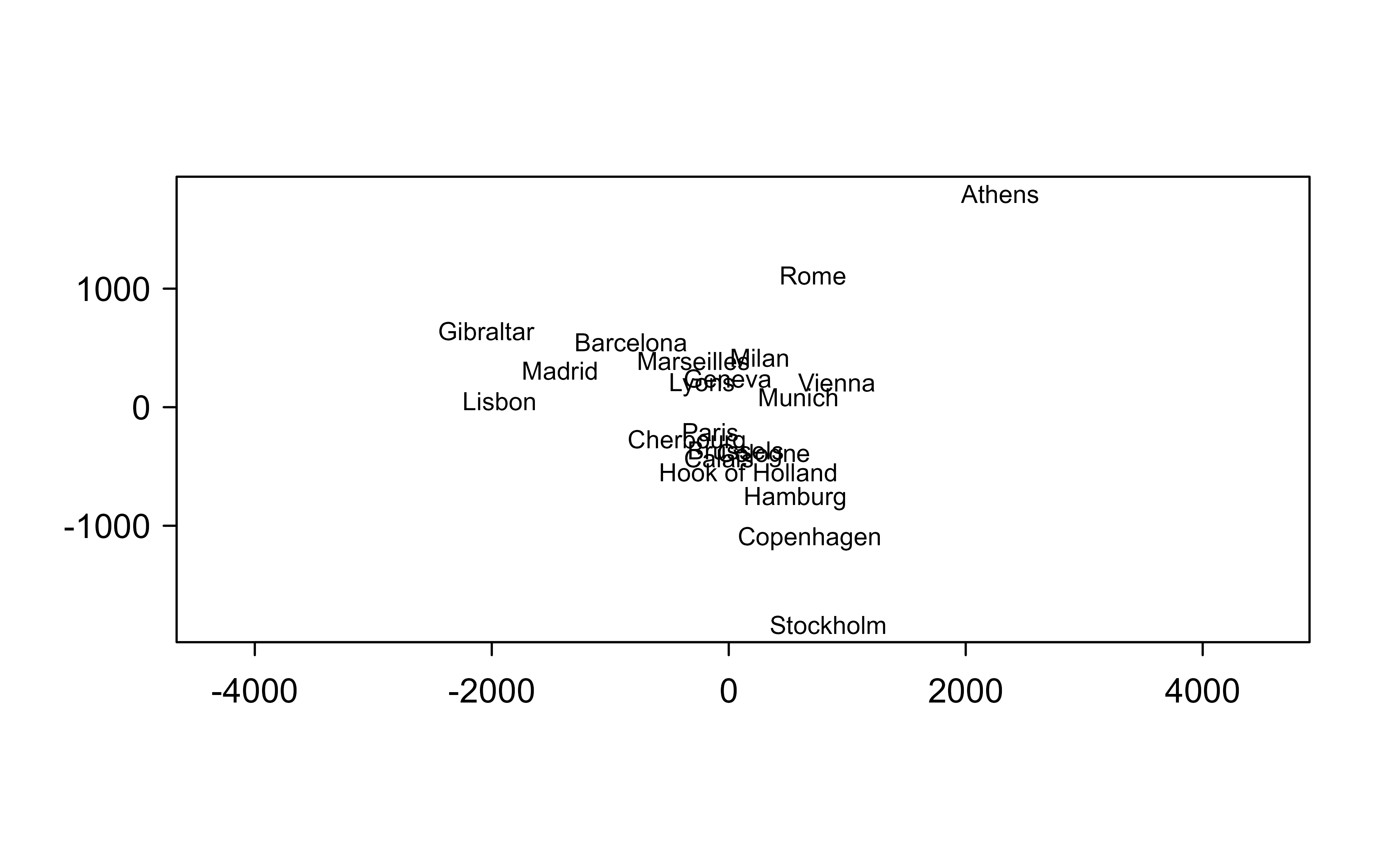
Multidimensional scaling makes a striking promise: hand it only the distances between objects and it reconstructs their coordinates. The cleanest demonstration uses eurodist, the road distances between 21 European cities — no map, no latitudes, just a distance matrix. Classical (metric) MDS factors the double-centered distances and returns a two-dimensional layout:

Show code

mds <- cmdscale(eurodist, k = 2, eig = TRUE)
co  <- mds$points
sum(mds$eig[1:2]) / sum(abs(mds$eig))           # share of structure captured in 2-D
#> [1] 0.7537543
plot(co, type = "n", xlab = "", ylab = "", asp = 1)
text(co, labels = rownames(co), cex = 0.7)

Classical MDS of European road distances. The recovered layout is the map of Europe, up to an arbitrary rotation and reflection.

The picture is the map of Europe — Lisbon and Athens fall at opposite ends, the Scandinavian cities cluster to one side — recovered from distances alone, up to the rotation and reflection that MDS can never pin down (a road map carries no notion of “north”). Metric MDS assumes the distances are quantitatively meaningful. When only their rank order can be trusted (common for perceptual or survey dissimilarities), nonmetric MDS (isoMDS) fits a monotone transform instead and reports stress, the percentage of distance structure it failed to preserve:

Show code

suppressPackageStartupMessages(library(MASS))
nm <- isoMDS(eurodist, k = 2, trace = FALSE)
c(stress_pct = nm$stress, distance_fidelity = cor(dist(co), eurodist))
#>        stress_pct distance_fidelity 
#>         7.5056883         0.9860153

A stress under ~10% and a near-0.99 correlation between recovered and original distances say the two-dimensional embedding is faithful. The workflow generalizes directly: any dissimilarity you can define — between genes, documents, or survey respondents — becomes a low-dimensional map you can actually look at, with stress (or the eigenvalue share) telling you how many dimensions the structure truly needs and how much you sacrificed by stopping at two.

31.3 Nonlinear Multidimensional Scaling

So far the methods have been essentially linear, and classical scaling is literally PCA. But there is interest in nonlinear dimension reduction that preserves not only similarity/dissimilarity, but also other notions of “shape” in the higher dimensional space.

The motivation is a change of assumption. There is sometimes an assumption that the real surface of interest is not in $p$ dimensional space, but it lies on some $d$-dimensional manifold, where $d <<p$. A manifold is a curved surface that looks flat if you zoom in close enough, like the two-dimensional surface of the Earth sitting inside three-dimensional space.

Intuition

Picture a sheet of paper rolled into a Swiss roll. The data are two-dimensional (you could unroll the paper flat), but they sit in three dimensions in a curved way. Straight-line (Euclidean) distance through the roll is misleading: two points on opposite layers are close as the crow flies but far apart along the paper. Nonlinear methods try to measure and preserve distance along the sheet, then flatten it.

This manifold assumption is often true in physical (dynamical) systems, especially when the signal-to-noise ratio is high. Sometimes these nonlinear dimension reduction methods are known as manifold mapping methods. There are many such methods (e.g., kernel PCA) with more being proposed all the time. The four below are among the most influential, and they form a natural progression: ISOMAP fixes the distance measure globally, Local MDS and LLE focus on local structure, and Laplacian Eigenmaps ties the whole idea back to graph theory.

31.3.1 Isometric Feature Mapping

The first method, also known as ISOMAP and developed by Tenenbaum, Silva, and Langford (2000), keeps the familiar machinery of classical scaling but feeds it a smarter notion of distance. Its insight is the Swiss-roll problem above: straight-line distance cheats by cutting through the curved surface, so we should instead measure distance along the manifold.

ISOMAP estimates that along-the-surface distance with a graph, then hands the result to classical MDS. The procedure runs as follows:

For each data point, one finds the neighbors (typically, within some small Euclidean distance). Then, a graph is constructed with an edge between any two neighboring points.
One then approximates the geodesic distance between any two points by the shortest path between points on the graph.⁶
These distances are then collected for all pairs of points and MDS with the classical scaling stress function is applied to the graph distances to get the low-dimensional mapping.

Key idea

ISOMAP is classical MDS with one substitution: replace Euclidean pairwise distances by graph-based geodesic distances. That single change lets a linear method recover nonlinear structure.

31.3.1.1 Why ISOMAP works, and what it costs

The theoretical justification is an asymptotic recovery guarantee. Tenenbaum, Silva, and Langford (2000) (with later convergence proofs by Bernstein and co-authors) show that if the data are sampled from a manifold that is isometric to a convex region of $R^d$ (it can be unrolled without tearing or stretching), and the sampling is dense enough, then the graph shortest-path distance converges to the true geodesic distance as $n \to \infty$. Feeding those geodesics to classical scaling then recovers the underlying flat coordinates up to a rigid motion. The two conditions are exactly the failure modes: a manifold with holes or non-convex boundary (so the flat parameter domain is not convex) breaks the isometry assumption, and short-circuit edges, spurious neighbor links that jump across a fold of the manifold, corrupt every shortest path that uses them, which is why $\epsilon$ or $K$ must be small enough to avoid bridging distinct sheets yet large enough to keep the graph connected.

The computational cost is dominated by the all-pairs shortest paths and the eigendecomposition. With $n$ points, building the neighbor graph is $O(n^2 p)$ naively, all-pairs shortest paths via Dijkstra with a heap is $O(n^2 \log n + n^2 K)$, and the dense classical-scaling eigenproblem is $O(n^3)$. The $O(n^3)$ term and the dense $n \times n$ geodesic matrix make plain ISOMAP impractical beyond a few thousand points; Landmark ISOMAP mitigates this by computing geodesics only from a small set of landmark points and embedding the rest by triangulation.

Like classical scaling, ISOMAP must double-center the squared geodesic distance matrix (apply Equation 31.4 to $\mathbf{D}^{(2)}$ built from geodesics). Because graph geodesics are not exactly Euclidean, the resulting $\mathbf{B}$ typically has some negative eigenvalues; their relative magnitude is a useful diagnostic for how far the data depart from a flat isometric manifold.

31.3.2 Local MDS

Where ISOMAP still tries to honor global distances, the next method gives up on faithfully reproducing distances between far-apart points and instead concentrates on keeping neighbors arranged correctly. Chen and Buja (2009) present a variant of MDS that is more concerned with preserving local similarity/dissimilarity (local MDS) than the global MDS in Section 31.3.1.

They define $\cal{N}$ to be the symmetric set of nearby pairs of points (i.e., a pair $(i,i')$ is in $\cal{N}$ if point $i$ is among the K-nearest neighbors of $i'$, or vice versa). Then, one considers the stress function

\[ S_L (z_1, z_2, \dots, z_n) = \sum_{(i,i') \in \cal{N}} (d_{ii'} - ||z_i - z_{i'}||)^2 + \sum_{(i,i') \notin \cal{N}} w \times (D- ||z_i - z_{i'}||)^2 \]

where $D$ is a large constant and $w$ is a weight. The first sum is ordinary least-squares stress, but applied only to neighbor pairs. The second sum handles non-neighbors: because $w$ is small, points that are not neighbors (i.e., far apart) are given a small weight, so the method barely penalizes getting their distances wrong, and the large target $D$ simply pushes them away from each other.

To simplify, we let $w \sim 1/D$ and let $D \to \infty$, then the stress function becomes

\[ S_L(z_1, z_2, \dots, z_n) = \sum_{(i,i') \in \cal{N}} (d_{ii'} - ||z_i - z_{i'}||)^2 - \tau \sum_{(i,i') \notin \cal{N}} ||z_i - z_{i'}|| \]

where $\tau = 2wD$. Read in two halves: the first term preserves local structure and the second encourages pairs that are non-neighbors to be further apart. The trade-off is governed by two knobs. One implements this by fixing the number of neighbors, $K$, and tuning parameter $\tau$.

Warning

The repulsion term (the one multiplied by $\tau$) is what stops the embedding from collapsing all points onto each other, but set $\tau$ too high and unrelated clusters get pushed apart so aggressively that the local geometry you cared about gets distorted. $K$ and $\tau$ usually need to be tuned together.

31.3.3 Local Linear Embedding

Local MDS preserves local distances. The next method, the LLE procedure of Roweis and Saul (2000), preserves something subtler: the local linear relationships among neighbors. It seeks to preserve the local affine (e.g., same linear combination of a neighbor) structure of the high-dimensional data.

The idea is that each data point is approximated by a linear combination of the neighboring points, and the low-dimensional representation is then constructed to try to preserve this local linear approximation. If point $i$ sits, say, halfway between two of its neighbors in high dimensions, LLE wants it to sit halfway between the images of those same neighbors in the reduced space.

The details, from Hastie, Friedman, and Tibshirani (2001) (Sec. 14.9), come in three steps. First we identify neighborhoods, then we learn the local mixing weights, then we find low-dimensional points that respect those same weights:

For each $x_i$, find the $K$-nearest neighbors $\cal{N}(i)$ in Euclidean distance (where $K <p$).
Approximate each point by the affine mixture of the points in its neighborhood:

\[ \underset{w_{ik}}{\operatorname{min}}||x_i - \sum_{k \in \cal{N}(i)} w_{ik}x_k||^2 \]

with weights $w_{ik}$ such that $w_{ik} = 0, k \notin \cal{N}(i), \sum_{k=1}^n w_{ik} = 1$ (i.e., 0 outside of the neighborhood, and summing to 1 inside of the neighborhood).⁷

31.3.3.0.1 Derivation: the local weights in closed form

Step 2 looks like an unconstrained least-squares problem but the constraint $\sum_k w_{ik} = 1$ is what makes it solvable in closed form. Fix a point $x_i$ with neighbors indexed by $k$. Using $\sum_k w_{ik} = 1$, the reconstruction error can be written entirely in terms of differences from $x_i$,

\[ \Big\| x_i - \sum_{k} w_{ik} x_k \Big\|^2 = \Big\| \sum_{k} w_{ik} (x_i - x_k) \Big\|^2 = \sum_{k,l} w_{ik} w_{il}\, G_{kl}, \tag{31.6}\]

where $G_{kl} = (x_i - x_k)^\top (x_i - x_l)$ is the local Gram matrix of the neighbors measured from $x_i$. Minimizing the quadratic form $w_i^\top \mathbf{G} w_i$ subject to $\mathbf{1}^\top w_i = 1$ is a constrained optimization; the Lagrangian is $w_i^\top \mathbf{G} w_i - \mu(\mathbf{1}^\top w_i - 1)$, and setting the gradient to zero gives $2 \mathbf{G} w_i = \mu \mathbf{1}$, hence

\[ w_i = \frac{\mathbf{G}^{-1}\mathbf{1}}{\mathbf{1}^\top \mathbf{G}^{-1}\mathbf{1}} . \tag{31.7}\]

In practice one solves the linear system $\mathbf{G} w_i = \mathbf{1}$ and rescales, rather than inverting. When $K > p$ (more neighbors than dimensions) $\mathbf{G}$ is singular or ill conditioned, so a ridge term $\mathbf{G} + \delta \mathbf{I}$ with small $\delta$ (regularization proportional to the trace of $\mathbf{G}$) is added; this regularization parameter is, alongside $K$, the main knob in LLE.

We seek points $y_i$ in $d$-dimensional space ($d <p$) to minimize

\[ \sum_{i=1}^n ||y_i - \sum_{k=1}^n w_{ik} y_k||^2 \]

The crucial detail is what is held fixed where: the weights, $w_{ik}$, in step 3 are fixed from step 2. In step 2 we solve for weights with the data fixed; in step 3 we solve for low-dimensional positions with the weights fixed.

We can write the minimization problem in step 3 in matrix notation as the minimization of

\[ \mathbf{tr[(Y - WY)^T (Y - WY)] = tr [Y^T (I - W)^T (I - W)Y]} \]

where $\mathbf{W}$ is $n \times n$ (and known from step 2) and $\mathbf{Y}$ is $n \times d$ for some $d <<p$. It can then be shown that the solution $\hat{\mathbf{Y}}$ is given by the trailing eigenvectors of $\mathbf{M = (I - W)^T(I-W)}$.⁸

31.3.3.0.2 Derivation: why trailing eigenvectors

The objective $\operatorname{tr}[\mathbf{Y}^\top \mathbf{M}\mathbf{Y}]$ with $\mathbf{M} = (\mathbf{I}-\mathbf{W})^\top(\mathbf{I}-\mathbf{W})$ is invariant to translating all $y_i$ by a constant and would be driven to its trivial minimum of zero by collapsing every $y_i$ to one point. Two constraints rule these out: we fix the scale and orientation by requiring $\frac{1}{n}\mathbf{Y}^\top\mathbf{Y} = \mathbf{I}$ (unit covariance, uncorrelated coordinates), and we remove the translational freedom by centering, $\sum_i y_i = \mathbf{0}$. The problem becomes

\[ \min_{\mathbf{Y}} \operatorname{tr}[\mathbf{Y}^\top \mathbf{M}\mathbf{Y}] \quad \text{s.t.} \quad \tfrac{1}{n}\mathbf{Y}^\top\mathbf{Y} = \mathbf{I},\; \mathbf{1}^\top \mathbf{Y} = \mathbf{0}^\top . \tag{31.8}\]

By the Rayleigh-Ritz theorem, the minimizer of a trace of this form under an orthonormality constraint is the set of eigenvectors of $\mathbf{M}$ with the smallest eigenvalues. Now $\mathbf{M}$ is symmetric positive semidefinite, and because each row of $\mathbf{W}$ sums to one, $(\mathbf{I}-\mathbf{W})\mathbf{1} = \mathbf{0}$, so the constant vector $\mathbf{1}$ is an eigenvector of $\mathbf{M}$ with eigenvalue $0$. That eigenvector is exactly the collapsed configuration we excluded with the centering constraint, so we discard it and take the next $d$ eigenvectors, those with the smallest nonzero eigenvalues $\lambda_2 \le \cdots \le \lambda_{d+1}$. This is what “trailing eigenvectors, smallest one discarded” means, and it is the same bottom-of-spectrum structure that reappears in Laplacian Eigenmaps below, the connection Belkin and Niyogi (2003) make precise.

31.3.4 Laplacian Eigenmaps

The last method is close in spirit to Local Linear Embedding but is built explicitly on graph theory, which gives it a clean connection to clustering (Chapter 23). Belkin and Niyogi (2003) proposed Laplacian Eigenmaps (LEs): a nonlinear dimension reduction that preserves local properties and has a natural connection to clustering.

Like the others, LEs make use of a graph that incorporates neighborhood information from the original data. The distinctive ingredient is the graph Laplacian: LE then considers the Laplacian of the graph to preserve local structure in lower dimensions, and in this way it approximates the geometry of the true manifold on which the data arises.

Intuition

The graph Laplacian measures how much a value assigned to each node disagrees with its neighbors’ values, summed over the graph. Finding low-dimensional coordinates that make this disagreement small is exactly asking that connected (nearby) points receive similar coordinates, which is the local-preservation goal restated in the language of graphs.

Suppose we have $n$ $p$-dimensional feature vectors, $\mathbf{x}_{\cal{l}}: \cal{l} = 1, \dots, n$. The procedure constructs a weighted graph with $n$ nodes, one for each vector, and a set of edges connecting neighboring points. The embedding map is then found by computing eigenvectors of the so-called Laplacian. The algorithm, given heuristically below following Belkin and Niyogi (2003), has three steps:

Construct the adjacency graph (i.e., assign an edge between nodes $i$ and $j$ if $\mathbf{x}_i$ is “close” to $\mathbf{x}_j$).
Select the weights; weight the strength of the connection if there is an edge between node $i$ and $j$ (i.e., $W_{ij}$).
Calculate the eigen-decomposition associated with the graph.

We take each step in turn.

Step 1: Adjacency Graph. First we decide which points count as neighbors. There are 2 approaches typically used to decide if two feature vectors (nodes) are “close”:

$\epsilon$-neighborhoods: the $i$th and $j$th nodes are connected if $||\mathbf{x}_i - \mathbf{x}_j|| < \epsilon$, where the norm is usually the Euclidean norm. This approach has the advantage of being geometrically motivated, but it has the disadvantages of sometimes leading to graphs that have disconnected components, and it can be difficult to select $\epsilon$.
$k$ nearest neighbors: the $i$th and $j$th nodes are connected if $i$ is among the $k$ nearest neighbors of $j$ or $j$ is among the $k$ nearest neighbors of $i$. This has the advantage of being simple and does not lead to disconnected graphs, but it is not as “geometrically motivated.”

Step 2: Weight Selection. Next we decide how strongly each edge counts. There are two main approaches:

heat kernel: if the $i$th and $j$th nodes are connected, let

\[ W_{ij} = \exp(-\frac{||\mathbf{x}_i - \mathbf{x}_j||^2}{\theta}) \]

otherwise, let $W_{ij} = 0$. The parameter $\theta$ controls the dependence (weight), so that closer points get larger weights and the influence decays smoothly with distance. This is motivated by the applied math properties of the Laplace-Beltrami operator of differentiable functions on a manifold (Belkin and Niyogi 2003).

binary: let $W_{ij}=1$ if the $i$th and $j$th vertices are connected and 0 if they are not (there is no parameter to choose here).

Step 3: Eigen-decomposition. Finally we read the embedding off the graph’s spectrum. Let $\mathbf{D}$ be a diagonal weight matrix, with elements $D_{ii} = \sum_{j} W_{ij}$ (each node’s total connection strength). Let $\mathbf{L = D - W}$, which is the Laplacian matrix (a symmetric, positive semi-definite matrix) that operates on the vertices of the graph developed in steps 1 and 2.

Consider the eigenvalues and eigenvectors of the generalized eigenvector problem: $\mathbf{Lf} = \lambda \mathbf{Df}$. Specifically, let $\mathbf{f}_0, \dots, \mathbf{f}_{n-1}$ be solutions of this eigen-problem for $0 = \lambda_0 \le \dots \le \lambda_{n-1}$. Note that this is equivalent to finding the eigenvalues of the normalized Laplacian: $\mathbf{D}^{-1/2}\mathbf{L} \mathbf{D}^{-1/2}$ (i.e., $\mathbf{D^{-1/2}L D^{-1/2}f' = \lambda f'}$).

Now, the so-called embedding vector (the lower dimensional presentation of the data) is given by the eigenvectors corresponding to the first (smallest) $m$ eigenvalues $\lambda_1, \dots, \lambda_m$,

\[ \mathbf{x}_i \to (\mathbf{f}_1 (i), \dots, \mathbf{f}_m(i)) \]

31.3.4.0.1 Derivation: the Laplacian quadratic form and the generalized eigenproblem

The reason the Laplacian appears is a one-line identity. For any vector $\mathbf{f} = (f_1, \dots, f_n)^\top$ of coordinates assigned to the nodes (a candidate one-dimensional embedding), the disagreement-with-neighbors objective expands as

\[ \tfrac{1}{2}\sum_{i,j} W_{ij}\,(f_i - f_j)^2 = \sum_i D_{ii} f_i^2 - \sum_{i,j} W_{ij} f_i f_j = \mathbf{f}^\top (\mathbf{D} - \mathbf{W})\,\mathbf{f} = \mathbf{f}^\top \mathbf{L}\,\mathbf{f} . \tag{31.9}\]

The cross term used $\sum_{i,j} W_{ij} f_i^2 = \sum_i D_{ii} f_i^2$ since $D_{ii} = \sum_j W_{ij}$. Equation Equation 31.9 makes the intuition exact: minimizing $\mathbf{f}^\top \mathbf{L}\mathbf{f}$ heavily penalizes giving very different coordinates $f_i, f_j$ to strongly connected ($W_{ij}$ large) points, so connected points are pulled together in the embedding. It also shows $\mathbf{L}$ is positive semidefinite, since the left side is a sum of squares.

To prevent the trivial collapse $\mathbf{f} = \text{const}$ and to fix scale, we impose the constraint $\mathbf{f}^\top \mathbf{D}\,\mathbf{f} = 1$. The $\mathbf{D}$-weighting is deliberate: it normalizes each coordinate by the node’s degree, preventing high-degree hub nodes from dominating and giving the embedding its connection to the normalized cut criterion of spectral clustering (Chapter 23). The Lagrangian is $\mathbf{f}^\top \mathbf{L}\mathbf{f} - \lambda(\mathbf{f}^\top \mathbf{D}\mathbf{f} - 1)$, and its stationarity condition is exactly the generalized eigenproblem stated above,

\[ \mathbf{L}\,\mathbf{f} = \lambda\, \mathbf{D}\,\mathbf{f} . \tag{31.10}\]

The constant vector solves this with $\lambda_0 = 0$ (since $\mathbf{L}\mathbf{1} = \mathbf{0}$), which is the discarded trivial solution; the next $m$ generalized eigenvectors give the embedding. Substituting $\mathbf{g} = \mathbf{D}^{1/2}\mathbf{f}$ turns Equation 31.10 into the standard eigenproblem for the symmetric normalized Laplacian $\mathbf{D}^{-1/2}\mathbf{L}\mathbf{D}^{-1/2}$, which is why the two formulations are equivalent.

Note

We start at $\lambda_1$, not $\lambda_0$. The smallest eigenvalue $\lambda_0 = 0$ corresponds to a constant eigenvector that assigns every point the same coordinate, which carries no information, so it is discarded.

To summarize what LE buys us: one can show through spectral graph theory that these LE embeddings preserve local info in an optimal way (i.e., they are the best locality-preserving mapping). One justification of this procedure is that the Laplacian of a graph is analogous to the Laplace-Beltrami operator on manifolds in differential geometry (i.e., it operates as the divergence of a gradient). It is also the case that the Laplace-Beltrami operator on differentiable functions on a manifold is closely related to the heat flow, which is why we consider the “heat kernel” weights. There is a relatively new area of statistical learning called manifold learning that deals with these issues.

The four methods are more closely related than they first appear. Belkin and Niyogi (2003) discuss the connection between Local Linear Embedding and Laplacian Eigenmaps. In particular, they show that essentially, LLE tries to find the eigenfunctions of the iterated Laplacian $\mathbf{L}^2$ and that these eigenfunctions coincide with those of $\mathbf{L}$, so the two methods are recovering nearly the same structure by different routes.

31.3.5 Practical guidance and the out-of-sample problem

The methods of this section share a small set of decisions that govern whether the embedding is meaningful.

Choosing the neighborhood size. Every local method (ISOMAP, Local MDS, LLE, Laplacian Eigenmaps) hinges on $K$ (or $\epsilon$). Too small and the neighbor graph fragments into disconnected components, so the eigenproblem returns one trivial near-zero eigenvalue per component and the embedding mixes unrelated pieces arbitrarily; too large and edges short-circuit across folds of the manifold, collapsing the nonlinear structure back toward a linear projection. A workable recipe is to pick the smallest $K$ that keeps the graph connected (check the multiplicity of the zero eigenvalue of $\mathbf{L}$, which equals the number of connected components), then increase it modestly for robustness to noise. The heat-kernel bandwidth $\theta$ in Laplacian Eigenmaps is commonly set to a multiple of the median squared neighbor distance.

Choosing the embedding dimension. As with classical scaling, inspect the spectrum. For ISOMAP, plot the residual variance of the classical-scaling reconstruction against $d$ and take the elbow. For the bottom-eigenvalue methods (LLE, Laplacian Eigenmaps), a spectral gap after the $d$-th nonzero eigenvalue suggests an intrinsic dimension of $d$, though such gaps are often soft in real data.

The out-of-sample (Nystrom) extension. The irreversibility noted below has a related but distinct cousin: even forward, these methods embed only the $n$ points used at fit time, with no formula for a new point $x_\ast$. The standard remedy is the Nystrom extension, which treats each embedding coordinate as an eigenfunction of a data-dependent kernel and extends it to $x_\ast$ by a kernel-weighted average over the training points. Bengio and co-authors (2004) show that classical MDS, ISOMAP, LLE, and Laplacian Eigenmaps can all be cast in this common kernel-eigenfunction form, which both unifies the four methods and supplies each with a principled way to embed new observations.

Which method when

Use classical scaling (or PCA) when the structure is plausibly linear and you need reversibility and out-of-sample maps for free. Use ISOMAP when the manifold is a single, convex, well-sampled sheet and global geodesic distances are meaningful. Use LLE or Laplacian Eigenmaps when only local structure is trustworthy, the manifold may be non-convex or have holes, or $n$ is large enough that ISOMAP’s dense $O(n^3)$ geodesic step is prohibitive; their sparse eigenproblems scale far better.

This is only a sampler. There are many different approaches to nonlinear dimension reduction; there is a Matlab toolbox you can download that implements 34 techniques for dimension reduction.

We close with one practical caveat that applies to every nonlinear method in this chapter. One cannot “back project” to the original space with nonlinear dimension reduction methods: if you are given a $z$ above, you cannot say what the associated features in $p$-dimensional space are (i.e., you cannot recover $x$ directly). Linear methods such as PCA can do this, because their mapping is an invertible linear transformation.

Warning

This irreversibility matters in practice. Nonlinear embeddings are excellent for visualization and as inputs to a downstream model, but if your application needs to map a reduced point back to interpretable original features (or to embed brand-new observations not seen during fitting), a linear method like PCA, or a method with an explicit out-of-sample extension, is the safer choice.

This flexibility is the whole point: MDS never needs to see the original coordinates $x_i$, only the pairwise distances $d_{ij}$. So you can run it on data where coordinates do not even exist, such as a panel’s ratings of how similar pairs of items feel.↩︎
The stress function is just a name for the total mismatch between the original distances and the distances in the reduced space. Minimizing stress means making that mismatch as small as possible. Different choices of stress function give the different flavors of MDS below.↩︎
Because every pair contributes a term that couples the positions of two points, there is no closed-form solution; one starts from a random or PCA-based layout and iteratively nudges the points downhill in stress.↩︎
When the distances are Euclidean and the similarity is the centered inner product, classical scaling recovers exactly the same low-dimensional coordinates as principal component analysis. So classical MDS is, in a precise sense, PCA viewed through the lens of pairwise relationships.↩︎
Isotonic regression fits the best monotone (non-decreasing) function to data, which is exactly what we need since $\theta$ is only required to be increasing. Alternating between the two subproblems is a coordinate-descent strategy that steadily lowers the stress.↩︎
The geodesic distance is the length of the shortest path that stays on the manifold, like walking along the surface of the Earth rather than tunneling through it. Short Euclidean hops between near neighbors are trustworthy, so chaining them with a shortest-path algorithm gives a good estimate of the true on-surface distance for far-apart points.↩︎
The constraint that the weights sum to one is what makes the reconstruction affine rather than merely linear, and it gives a useful invariance: the weights do not change if you rotate, rescale, or translate a neighborhood, so they capture only the intrinsic local shape.↩︎
Trailing means the eigenvectors with the smallest eigenvalues (the smallest one is discarded as trivial). Whenever a method ends in an eigenvector computation like this, the layout is found in closed form, with no iterative gradient descent and no local-minimum worries.↩︎

# Multidimensional Scaling and Nonlinear Dimension Reduction {#sec-scaling} ```{r} #| include: false source("_common.R") ``` Imagine you are handed a table of distances between thirty cities, but no map. Could you reconstruct a map from the distances alone? Multidimensional scaling answers yes: given only how far apart things are, it places them as points in a low-dimensional space (say, two dimensions you can plot) so that the plotted distances match the given ones as closely as possible. The same idea works for any data where you can measure how similar or dissimilar pairs of observations are, even when "distance" means something subjective like how alike two products feel to a customer. This chapter introduces two families of methods that share that goal. The first, *multidimensional scaling* (MDS), is a classical, mostly linear approach: it tries to preserve all pairwise distances at once. The second, *nonlinear dimension reduction* (also called *manifold learning*), assumes the data actually live on a curved, lower-dimensional surface sitting inside the high-dimensional space, and tries to "unroll" that surface. By the end you will know what each method optimizes, how the pieces fit together, and when one is preferable to another. These methods complement the linear techniques such as PCA covered in the dimension reduction chapter (@sec-dimension-reduction); here we relax the assumption that the structure we want is a flat subspace. ::: {.callout-important title="Key idea"} All the methods in this chapter take a notion of closeness between observations and find a low-dimensional placement of points that keeps close things close. They differ in *which* closeness they insist on preserving (global vs. local) and in *how flexible* the placement is allowed to be (linear vs. nonlinear). ::: ## Multidimensional Scaling In multidimensional scaling, the main objective is to represent the original observations in a lower-dimensional space such that the "distortion" due to the dimension reduction is minimized. That is, we expect the similarity or dissimilarity between pairs of observations to remain as close as possible after we reduce the dimensionality. We can pursue this goal in two different settings. The first uses actual *metrics*, that is, numerical distances. The second uses only *non-metric* rank orders of the pairwise relationships: for a set of observed similarities or distances between every pair of observations, we seek a presentation of the observations in as few dimensions as possible so that the new proximities nearly match the original proximities, but we ask only that the *ordering* of proximities be respected rather than their exact values. The technique has two historical homes. In classical multivariate statistics, multidimensional scaling is used as a way to visually represent multi-dimensional data, often reducing to two or three dimensions so a human can inspect the result. In modern statistical learning applications, it is often used as a means of presenting observations in lower dimensional spaces for further modeling or analysis, where the reduced coordinates become features fed into a downstream algorithm. Let us set up notation. Consider observations $x_1, \dots, x_n \in R^p$. Let $d_{ij}$ be the distance between observations $i$ and $j$. This distance could be Euclidean distance, $d_{ij} =||x_i - x_j||$, but it can also be more general (e.g., any of the Minkowski distances, or perhaps just some general dissimilarity measure, even a subjective measure of how close the two observations are to each other).^[This flexibility is the whole point: MDS never needs to see the original coordinates $x_i$, only the pairwise distances $d_{ij}$. So you can run it on data where coordinates do not even exist, such as a panel's ratings of how similar pairs of items feel.] So, in multidimensional scaling (MDS), we seek values $z_i, \dots, z_n \in R^k$ ($k <p$) to minimize a stress function.^[The *stress function* is just a name for the total mismatch between the original distances and the distances in the reduced space. Minimizing stress means making that mismatch as small as possible. Different choices of stress function give the different flavors of MDS below.] ::: {.callout-tip title="Intuition"} Think of the $z_i$ as pins you are free to slide around on a corkboard, and the $d_{ii'}$ as target distances printed on a list. The stress function scores how badly your current pin layout violates the target list. MDS slides the pins until the score is as low as it can go. ::: ### Metric Scalings In metric scaling the distances $d_{ii'}$ are genuine numbers we want to reproduce. The three variants below differ only in how they weigh the errors and in whether they work from distances or from similarities. #### Kruskal-Shepard The most direct stress function simply sums the squared gaps between original and reduced distances, $$ S_M(z_1, z_2, \dots, z_n) = \sum_{i \neq i'} (d_{ii'} - ||z_i - z_{i'}||)^2 $$ which is called least squares or Kruskal-Shepard scaling. In words, we want the pairwise distance between the new lower dimensional variables $z_i$ and $z_{i'}$ to be as close as possible to the distance in the original dimension, $d_{ii'}$. This minimization is not analytical but can be solved computationally by a gradient descent algorithm.^[Because every pair contributes a term that couples the positions of two points, there is no closed-form solution; one starts from a random or PCA-based layout and iteratively nudges the points downhill in stress.] The gradient is worth writing out, both because it drives the algorithm and because it exposes the geometry. Differentiating $S_M$ with respect to a single point $z_i$, and using $\partial \|z_i - z_{i'}\| / \partial z_i = (z_i - z_{i'})/\|z_i - z_{i'}\|$, gives $$ \frac{\partial S_M}{\partial z_i} = -4 \sum_{i' \neq i} \big(d_{ii'} - \|z_i - z_{i'}\|\big)\, \frac{z_i - z_{i'}}{\|z_i - z_{i'}\|} . $$ {#eq-scaling-ks-grad} Each term is a spring: the unit vector $(z_i - z_{i'})/\|z_i - z_{i'}\|$ points along the edge, and the scalar $d_{ii'} - \|z_i - z_{i'}\|$ is positive when the points are currently too close (pull apart) and negative when too far (push together). The configuration is in equilibrium when these spring forces balance at every point. A practical consequence of @eq-scaling-ks-grad is the singularity at $z_i = z_{i'}$: coincident points produce an undefined direction, so implementations either perturb ties or, more robustly, use the SMACOF majorization algorithm (Scaling by MAjorizing a COmplicated Function), which replaces the non-smooth stress by a quadratic upper bound at each iteration and so guarantees a monotone, divide-free decrease of stress. #### Sammon Mapping A variation of least squares scaling is the Sammon mapping, which minimizes $$ S_{S_m}(z_1, z_2, \dots, z_n) = \sum_{i \neq i'} \frac{(d_{ii'} - ||z_i - z_{i'}||)^2}{d_{ii'}} $$ The only change from Kruskal-Shepard is the $d_{ii'}$ in the denominator, but it matters: dividing by the original distance makes a fixed error count for more when the pair is close together. As a result the Sammon mapping preserves smaller pairwise distances more-so than larger distances. ::: {.callout-tip title="When to use this"} Reach for the Sammon mapping over plain least squares when the fine-grained structure among nearby points matters more to you than getting the gross, large-scale distances exactly right. ::: #### Classical Scaling A third stress function is called classical scaling, where we start with similarities $s_{ii'}$ rather than distances. Typically, one uses the centered inner product similarity $s_{ii'} = <x_i - \bar{x}, x_{i'} - \bar{x}>$. In this case, we minimize $$ S_C (z_1, \dots, z_n) = \sum_{i \neq i'} (s_{ii'} - <z_i - \bar{z}, z_{i'} - \bar{z}>)^2 $$ Unlike the previous two, this can be solved explicitly in terms of an eigen-decomposition, so no iterative search is needed. In fact, in this context one can show an equivalence between MDS and PCA.^[When the distances are Euclidean and the similarity is the centered inner product, classical scaling recovers exactly the same low-dimensional coordinates as principal component analysis. So classical MDS is, in a precise sense, PCA viewed through the lens of pairwise relationships.] ::: {.callout-note} This equivalence is reassuring but also a limitation. Because classical scaling is PCA in disguise, it can only capture *linear* structure. The nonlinear methods later in the chapter exist precisely to go beyond what an eigen-decomposition of a centered similarity matrix can see. ::: ##### Derivation: from distances to coordinates by double centering The remarkable fact about classical scaling is that we can recover coordinates from distances alone, with no iterative search, provided the distances are Euclidean. Suppose the $d_{ii'}$ arise as Euclidean distances from some unknown centered configuration, $d_{ii'}^2 = \|x_i - x_{i'}\|^2$. Expand the square, $$ d_{ii'}^2 = \|x_i\|^2 + \|x_{i'}\|^2 - 2\, x_i^\top x_{i'} . $$ {#eq-scaling-dsq-expand} Write $b_{ii'} = x_i^\top x_{i'}$ for the (centered) Gram matrix entry. The squared-distance matrix mixes the wanted inner products $b_{ii'}$ with the unwanted diagonal terms $\|x_i\|^2$ and $\|x_{i'}\|^2$. Those unwanted terms are constant along rows and columns, so they can be annihilated by *double centering*: subtract the row mean, the column mean, and add back the grand mean. Define the centering matrix $$ \mathbf{H} = \mathbf{I} - \tfrac{1}{n}\mathbf{1}\mathbf{1}^\top , $$ {#eq-scaling-centering} and let $\mathbf{D}^{(2)}$ be the matrix with entries $d_{ii'}^2$. Applying @eq-scaling-dsq-expand and using $\sum_i x_i = 0$ (the configuration is centered), the row and column means of $\mathbf{D}^{(2)}$ exactly capture the $\|x_i\|^2$ terms, and one obtains the key identity $$ \mathbf{B} = -\tfrac{1}{2}\,\mathbf{H}\,\mathbf{D}^{(2)}\,\mathbf{H} = \mathbf{X}\mathbf{X}^\top , $$ {#eq-scaling-double-center} so that $b_{ii'} = x_i^\top x_{i'}$. The double-centered squared-distance matrix *is* the centered Gram matrix. Since $\mathbf{B}$ is symmetric positive semidefinite of rank at most $p$, take its spectral decomposition $\mathbf{B} = \mathbf{U}\boldsymbol{\Lambda}\mathbf{U}^\top$ with $\lambda_1 \ge \lambda_2 \ge \cdots \ge 0$. The classical-scaling coordinates in $k$ dimensions are the leading scaled eigenvectors, $$ \mathbf{Z} = \mathbf{U}_k \boldsymbol{\Lambda}_k^{1/2}, \qquad z_i = \big(\sqrt{\lambda_1}\,u_{1i}, \dots, \sqrt{\lambda_k}\,u_{ki}\big) . $$ {#eq-scaling-cmds-coords} This is precisely the Eckart-Young optimal rank-$k$ approximation of $\mathbf{B}$, which is why classical scaling minimizes the strain $\|\mathbf{B} - \mathbf{Z}\mathbf{Z}^\top\|_F^2 = \sum_{j>k}\lambda_j^2$ and why dropping the smallest eigenvalues is optimal. Because $\mathbf{B} = \mathbf{X}\mathbf{X}^\top$ shares its nonzero spectrum with the covariance-like matrix $\mathbf{X}^\top\mathbf{X}$, the recovered $z_i$ are exactly the PCA scores, making the MDS/PCA equivalence concrete rather than asserted. ::: {.callout-warning title="When double centering fails"} If the input dissimilarities are not Euclidean (e.g., they violate the triangle inequality, or come from subjective ratings), $\mathbf{B}$ in @eq-scaling-double-center can have negative eigenvalues. Classical scaling then discards them and uses only the positive part, which is the best low-rank Euclidean approximation but is no longer exact. A large negative eigenvalue is a diagnostic that the data are intrinsically non-Euclidean, and a sign that a metric or nonmetric stress method (which never forms $\mathbf{B}$) may fit better. ::: We can verify the two central claims numerically with base R: that double centering the squared-distance matrix recovers the Gram matrix (@eq-scaling-double-center), and that the resulting coordinates coincide with PCA scores up to sign and rotation. ```{r} #| label: cmds-pca-check #| eval: false set.seed(1) X <- scale(matrix(rnorm(20 * 5), 20, 5), center = TRUE, scale = FALSE) D2 <- as.matrix(dist(X))^2 # squared Euclidean distances H <- diag(20) - matrix(1 / 20, 20, 20) # centering matrix B <- -0.5 * H %*% D2 %*% H # double centering # B should equal the centered Gram matrix X X^T: max(abs(B - X %*% t(X))) # classical-scaling coordinates vs PCA scores (first 2 dims): ev <- eigen(B, symmetric = TRUE) Z <- ev$vectors[, 1:2] %*% diag(sqrt(ev$values[1:2])) pcs <- prcomp(X, center = FALSE)$x[, 1:2] # columns match up to sign; compare absolute correlations: round(abs(diag(cor(Z, pcs))), 6) ``` The first number is essentially machine zero (the identity holds exactly), and the correlations are $1$, confirming the MDS/PCA equivalence. ### Nonmetric scalings The metric methods above assume the numbers $d_{ii'}$ are meaningful on a ratio scale. In general, we don't need to have such measures and can apply the procedure to any ordered measure of proximity (e.g., ranks or subjective measures), which is known as nonmetric scalings. Here we trust only the *ranking* of the proximities, not their exact magnitudes, which is exactly right when the data come from human judgments ("A is more like B than like C") rather than physical measurements. For example, Shepard-Kruskal nonmetric scaling minimizes $$ S_{NM} (z_1, z_2, \dots, z_n) = \frac{\sum_{i \neq i'} [||z_i - z_{i'} || - \theta (d_{ii'})]^2}{\sum_{i \neq i'} ||z_i - z_{i'}||^2} $$ for some arbitrary increasing function $\theta$. The function $\theta$ absorbs any monotonic distortion of the scale, so the fit only cares that larger $d_{ii'}$ map to larger reduced distances. One typically doesn't know $\theta$, so we iterate: fix $\theta$ and solve for the $z$'s, then fix the $z$'s and solve for $\theta$, assuming some form for $\theta$ (e.g., isotonic regression).^[Isotonic regression fits the best *monotone* (non-decreasing) function to data, which is exactly what we need since $\theta$ is only required to be increasing. Alternating between the two subproblems is a coordinate-descent strategy that steadily lowers the stress.] ::: {.callout-tip} As with PCA, you usually do not know the target dimension $k$ in advance. In general, we don't know the dimension $k$ to which we want to reduce, so we can fit different solutions and consider the value of the optimized stress function and find the "elbow" as in PCA: the dimension past which adding another axis barely reduces stress. ::: ## Scaling in R: A Worked Example {#sec-scaling-worked} Multidimensional scaling makes a striking promise: hand it only the *distances* between objects and it reconstructs their coordinates. The cleanest demonstration uses `eurodist`, the road distances between 21 European cities --- no map, no latitudes, just a distance matrix. Classical (metric) MDS factors the double-centered distances and returns a two-dimensional layout: ```{r} #| label: mds-classical #| fig-cap: "Classical MDS of European road distances. The recovered layout is the map of Europe, up to an arbitrary rotation and reflection." mds <- cmdscale(eurodist, k = 2, eig = TRUE) co <- mds$points sum(mds$eig[1:2]) / sum(abs(mds$eig)) # share of structure captured in 2-D plot(co, type = "n", xlab = "", ylab = "", asp = 1) text(co, labels = rownames(co), cex = 0.7) ``` The picture *is* the map of Europe --- Lisbon and Athens fall at opposite ends, the Scandinavian cities cluster to one side --- recovered from distances alone, up to the rotation and reflection that MDS can never pin down (a road map carries no notion of "north"). Metric MDS assumes the distances are quantitatively meaningful. When only their *rank order* can be trusted (common for perceptual or survey dissimilarities), nonmetric MDS (`isoMDS`) fits a monotone transform instead and reports **stress**, the percentage of distance structure it failed to preserve: ```{r} #| label: mds-nonmetric suppressPackageStartupMessages(library(MASS)) nm <- isoMDS(eurodist, k = 2, trace = FALSE) c(stress_pct = nm$stress, distance_fidelity = cor(dist(co), eurodist)) ``` A stress under ~10% and a near-0.99 correlation between recovered and original distances say the two-dimensional embedding is faithful. The workflow generalizes directly: any dissimilarity you can define --- between genes, documents, or survey respondents --- becomes a low-dimensional map you can actually look at, with stress (or the eigenvalue share) telling you how many dimensions the structure truly needs and how much you sacrificed by stopping at two. ## Nonlinear Multidimensional Scaling So far the methods have been essentially linear, and classical scaling is literally PCA. But there is interest in nonlinear dimension reduction that preserves not only similarity/dissimilarity, but also other notions of "shape" in the higher dimensional space. The motivation is a change of assumption. There is sometimes an assumption that the real surface of interest is not in $p$ dimensional space, but it lies on some $d$-dimensional manifold, where $d <<p$. A manifold is a curved surface that looks flat if you zoom in close enough, like the two-dimensional surface of the Earth sitting inside three-dimensional space. ::: {.callout-tip title="Intuition"} Picture a sheet of paper rolled into a Swiss roll. The data are two-dimensional (you could unroll the paper flat), but they sit in three dimensions in a curved way. Straight-line (Euclidean) distance through the roll is misleading: two points on opposite layers are close as the crow flies but far apart along the paper. Nonlinear methods try to measure and preserve distance *along the sheet*, then flatten it. ::: This manifold assumption is often true in physical (dynamical) systems, especially when the signal-to-noise ratio is high. Sometimes these nonlinear dimension reduction methods are known as manifold mapping methods. There are many such methods (e.g., kernel PCA) with more being proposed all the time. The four below are among the most influential, and they form a natural progression: ISOMAP fixes the distance measure globally, Local MDS and LLE focus on local structure, and Laplacian Eigenmaps ties the whole idea back to graph theory. ### Isometric Feature Mapping {#sec-isometric-feature-mapping} The first method, also known as ISOMAP and developed by @tenenbaum2000, keeps the familiar machinery of classical scaling but feeds it a smarter notion of distance. Its insight is the Swiss-roll problem above: straight-line distance cheats by cutting through the curved surface, so we should instead measure distance *along* the manifold. ISOMAP estimates that along-the-surface distance with a graph, then hands the result to classical MDS. The procedure runs as follows: - For each data point, one finds the neighbors (typically, within some small Euclidean distance). Then, a graph is constructed with an edge between any two neighboring points. - One then approximates the geodesic distance between any two points by the shortest path between points on the graph.^[The *geodesic* distance is the length of the shortest path that stays on the manifold, like walking along the surface of the Earth rather than tunneling through it. Short Euclidean hops between near neighbors are trustworthy, so chaining them with a shortest-path algorithm gives a good estimate of the true on-surface distance for far-apart points.] - These distances are then collected for all pairs of points and MDS with the classical scaling stress function is applied to the graph distances to get the low-dimensional mapping. ::: {.callout-important title="Key idea"} ISOMAP is classical MDS with one substitution: replace Euclidean pairwise distances by graph-based geodesic distances. That single change lets a linear method recover nonlinear structure. ::: #### Why ISOMAP works, and what it costs The theoretical justification is an asymptotic recovery guarantee. @tenenbaum2000 (with later convergence proofs by Bernstein and co-authors) show that if the data are sampled from a manifold that is *isometric* to a convex region of $R^d$ (it can be unrolled without tearing or stretching), and the sampling is dense enough, then the graph shortest-path distance converges to the true geodesic distance as $n \to \infty$. Feeding those geodesics to classical scaling then recovers the underlying flat coordinates up to a rigid motion. The two conditions are exactly the failure modes: a manifold with holes or non-convex boundary (so the flat parameter domain is not convex) breaks the isometry assumption, and short-circuit edges, spurious neighbor links that jump across a fold of the manifold, corrupt every shortest path that uses them, which is why $\epsilon$ or $K$ must be small enough to avoid bridging distinct sheets yet large enough to keep the graph connected. The computational cost is dominated by the all-pairs shortest paths and the eigendecomposition. With $n$ points, building the neighbor graph is $O(n^2 p)$ naively, all-pairs shortest paths via Dijkstra with a heap is $O(n^2 \log n + n^2 K)$, and the dense classical-scaling eigenproblem is $O(n^3)$. The $O(n^3)$ term and the dense $n \times n$ geodesic matrix make plain ISOMAP impractical beyond a few thousand points; Landmark ISOMAP mitigates this by computing geodesics only from a small set of landmark points and embedding the rest by triangulation. Like classical scaling, ISOMAP must double-center the squared geodesic distance matrix (apply @eq-scaling-double-center to $\mathbf{D}^{(2)}$ built from geodesics). Because graph geodesics are not exactly Euclidean, the resulting $\mathbf{B}$ typically has some negative eigenvalues; their relative magnitude is a useful diagnostic for how far the data depart from a flat isometric manifold. ### Local MDS Where ISOMAP still tries to honor *global* distances, the next method gives up on faithfully reproducing distances between far-apart points and instead concentrates on keeping neighbors arranged correctly. @chen2009 present a variant of MDS that is more concerned with preserving local similarity/dissimilarity (local MDS) than the global MDS in @sec-isometric-feature-mapping. They define $\cal{N}$ to be the symmetric set of nearby pairs of points (i.e., a pair $(i,i')$ is in $\cal{N}$ if point $i$ is among the K-nearest neighbors of $i'$, or vice versa). Then, one considers the stress function $$ S_L (z_1, z_2, \dots, z_n) = \sum_{(i,i') \in \cal{N}} (d_{ii'} - ||z_i - z_{i'}||)^2 + \sum_{(i,i') \notin \cal{N}} w \times (D- ||z_i - z_{i'}||)^2 $$ where $D$ is a large constant and $w$ is a weight. The first sum is ordinary least-squares stress, but applied *only* to neighbor pairs. The second sum handles non-neighbors: because $w$ is small, points that are not neighbors (i.e., far apart) are given a small weight, so the method barely penalizes getting their distances wrong, and the large target $D$ simply pushes them away from each other. To simplify, we let $w \sim 1/D$ and let $D \to \infty$, then the stress function becomes $$ S_L(z_1, z_2, \dots, z_n) = \sum_{(i,i') \in \cal{N}} (d_{ii'} - ||z_i - z_{i'}||)^2 - \tau \sum_{(i,i') \notin \cal{N}} ||z_i - z_{i'}|| $$ where $\tau = 2wD$. Read in two halves: the first term preserves local structure and the second encourages pairs that are non-neighbors to be further apart. The trade-off is governed by two knobs. One implements this by fixing the number of neighbors, $K$, and tuning parameter $\tau$. ::: {.callout-warning} The repulsion term (the one multiplied by $\tau$) is what stops the embedding from collapsing all points onto each other, but set $\tau$ too high and unrelated clusters get pushed apart so aggressively that the local geometry you cared about gets distorted. $K$ and $\tau$ usually need to be tuned together. ::: ### Local Linear Embedding Local MDS preserves local *distances*. The next method, the LLE procedure of @roweis2000, preserves something subtler: the local *linear relationships* among neighbors. It seeks to preserve the local affine (e.g., same linear combination of a neighbor) structure of the high-dimensional data. The idea is that each data point is approximated by a linear combination of the neighboring points, and the low-dimensional representation is then constructed to try to preserve this local linear approximation. If point $i$ sits, say, halfway between two of its neighbors in high dimensions, LLE wants it to sit halfway between the images of those same neighbors in the reduced space. The details, from @hastie2001a (Sec. 14.9), come in three steps. First we identify neighborhoods, then we learn the local mixing weights, then we find low-dimensional points that respect those same weights: 1. For each $x_i$, find the $K$-nearest neighbors $\cal{N}(i)$ in Euclidean distance (where $K <p$). 2. Approximate each point by the affine mixture of the points in its neighborhood: $$ \underset{w_{ik}}{\operatorname{min}}||x_i - \sum_{k \in \cal{N}(i)} w_{ik}x_k||^2 $$ with weights $w_{ik}$ such that $w_{ik} = 0, k \notin \cal{N}(i), \sum_{k=1}^n w_{ik} = 1$ (i.e., 0 outside of the neighborhood, and summing to 1 inside of the neighborhood).^[The constraint that the weights sum to one is what makes the reconstruction *affine* rather than merely linear, and it gives a useful invariance: the weights do not change if you rotate, rescale, or translate a neighborhood, so they capture only the intrinsic local shape.] ##### Derivation: the local weights in closed form Step 2 looks like an unconstrained least-squares problem but the constraint $\sum_k w_{ik} = 1$ is what makes it solvable in closed form. Fix a point $x_i$ with neighbors indexed by $k$. Using $\sum_k w_{ik} = 1$, the reconstruction error can be written entirely in terms of differences from $x_i$, $$ \Big\| x_i - \sum_{k} w_{ik} x_k \Big\|^2 = \Big\| \sum_{k} w_{ik} (x_i - x_k) \Big\|^2 = \sum_{k,l} w_{ik} w_{il}\, G_{kl}, $$ {#eq-scaling-lle-gram} where $G_{kl} = (x_i - x_k)^\top (x_i - x_l)$ is the local Gram matrix of the neighbors measured from $x_i$. Minimizing the quadratic form $w_i^\top \mathbf{G} w_i$ subject to $\mathbf{1}^\top w_i = 1$ is a constrained optimization; the Lagrangian is $w_i^\top \mathbf{G} w_i - \mu(\mathbf{1}^\top w_i - 1)$, and setting the gradient to zero gives $2 \mathbf{G} w_i = \mu \mathbf{1}$, hence $$ w_i = \frac{\mathbf{G}^{-1}\mathbf{1}}{\mathbf{1}^\top \mathbf{G}^{-1}\mathbf{1}} . $$ {#eq-scaling-lle-weights} In practice one solves the linear system $\mathbf{G} w_i = \mathbf{1}$ and rescales, rather than inverting. When $K > p$ (more neighbors than dimensions) $\mathbf{G}$ is singular or ill conditioned, so a ridge term $\mathbf{G} + \delta \mathbf{I}$ with small $\delta$ (regularization proportional to the trace of $\mathbf{G}$) is added; this regularization parameter is, alongside $K$, the main knob in LLE. 3. We seek points $y_i$ in $d$-dimensional space ($d <p$) to minimize $$ \sum_{i=1}^n ||y_i - \sum_{k=1}^n w_{ik} y_k||^2 $$ The crucial detail is what is held fixed where: the weights, $w_{ik}$, in step 3 are fixed from step 2. In step 2 we solve for weights with the data fixed; in step 3 we solve for low-dimensional positions with the weights fixed. We can write the minimization problem in step 3 in matrix notation as the minimization of $$ \mathbf{tr[(Y - WY)^T (Y - WY)] = tr [Y^T (I - W)^T (I - W)Y]} $$ where $\mathbf{W}$ is $n \times n$ (and known from step 2) and $\mathbf{Y}$ is $n \times d$ for some $d <<p$. It can then be shown that the solution $\hat{\mathbf{Y}}$ is given by the trailing eigenvectors of $\mathbf{M = (I - W)^T(I-W)}$.^[*Trailing* means the eigenvectors with the smallest eigenvalues (the smallest one is discarded as trivial). Whenever a method ends in an eigenvector computation like this, the layout is found in closed form, with no iterative gradient descent and no local-minimum worries.] ##### Derivation: why trailing eigenvectors The objective $\operatorname{tr}[\mathbf{Y}^\top \mathbf{M}\mathbf{Y}]$ with $\mathbf{M} = (\mathbf{I}-\mathbf{W})^\top(\mathbf{I}-\mathbf{W})$ is invariant to translating all $y_i$ by a constant and would be driven to its trivial minimum of zero by collapsing every $y_i$ to one point. Two constraints rule these out: we fix the scale and orientation by requiring $\frac{1}{n}\mathbf{Y}^\top\mathbf{Y} = \mathbf{I}$ (unit covariance, uncorrelated coordinates), and we remove the translational freedom by centering, $\sum_i y_i = \mathbf{0}$. The problem becomes $$ \min_{\mathbf{Y}} \operatorname{tr}[\mathbf{Y}^\top \mathbf{M}\mathbf{Y}] \quad \text{s.t.} \quad \tfrac{1}{n}\mathbf{Y}^\top\mathbf{Y} = \mathbf{I},\; \mathbf{1}^\top \mathbf{Y} = \mathbf{0}^\top . $$ {#eq-scaling-lle-embed} By the Rayleigh-Ritz theorem, the minimizer of a trace of this form under an orthonormality constraint is the set of eigenvectors of $\mathbf{M}$ with the *smallest* eigenvalues. Now $\mathbf{M}$ is symmetric positive semidefinite, and because each row of $\mathbf{W}$ sums to one, $(\mathbf{I}-\mathbf{W})\mathbf{1} = \mathbf{0}$, so the constant vector $\mathbf{1}$ is an eigenvector of $\mathbf{M}$ with eigenvalue $0$. That eigenvector is exactly the collapsed configuration we excluded with the centering constraint, so we discard it and take the next $d$ eigenvectors, those with the smallest *nonzero* eigenvalues $\lambda_2 \le \cdots \le \lambda_{d+1}$. This is what "trailing eigenvectors, smallest one discarded" means, and it is the same bottom-of-spectrum structure that reappears in Laplacian Eigenmaps below, the connection @belkin2003 make precise. ### Laplacian Eigenmaps The last method is close in spirit to [Local Linear Embedding] but is built explicitly on graph theory, which gives it a clean connection to clustering (@sec-cluster). @belkin2003 proposed Laplacian Eigenmaps (LEs): a nonlinear dimension reduction that preserves local properties and has a natural connection to clustering. Like the others, LEs make use of a graph that incorporates neighborhood information from the original data. The distinctive ingredient is the *graph Laplacian*: LE then considers the Laplacian of the graph to preserve local structure in lower dimensions, and in this way it approximates the geometry of the true manifold on which the data arises. ::: {.callout-tip title="Intuition"} The graph Laplacian measures how much a value assigned to each node disagrees with its neighbors' values, summed over the graph. Finding low-dimensional coordinates that make this disagreement small is exactly asking that connected (nearby) points receive similar coordinates, which is the local-preservation goal restated in the language of graphs. ::: Suppose we have $n$ $p$-dimensional feature vectors, $\mathbf{x}_{\cal{l}}: \cal{l} = 1, \dots, n$. The procedure constructs a weighted graph with $n$ nodes, one for each vector, and a set of edges connecting neighboring points. The embedding map is then found by computing eigenvectors of the so-called Laplacian. The algorithm, given heuristically below following @belkin2003, has three steps: 1. Construct the adjacency graph (i.e., assign an edge between nodes $i$ and $j$ if $\mathbf{x}_i$ is "close" to $\mathbf{x}_j$). 2. Select the weights; weight the strength of the connection if there is an edge between node $i$ and $j$ (i.e., $W_{ij}$). 3. Calculate the eigen-decomposition associated with the graph. We take each step in turn. Step 1: Adjacency Graph. First we decide which points count as neighbors. There are 2 approaches typically used to decide if two feature vectors (nodes) are "close": 1. $\epsilon$-neighborhoods: the $i$th and $j$th nodes are connected if $||\mathbf{x}_i - \mathbf{x}_j|| < \epsilon$, where the norm is usually the Euclidean norm. This approach has the advantage of being geometrically motivated, but it has the disadvantages of sometimes leading to graphs that have disconnected components, and it can be difficult to select $\epsilon$. 2. $k$ nearest neighbors: the $i$th and $j$th nodes are connected if $i$ is among the $k$ nearest neighbors of $j$ or $j$ is among the $k$ nearest neighbors of $i$. This has the advantage of being simple and does not lead to disconnected graphs, but it is not as "geometrically motivated." Step 2: Weight Selection. Next we decide how strongly each edge counts. There are two main approaches: 1. heat kernel: if the $i$th and $j$th nodes are connected, let $$ W_{ij} = \exp(-\frac{||\mathbf{x}_i - \mathbf{x}_j||^2}{\theta}) $$ otherwise, let $W_{ij} = 0$. The parameter $\theta$ controls the dependence (weight), so that closer points get larger weights and the influence decays smoothly with distance. This is motivated by the applied math properties of the Laplace-Beltrami operator of differentiable functions on a manifold [@belkin2003]. 2. binary: let $W_{ij}=1$ if the $i$th and $j$th vertices are connected and 0 if they are not (there is no parameter to choose here). Step 3: Eigen-decomposition. Finally we read the embedding off the graph's spectrum. Let $\mathbf{D}$ be a diagonal weight matrix, with elements $D_{ii} = \sum_{j} W_{ij}$ (each node's total connection strength). Let $\mathbf{L = D - W}$, which is the Laplacian matrix (a symmetric, positive semi-definite matrix) that operates on the vertices of the graph developed in steps 1 and 2. Consider the eigenvalues and eigenvectors of the generalized eigenvector problem: $\mathbf{Lf} = \lambda \mathbf{Df}$. Specifically, let $\mathbf{f}_0, \dots, \mathbf{f}_{n-1}$ be solutions of this eigen-problem for $0 = \lambda_0 \le \dots \le \lambda_{n-1}$. Note that this is equivalent to finding the eigenvalues of the normalized Laplacian: $\mathbf{D}^{-1/2}\mathbf{L} \mathbf{D}^{-1/2}$ (i.e., $\mathbf{D^{-1/2}L D^{-1/2}f' = \lambda f'}$). Now, the so-called embedding vector (the lower dimensional presentation of the data) is given by the eigenvectors corresponding to the first (smallest) $m$ eigenvalues $\lambda_1, \dots, \lambda_m$, $$ \mathbf{x}_i \to (\mathbf{f}_1 (i), \dots, \mathbf{f}_m(i)) $$ ##### Derivation: the Laplacian quadratic form and the generalized eigenproblem The reason the Laplacian appears is a one-line identity. For any vector $\mathbf{f} = (f_1, \dots, f_n)^\top$ of coordinates assigned to the nodes (a candidate one-dimensional embedding), the disagreement-with-neighbors objective expands as $$ \tfrac{1}{2}\sum_{i,j} W_{ij}\,(f_i - f_j)^2 = \sum_i D_{ii} f_i^2 - \sum_{i,j} W_{ij} f_i f_j = \mathbf{f}^\top (\mathbf{D} - \mathbf{W})\,\mathbf{f} = \mathbf{f}^\top \mathbf{L}\,\mathbf{f} . $$ {#eq-scaling-le-quad} The cross term used $\sum_{i,j} W_{ij} f_i^2 = \sum_i D_{ii} f_i^2$ since $D_{ii} = \sum_j W_{ij}$. Equation @eq-scaling-le-quad makes the intuition exact: minimizing $\mathbf{f}^\top \mathbf{L}\mathbf{f}$ heavily penalizes giving very different coordinates $f_i, f_j$ to strongly connected ($W_{ij}$ large) points, so connected points are pulled together in the embedding. It also shows $\mathbf{L}$ is positive semidefinite, since the left side is a sum of squares. To prevent the trivial collapse $\mathbf{f} = \text{const}$ and to fix scale, we impose the constraint $\mathbf{f}^\top \mathbf{D}\,\mathbf{f} = 1$. The $\mathbf{D}$-weighting is deliberate: it normalizes each coordinate by the node's degree, preventing high-degree hub nodes from dominating and giving the embedding its connection to the normalized cut criterion of spectral clustering (@sec-cluster). The Lagrangian is $\mathbf{f}^\top \mathbf{L}\mathbf{f} - \lambda(\mathbf{f}^\top \mathbf{D}\mathbf{f} - 1)$, and its stationarity condition is exactly the generalized eigenproblem stated above, $$ \mathbf{L}\,\mathbf{f} = \lambda\, \mathbf{D}\,\mathbf{f} . $$ {#eq-scaling-le-geneig} The constant vector solves this with $\lambda_0 = 0$ (since $\mathbf{L}\mathbf{1} = \mathbf{0}$), which is the discarded trivial solution; the next $m$ generalized eigenvectors give the embedding. Substituting $\mathbf{g} = \mathbf{D}^{1/2}\mathbf{f}$ turns @eq-scaling-le-geneig into the standard eigenproblem for the symmetric normalized Laplacian $\mathbf{D}^{-1/2}\mathbf{L}\mathbf{D}^{-1/2}$, which is why the two formulations are equivalent. ::: {.callout-note} We start at $\lambda_1$, not $\lambda_0$. The smallest eigenvalue $\lambda_0 = 0$ corresponds to a constant eigenvector that assigns every point the same coordinate, which carries no information, so it is discarded. ::: To summarize what LE buys us: one can show through spectral graph theory that these LE embeddings preserve local info in an optimal way (i.e., they are the best locality-preserving mapping). One justification of this procedure is that the Laplacian of a graph is analogous to the Laplace-Beltrami operator on manifolds in differential geometry (i.e., it operates as the divergence of a gradient). It is also the case that the Laplace-Beltrami operator on differentiable functions on a manifold is closely related to the heat flow, which is why we consider the "heat kernel" weights. There is a relatively new area of statistical learning called manifold learning that deals with these issues. The four methods are more closely related than they first appear. @belkin2003 discuss the connection between [Local Linear Embedding] and [Laplacian Eigenmaps]. In particular, they show that essentially, LLE tries to find the eigenfunctions of the iterated Laplacian $\mathbf{L}^2$ and that these eigenfunctions coincide with those of $\mathbf{L}$, so the two methods are recovering nearly the same structure by different routes. ### Practical guidance and the out-of-sample problem The methods of this section share a small set of decisions that govern whether the embedding is meaningful. *Choosing the neighborhood size.* Every local method (ISOMAP, Local MDS, LLE, Laplacian Eigenmaps) hinges on $K$ (or $\epsilon$). Too small and the neighbor graph fragments into disconnected components, so the eigenproblem returns one trivial near-zero eigenvalue per component and the embedding mixes unrelated pieces arbitrarily; too large and edges short-circuit across folds of the manifold, collapsing the nonlinear structure back toward a linear projection. A workable recipe is to pick the smallest $K$ that keeps the graph connected (check the multiplicity of the zero eigenvalue of $\mathbf{L}$, which equals the number of connected components), then increase it modestly for robustness to noise. The heat-kernel bandwidth $\theta$ in Laplacian Eigenmaps is commonly set to a multiple of the median squared neighbor distance. *Choosing the embedding dimension.* As with classical scaling, inspect the spectrum. For ISOMAP, plot the residual variance of the classical-scaling reconstruction against $d$ and take the elbow. For the bottom-eigenvalue methods (LLE, Laplacian Eigenmaps), a spectral gap after the $d$-th nonzero eigenvalue suggests an intrinsic dimension of $d$, though such gaps are often soft in real data. *The out-of-sample (Nystrom) extension.* The irreversibility noted below has a related but distinct cousin: even forward, these methods embed only the $n$ points used at fit time, with no formula for a new point $x_\ast$. The standard remedy is the Nystrom extension, which treats each embedding coordinate as an eigenfunction of a data-dependent kernel and extends it to $x_\ast$ by a kernel-weighted average over the training points. Bengio and co-authors (2004) show that classical MDS, ISOMAP, LLE, and Laplacian Eigenmaps can all be cast in this common kernel-eigenfunction form, which both unifies the four methods and supplies each with a principled way to embed new observations. ::: {.callout-tip title="Which method when"} Use classical scaling (or PCA) when the structure is plausibly linear and you need reversibility and out-of-sample maps for free. Use ISOMAP when the manifold is a single, convex, well-sampled sheet and global geodesic distances are meaningful. Use LLE or Laplacian Eigenmaps when only local structure is trustworthy, the manifold may be non-convex or have holes, or $n$ is large enough that ISOMAP's dense $O(n^3)$ geodesic step is prohibitive; their sparse eigenproblems scale far better. ::: This is only a sampler. There are many different approaches to nonlinear dimension reduction; there is a Matlab toolbox you can download that implements 34 techniques for dimension reduction. We close with one practical caveat that applies to every nonlinear method in this chapter. One cannot "back project" to the original space with nonlinear dimension reduction methods: if you are given a $z$ above, you cannot say what the associated features in $p$-dimensional space are (i.e., you cannot recover $x$ directly). Linear methods such as PCA *can* do this, because their mapping is an invertible linear transformation. ::: {.callout-warning} This irreversibility matters in practice. Nonlinear embeddings are excellent for visualization and as inputs to a downstream model, but if your application needs to map a reduced point back to interpretable original features (or to embed brand-new observations not seen during fitting), a linear method like PCA, or a method with an explicit out-of-sample extension, is the safer choice. :::