| Dimension | Public benchmark | Task-specific eval |
|---|---|---|
| Goal | Compare general capability | Measure quality on your task |
| Data source | Public, shared | Your prompts and references |
| Coverage | Broad, generic | Narrow, relevant |
| Leakage risk | High (data may be in pretraining) | Low (private) |
| Predicts production quality | Weak | Strong |
| Maintenance cost | Low (download once) | Higher (curate, refresh) |
| Best use | Shortlist models | Release gate and monitoring |
113 Evaluating LLMs and Guardrails
Once a large language model (LLM) is in a product, the hardest engineering question is no longer “can it generate text” but “is the text good enough, safe enough, and stable enough to ship.” Evaluation answers that question. For a prediction-focused practitioner the situation is familiar: an LLM is a function that maps an input prompt to an output, and we want to estimate the quality of that function on a distribution of inputs we care about. What changes is that the output is free-form text rather than a class label or a number, so the loss function is not handed to us.1 Most of the work in LLM evaluation is the work of defining a usable loss.
Key idea
An LLM is just a function from prompt to text. Evaluation is the problem of inventing a sensible loss for that function, because, unlike classification or regression, no loss comes built in.
This chapter covers where evaluation fits in a modern ML/AI workflow, the difference between generic benchmarks and task-specific evaluation, the common scoring methods (exact match, token overlap, rubric scoring, LLM-as-judge), the quality dimensions that guardrails target (hallucination and faithfulness, toxicity and safety, calibration), and the regression-testing discipline that keeps a prompt or model from silently degrading. The runnable demo is base R: it computes exact-match and token-level \(F_1\) for a question-answering (QA) task and aggregates a scoring rubric over a set of mock model outputs, then prints a scores table and a figure.
113.1 Where Evaluation Fits
A typical LLM application pipeline has a few stages: a base or instruction-tuned model, a prompt template (possibly with retrieved context), optional tool calls, and a set of guardrails that filter or rewrite inputs and outputs. Evaluation sits across all of these. During development you use it to choose a model and tune a prompt. Before release you use it as an acceptance gate. In production you use it as monitoring, sampling live traffic and re-scoring it to detect drift.
The key conceptual move is to treat the whole system, prompt and model and guardrails together, as the object under test. A change to any component can change behavior, so the evaluation set should exercise the system end to end, not just the raw model. This is the same logic as testing a fitted pipeline rather than a single estimator: the thing you deploy is the thing you score.
Intuition
If you score the bare model but ship the model plus a retrieval step plus three guardrails, your number describes something the user never meets. Score the assembled system end to end.
Two failure modes recur. The first is optimizing to a benchmark that does not resemble your traffic, which gives a number that looks good and a product that does not. The second is having no fixed evaluation set at all, so every prompt edit is judged by eyeballing a handful of examples, which does not catch regressions. The rest of the chapter is about avoiding both.
113.2 Benchmarks Versus Task-Specific Evaluation
A benchmark is a fixed, public dataset with a fixed metric, built to compare models on a general capability. Examples include broad knowledge and reasoning suites and coding suites. Benchmarks are useful for model selection and for tracking the field, but they have two limits. They saturate and leak: once a dataset is widely published, later models may have seen it during pretraining, so high scores can reflect memorization rather than capability.2 And they measure a generic skill, not your task. A model that ranks first on a reasoning benchmark can still be wrong about your product’s return policy.
Warning
A leaderboard rank is a shortlisting signal, not a release decision. The model that tops a public benchmark may know nothing about the documents, jargon, and edge cases specific to your product.
Task-specific evaluation is a dataset and metric you build from your own use case: real or realistic prompts, reference answers or rubrics that encode your quality bar, and a metric that reflects the cost of being wrong in your setting. It is smaller and noisier than a benchmark but far more predictive of production quality. The two are complements: use benchmarks to shortlist models, then use a task-specific set to make the final call and to gate releases.
Table 113.1 summarizes the trade-offs.
113.3 Scoring Methods and Their Math
The scoring method is the loss function for text. The right choice depends on how constrained the output is: the more freedom the model has in how it phrases an answer, the softer the metric needs to be. We move from the strictest metric (exact match) to the most flexible (an LLM judge), and the trade is always the same, since flexibility buys you tolerance for paraphrase at the cost of more noise and more bias in the score.
When to use this
Reach for the strictest metric the task allows. A stricter metric is cheaper, more reproducible, and easier to audit. Only loosen it when the output genuinely admits many correct surface forms.
113.3.1 Exact Match
When the correct answer is a short canonical string (a date, a name, a yes/no), exact match (EM) is the simplest metric. Let the model produce prediction \(\hat{y}_i\) for example \(i\) and let \(y_i\) be the reference. After a normalization function \(g(\cdot)\) that lowercases, strips punctuation, and trims whitespace,
\[ \mathrm{EM} = \frac{1}{n} \sum_{i=1}^{n} \mathbb{1}\!\left[\, g(\hat{y}_i) = g(y_i) \,\right], \]
where \(\mathbb{1}[\cdot]\) is the indicator function and \(n\) is the number of examples. EM is strict: “Paris” and “Paris, France” both differ from “the city of Paris,” so EM understates quality when answers are phrased loosely. It is the right metric only when there is a single accepted surface form.
113.3.2 Token-Level F1
For short free-form answers, a softer metric compares the bag of tokens. Treat the prediction and reference as multisets of tokens after normalization. Let \(\mathrm{TP}\) be the number of shared tokens (counted with multiplicity), so that
\[ \text{precision} = \frac{\mathrm{TP}}{|\hat{y}|}, \qquad \text{recall} = \frac{\mathrm{TP}}{|y|}, \]
where \(|\hat{y}|\) and \(|y|\) are the token counts of the prediction and reference. The \(F_1\) score is their harmonic mean,
\[ F_1 = \frac{2 \cdot \text{precision} \cdot \text{recall}}{\text{precision} + \text{recall}}, \]
with \(F_1 = 0\) when there are no shared tokens. This is the standard metric for extractive QA datasets. It rewards partial overlap, so “Paris France” against the reference “Paris” earns precision \(1/2\) and recall \(1\), giving \(F_1 = 2/3\) rather than zero. The number of shared tokens uses multiset intersection, so a token that appears twice in the reference but once in the prediction contributes one to \(\mathrm{TP}\).3
113.3.3 Rubric Scoring
When the output is a paragraph, a single string match is meaningless. A rubric breaks quality into named criteria, each scored on an ordinal scale, and combines them with weights. For example \(i\) with criteria \(j = 1, \dots, K\), let \(s_{ij}\) be the score on criterion \(j\) (say \(0\) to \(1\)) and \(w_j \ge 0\) a weight with \(\sum_j w_j = 1\). The aggregate score for example \(i\) is
\[ S_i = \sum_{j=1}^{K} w_j \, s_{ij}, \]
and the dataset score is the mean \(\bar S = \frac{1}{n}\sum_{i=1}^n S_i\). Rubrics make the quality definition explicit and auditable, which matters when several people disagree about what “good” means. The scores \(s_{ij}\) can come from human raters or from an LLM judge.
Tip
Writing the rubric is itself the most valuable step. Forcing yourself to name the criteria and assign weights surfaces hidden disagreements about quality before they turn into arguments over a single output.
113.3.4 LLM-as-Judge
Asking a strong LLM to grade another model’s output is LLM-as-judge. It scales to free-form text where references are unavailable, and it can apply a rubric written in natural language. It is also biased and noisy, so treat the judge as a measurement instrument that itself needs validation against human labels. Known biases include position bias (preferring the first option in a pairwise comparison), length bias (preferring longer answers), and self-preference (favoring outputs from the same model family). Mitigations include randomizing option order, calibrating against a human-labeled subset, and reporting agreement rates rather than treating the judge as ground truth.
Warning
A judge that grades its own model’s outputs can flatter them. Never let a model be the sole arbiter of its own release without first checking how well it agrees with human raters.
Table 113.2 compares the methods.
| Method | Output type | Needs reference | Cost | Main weakness |
|---|---|---|---|---|
| Exact match | Canonical string | Yes | Trivial | Too strict |
| Token F1 | Short answer | Yes | Trivial | Ignores meaning/order |
| Rubric (human) | Free-form text | Optional | High | Slow, rater drift |
| Rubric (LLM judge) | Free-form text | Optional | Low | Judge bias |
| Pairwise (LLM judge) | Free-form text | No | Low | Judge bias |
113.4 Guardrail Dimensions
So far the metrics ask “is the answer right.” Guardrails ask a different family of questions: “is the answer supported, is it safe, and does it know what it does not know.” Guardrails are the checks and filters that keep a system within acceptable behavior, and each one maps to a measurable evaluation dimension. We take three in turn: faithfulness, safety, and calibration.
113.4.1 Hallucination and Faithfulness
A hallucination is a confident statement not supported by the input or by fact. In retrieval-augmented settings (Chapter 111) the precise target is faithfulness: every claim in the output should be entailed by the provided context. If a response decomposes into claims \(c_1, \dots, c_m\) and \(e_k \in \{0,1\}\) marks whether claim \(k\) is supported by the context, a faithfulness score is
\[ \text{faithfulness} = \frac{1}{m}\sum_{k=1}^{m} e_k. \]
The entailment labels \(e_k\) come from a natural-language-inference model or an LLM judge. Faithfulness is distinct from correctness: an answer can be faithful to a wrong document, or correct but unsupported by the retrieved context. Report both when you can.
Note
Faithfulness measures the link between the output and the context you gave the model, not the link between the output and the truth. A faithful answer grounded in a wrong document is still wrong, which is why correctness and faithfulness are reported as separate numbers.
113.4.2 Toxicity and Safety
Safety evaluation measures the rate at which a system produces disallowed content (harassment, dangerous instructions, leaked secrets) and the rate at which it incorrectly refuses benign requests. These are two error types. With a held-out set of adversarial prompts and benign prompts, you estimate a violation rate on the adversarial set and an over-refusal rate on the benign set.4 Pushing one to zero usually raises the other, so safety tuning is an operating-point choice, the same trade-off as a classification threshold.
Intuition
Safety has two error types pulling against each other: letting bad content through, and blocking good content. Driving the violation rate to zero by refusing more aggressively just trades one failure for the other. The goal is a deliberate operating point, not a corner.
113.4.3 Calibration
A model is calibrated if its stated confidence matches its accuracy, the same property studied in the probability calibration chapter (Chapter 86). If the model (or a wrapper) emits a probability \(\hat p\) that its answer is correct, calibration asks whether, among all answers with \(\hat p \approx 0.8\), about 80 percent are in fact correct.
Intuition
Calibration is about honesty, not accuracy. A weather forecaster who says “70 percent chance of rain” is well calibrated if it rains on about 70 percent of such days, even if she is wrong half the time. A model can be accurate but overconfident, or mediocre but well calibrated.
Bin the predictions into \(B\) confidence bins. For bin \(b\) with index set \(I_b\), let
\[ \text{acc}(b) = \frac{1}{|I_b|}\sum_{i \in I_b} \mathbb{1}[\hat y_i = y_i], \qquad \text{conf}(b) = \frac{1}{|I_b|}\sum_{i \in I_b} \hat p_i . \]
The expected calibration error aggregates the gap, weighting each bin by its share of examples:
\[ \mathrm{ECE} = \sum_{b=1}^{B} \frac{|I_b|}{n}\,\bigl|\,\text{acc}(b) - \text{conf}(b)\,\bigr|. \]
A low \(\mathrm{ECE}\) means confidence is trustworthy, which lets you route low-confidence answers to a human or a fallback. Calibration matters for guardrails because an abstention policy (“answer only when confident”) is only as good as the confidence estimate behind it. When you need distribution-free guarantees on such abstention decisions, conformal prediction (Chapter 85) supplies confidence sets with finite-sample coverage.
113.5 Regression Testing for Prompts
A prompt is code.5 A small wording change, a new model version, or a tweaked system message can shift behavior in ways that are invisible until a user hits them. Regression testing treats the evaluation set as a test suite: pin a set of inputs with expected properties, run the current system against it on every change, and compare to the last accepted run. A change is accepted only if the aggregate score does not drop and no protected example regresses.
Practical structure: keep golden examples (inputs with reference answers or must-pass assertions) under version control, run them in continuous integration, and fail the build when the score falls below a threshold or when any example flagged as critical flips from pass to fail. Track scores over time so you can see slow drift, not just single-commit breaks. Because LLM outputs can be nondeterministic, fix the sampling temperature to zero for tests where you can, and for the rest run several samples and compare distributions rather than single outputs.
Tip
A single passing example is weak evidence when the model samples randomly. For nondeterministic tests, run each input several times and assert on the distribution (for example, the answer must pass in at least 9 of 10 draws) rather than on one lucky output.
113.6 Runnable Demo: EM, Token F1, and Rubric Aggregation
The following base R code implements the QA metrics and rubric aggregation from the math above, runs them over a small set of mock model outputs, and reports a scores table and a figure. It uses only base R so it runs anywhere.
Show code
# Normalization shared by exact match and token F1: lowercase, drop
# punctuation, collapse and trim whitespace. This mirrors standard QA
# evaluation so that "Paris." and "paris" compare equal.
normalize_text <- function(x) {
  x <- tolower(x)
  x <- gsub("[[:punct:]]", " ", x)
  x <- gsub("\\s+", " ", x)
  trimws(x)
}

tokenize <- function(x) {
  x <- normalize_text(x)
  if (nchar(x) == 0) return(character(0))
  strsplit(x, " ", fixed = TRUE)[[1]]
}

exact_match <- function(pred, ref) {
  as.integer(normalize_text(pred) == normalize_text(ref))
}

# Token-level F1 using multiset (bag-of-tokens) intersection.
token_f1 <- function(pred, ref) {
  p_tok <- tokenize(pred)
  r_tok <- tokenize(ref)
  if (length(p_tok) == 0 && length(r_tok) == 0) return(1)
  if (length(p_tok) == 0 || length(r_tok) == 0) return(0)

  p_counts <- table(p_tok)
  r_counts <- table(r_tok)
  shared   <- intersect(names(p_counts), names(r_counts))
  # multiset intersection: min count per shared token
  tp <- sum(pmin(p_counts[shared], r_counts[shared]))
  if (tp == 0) return(0)

  precision <- tp / length(p_tok)
  recall    <- tp / length(r_tok)
  2 * precision * recall / (precision + recall)
}
Show code
# Mock QA outputs: a model's predictions against gold references.
qa <- data.frame(
  question = c(
    "What is the capital of France?",
    "Who wrote Pride and Prejudice?",
    "What year did the first moon landing occur?",
    "What is the chemical symbol for sodium?",
    "How many continents are there?"
  ),
  reference = c("Paris", "Jane Austen", "1969", "Na", "seven"),
  prediction = c(
    "Paris, France",          # partial overlap, not exact
    "Jane Austen",            # exact
    "It happened in 1969.",   # contains the answer plus extra tokens
    "Sodium",                 # wrong surface form
    "7"                       # correct concept, different token
  ),
  stringsAsFactors = FALSE
)

qa$EM <- mapply(exact_match, qa$prediction, qa$reference)
qa$F1 <- round(mapply(token_f1, qa$prediction, qa$reference), 3)
qa
#>                                      question   reference           prediction
#> 1              What is the capital of France?       Paris        Paris, France
#> 2              Who wrote Pride and Prejudice? Jane Austen          Jane Austen
#> 3 What year did the first moon landing occur?        1969 It happened in 1969.
#> 4     What is the chemical symbol for sodium?          Na               Sodium
#> 5              How many continents are there?       seven                    7
#>   EM    F1
#> 1  0 0.667
#> 2  1 1.000
#> 3  0 0.400
#> 4  0 0.000
#> 5  0 0.000
Show code
| metric | score |
|---|---|
| Exact match | 0.200 |
| Token F1 | 0.413 |
Table 113.3 reports the aggregate scores. The gap between EM and \(F_1\) is the point: EM credits only the second example, while \(F_1\) gives partial credit to “Paris, France” and to the answer embedded in a longer sentence. Neither metric handles “7” versus “seven,” which is a reminder that surface-form metrics miss meaning and why semantic or judge-based scoring is sometimes needed.
Now the rubric. We score four free-form summaries on three weighted criteria.
Show code
# Rubric scores in [0,1] for three criteria, assigned here as mock
# judge or human ratings for four candidate summaries.
rubric_scores <- data.frame(
  output      = paste0("summary_", 1:4),
  relevance   = c(0.9, 0.6, 1.0, 0.4),
  faithfulness= c(1.0, 0.5, 0.8, 0.3),
  fluency     = c(0.8, 0.9, 0.7, 0.6),
  stringsAsFactors = FALSE
)

# Weights encode the quality bar: faithfulness matters most here.
weights <- c(relevance = 0.3, faithfulness = 0.5, fluency = 0.2)
stopifnot(abs(sum(weights) - 1) < 1e-8)

crit_mat <- as.matrix(rubric_scores[, names(weights)])
rubric_scores$aggregate <- round(as.numeric(crit_mat %*% weights), 3)
rubric_scores
#>      output relevance faithfulness fluency aggregate
#> 1 summary_1       0.9          1.0     0.8      0.93
#> 2 summary_2       0.6          0.5     0.9      0.61
#> 3 summary_3       1.0          0.8     0.7      0.84
#> 4 summary_4       0.4          0.3     0.6      0.39
Show code
rubric_summary <- data.frame(
  statistic = c("Mean aggregate", "Min aggregate", "Max aggregate"),
  value     = round(c(mean(rubric_scores$aggregate),
                      min(rubric_scores$aggregate),
                      max(rubric_scores$aggregate)), 3)
)
knitr::kable(rubric_summary,
caption = "Weighted rubric aggregate across four mock outputs.")| statistic | value |
|---|---|
| Mean aggregate | 0.693 |
| Min aggregate | 0.390 |
| Max aggregate | 0.930 |
Table 113.4 summarizes the spread of the weighted aggregate across the four mock outputs.
Show code
op <- par(mar = c(5, 4, 3, 1))
bp <- barplot(
  height    = rubric_scores$aggregate,
  names.arg = rubric_scores$output,
  ylim      = c(0, 1),
  col       = ifelse(rubric_scores$aggregate >= 0.7, "steelblue", "grey70"),
  ylab      = "weighted aggregate score",
  main      = "Rubric aggregate by candidate output"
)
abline(h = 0.7, lty = 2, lwd = 2, col = "firebrick")
text(bp, rubric_scores$aggregate + 0.04, labels = rubric_scores$aggregate)
par(op)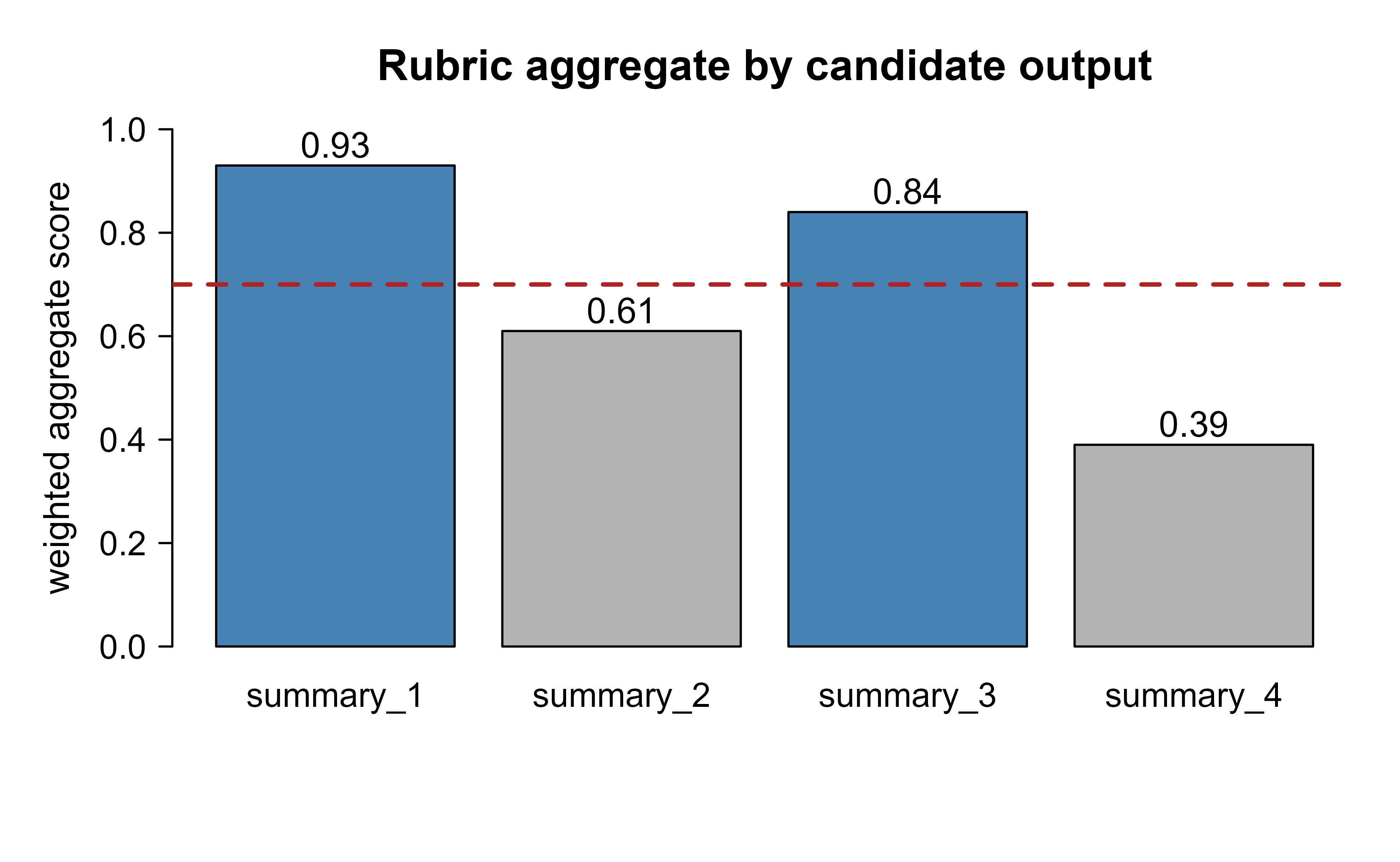
Figure 113.1 shows the release gate in action: with a threshold of \(0.7\) on the weighted aggregate, two of the four mock summaries pass. Lowering faithfulness weight would let the unfaithful summary through, which is exactly the kind of policy choice a rubric makes explicit.
113.7 A Production-Style Judge Call (Not Run Here)
The metrics above need no external service. An LLM-as-judge does. The chunk below shows current, idiomatic R for calling a judge through the ellmer package and parsing a structured score. It is marked eval = FALSE because ellmer is not installed in this build and a live call needs an API key.
Show code
library(ellmer)

# A judge that returns a structured rubric score for one answer.
judge <- chat_anthropic(
  model  = "claude-sonnet-4-5",
  system_prompt = paste(
    "You are a strict grader. Score the ANSWER against the QUESTION and",
    "CONTEXT on three criteria, each from 0 to 1: relevance, faithfulness",
    "(every claim supported by CONTEXT), and fluency."
  )
)

score_type <- type_object(
  relevance    = type_number("Relevance to the question, 0 to 1."),
  faithfulness = type_number("Support by the context, 0 to 1."),
  fluency      = type_number("Readability, 0 to 1."),
  rationale    = type_string("One sentence explaining the scores.")
)

grade_one <- function(question, context, answer) {
  prompt <- sprintf(
    "QUESTION:\n%s\n\nCONTEXT:\n%s\n\nANSWER:\n%s",
    question, context, answer
  )
  judge$chat_structured(prompt, type = score_type)
}

# To reduce position and length bias, randomize option order in pairwise
# comparisons and validate the judge against a human-labeled subset before
# trusting its scores in a release gate.
The same structured output then flows into the weighted aggregation from the runnable demo: collect relevance, faithfulness, and fluency, multiply by the weight vector, and compare the mean to the release threshold.
113.8 Practical Guidance and Pitfalls
Build the task-specific set first. A few hundred curated examples that look like your traffic beat any public benchmark for deciding whether to ship. Stratify the set by the slices you care about (topic, user type, difficulty) and report scores per slice, because an aggregate can hide a regression in a minority slice.
Match the metric to the output. Use EM only for canonical short answers, token \(F_1\) for short free-form answers, rubrics for paragraphs, and a judge only after you have measured its agreement with humans. Reporting a single headline number across mixed output types hides more than it reveals.
Treat the judge as an instrument, not an oracle. Calibrate it against a human-labeled subset, randomize option order, watch for length and self-preference bias, and report inter-rater agreement (for example Cohen’s \(\kappa\)) between judge and humans. If the judge disagrees with humans more than humans disagree with each other, the judge is not ready to gate releases.
Separate correctness from faithfulness from safety. They fail independently. A RAG system can be faithful to a wrong document, correct from memory but unsupported, or safe yet useless. Score each dimension on its own and decide the operating point deliberately, since reducing over-refusal usually raises the violation rate.
Pin the evaluation set and version it. Refresh it on a schedule, not on a whim, and keep a frozen subset so historical scores stay comparable. Fix sampling temperature to zero in tests where you can, and for nondeterministic cases compare score distributions over several samples rather than single outputs.
When to use this
Build a full evaluation harness once a change can reach users, once several people must agree on what “good” means, or once you need to detect drift over time. Throwaway prototypes and exploratory prompting do not need one; a small golden set and a couple of assertions are enough.
When not to do heavy evaluation: throwaway prototypes and exploratory prompting do not need a full harness. The cost is justified once a change can reach users, once several people must agree on quality, or once you need to detect drift over time. Below that bar, a small golden set and a couple of assertions are enough.
To summarize the workflow: shortlist models with public benchmarks, then build a private task-specific set that looks like your traffic; pick the strictest scoring method the output allows, and validate any LLM judge against humans before trusting it; score correctness, faithfulness, and safety as separate dimensions and choose the operating point on purpose; and finally pin the set, run it on every change, and watch the scores over time so that drift shows up as a trend rather than a surprise.
113.9 Further Reading
- Rajpurkar, Zhang, Lopyrev, and Liang (2016) introduced SQuAD and the token-level exact-match and \(F_1\) metrics used for extractive QA.
- Lin (2004) defined ROUGE, the recall-oriented overlap metric for summarization.
- Papineni, Roukos, Ward, and Zhu (2002) defined BLEU, the precision-oriented n-gram overlap metric for generation.
- Zheng, Chiang, Sheng, and colleagues (2023) studied LLM-as-judge, documenting position, length, and self-preference biases and agreement with human raters.
- Guo, Pleiss, Sun, and Weinberger (2017) analyzed calibration of modern neural networks and the expected calibration error.
- Naeini, Cooper, and Hauskrecht (2015) introduced the binned estimator behind the expected calibration error.
- Es, James, Espinosa-Anke, and Schockaert (2024) proposed RAGAS, a framework for faithfulness and answer-relevance scoring in retrieval-augmented generation.
- Liang, Bommasani, and colleagues (2022) presented HELM, a holistic benchmarking framework emphasizing multiple metrics and scenarios over a single score.
For a classifier the loss is obvious: did the predicted label match the true label. For free-form text there is no single “true” string, since many wordings can be equally good and many can be equally bad, so we have to construct a scoring rule before we can measure anything.↩︎
This is the text analogue of testing a model on its own training data. If the answers were in the pretraining corpus, a high benchmark score measures recall of seen examples, not the generalization you actually care about.↩︎
The multiset (bag of tokens with counts) keeps the metric honest about repetition: a prediction that repeats a correct word ten times does not earn ten times the credit. It also means token \(F_1\) ignores word order, so “dog bites man” and “man bites dog” score identically, which is one of its known blind spots.↩︎
An over-refusal is the safety analogue of a false positive: the system flags a harmless request as dangerous and declines it. Track it explicitly, because a model that refuses everything is perfectly “safe” and completely useless.↩︎
Treat it that way literally: keep prompts in version control, review changes, and never edit the production prompt without running it past the evaluation set first. A one-word change to a system message is a deploy.↩︎