56  Federated Learning

Picture a consortium of three hospitals that each want a better model for predicting which patients will be readmitted within thirty days. Each hospital alone has only a few thousand records, too few to train a model that generalizes. Pooling the records into one database would solve the statistical problem instantly, but it is a non-starter: patient records cannot leave the building, regulators forbid it, and even if they did not, no hospital wants to hand a competitor its raw data. The data is locked in place, yet the value lives in the combination.

Federated learning is the answer to exactly this tension. Instead of moving data to a central model, it moves the model to the data. A coordinating server holds a shared model, ships a copy to each participant (each client), and asks every client to train on its own private data for a little while. The clients send back not their data but their updated model parameters. The server averages those updates into a new shared model and repeats. Over many such rounds the shared model improves as if it had seen all the data, while every raw record stays where it started. The phrase to keep in mind is that data stays put and only models travel.

This pattern matters far beyond hospitals. It is how a phone keyboard learns the words you type without your messages ever leaving the device, how banks build fraud models across institutions that legally cannot share transactions, and how manufacturers pool sensor data across factories that sit behind separate firewalls. Wherever data is abundant but trapped by privacy, regulation, ownership, or sheer bandwidth, federated learning offers a way to learn from all of it at once.

The chapter builds the idea from the ground up. We start with the optimization problem federated learning actually solves, derive the FedAvg algorithm that almost everyone uses, and then confront the two facts that make the field hard in practice: communication is expensive, and the clients’ data is not identically distributed. We close with privacy and security, since the whole point was to protect data, and a runnable base-R simulation that trains a logistic model across several clients and shows the global loss falling round by round, compared head to head against ordinary centralized training.

Note

This chapter assumes comfort with gradient descent and with the idea of minimizing an average loss over a dataset. The running example is logistic regression because its loss is convex and easy to reason about, but nothing about the federated machinery is specific to that choice; the same recipe wraps around neural networks (Chapter 15), gradient-boosted trees (Chapter 12), and more.

56.1 The federated optimization problem

Write the model parameters as a vector \(w \in \mathbb{R}^d\). There are \(K\) clients. Client \(k\) holds a private dataset \(\mathcal{D}_k\) with \(n_k\) examples, and the total number of examples across all clients is \(n = \sum_{k=1}^{K} n_k\). On its own data, client \(k\) has a local objective, the average loss over its examples,

\[ F_k(w) \;=\; \frac{1}{n_k} \sum_{i \in \mathcal{D}_k} \ell\bigl(w; x_i, y_i\bigr), \]

where \(\ell\) is the per-example loss (for logistic regression, the negative log-likelihood of one labeled point). The quantity we would like to minimize is the loss we would get if all the data were pooled. Because pooling just concatenates the datasets, that global objective is a weighted average of the local ones, weighted by how much data each client holds:

\[ F(w) \;=\; \sum_{k=1}^{K} \frac{n_k}{n}\, F_k(w) \;=\; \frac{1}{n}\sum_{k=1}^{K} \sum_{i \in \mathcal{D}_k} \ell\bigl(w; x_i, y_i\bigr). \]

The goal is the same \(w^\star = \arg\min_w F(w)\) you would compute centrally. The constraint is what is new: the server may never see any \(x_i\) or \(y_i\). It can only send \(w\) to clients and receive things computed from \(w\) and the local data, such as gradients or updated parameters.

Key idea

The federated objective \(F(w)\) is identical to the centralized objective. Federated learning is not a different model or a different loss. It is a constrained way of optimizing the same loss, where the optimizer is forbidden from gathering the data in one place.

This framing immediately suggests a naive algorithm. Each client computes the gradient of its local objective at the current \(w\), the server averages those gradients (weighting by \(n_k/n\)), takes one gradient-descent step, and broadcasts the new \(w\). Because the gradient of \(F\) is the weighted average of the gradients of the \(F_k\),

\[ \nabla F(w) \;=\; \sum_{k=1}^{K} \frac{n_k}{n}\, \nabla F_k(w), \]

this federated gradient descent is mathematically identical to running gradient descent on the pooled data. It is correct but wasteful: it spends one full round of communication, the slow and expensive part, to make one tiny gradient step. Real networks have latency and limited bandwidth, and a phone on a cellular connection is not going to exchange messages a million times. The central problem of federated learning is to extract more progress from each expensive round of communication. That is what FedAvg does.

56.1.1 Why the federated gradient decomposes

The identity \(\nabla F(w) = \sum_k (n_k/n)\nabla F_k(w)\) is the algebraic backbone of every aggregation rule in this chapter, so it is worth seeing it fall out of the definitions rather than asserting it. Gradients are linear operators, and \(F\) is a finite weighted sum of the \(F_k\), so

\[ \nabla F(w) = \nabla\!\left[\frac{1}{n}\sum_{k=1}^{K}\sum_{i\in\mathcal{D}_k}\ell(w;x_i,y_i)\right] = \frac{1}{n}\sum_{k=1}^{K}\sum_{i\in\mathcal{D}_k}\nabla_w\,\ell(w;x_i,y_i) = \sum_{k=1}^{K}\frac{n_k}{n}\,\nabla F_k(w), \]

where the last step pulls \(1/n = (n_k/n)\cdot(1/n_k)\) out of each inner sum and recognizes \(\frac{1}{n_k}\sum_{i\in\mathcal{D}_k}\nabla\ell = \nabla F_k(w)\). The same weights \(n_k/n\) appear in the server’s average precisely because they are the weights that make the local objectives reconstruct the global one. This also pins down the unbiasedness statement of Section 56.4: for a fixed client \(k\), the local gradient \(\nabla F_k(w)\) is an unbiased estimate of the global gradient \(\nabla F(w)\) only when each client’s data is drawn from the same distribution, i.e. \(\nabla F_k(w) = \nabla F(w)\) for every \(k\), which is exactly the IID assumption. (Averaging over a client sampled with probability \(n_k/n\) is unbiased unconditionally, since \(\sum_k (n_k/n)\nabla F_k(w) = \nabla F(w)\) by the decomposition above; the bias under heterogeneity lives in each individual local gradient, not in the data-weighted average.) Under heterogeneity the fixed-client local gradient is a biased estimate of the global one, and that bias, not mere variance, is what large \(E\) amplifies.

56.1.2 The per-example logistic gradient

The simulation needs \(\nabla\ell\) for logistic regression, and the derivation is short enough to give in full so the code is not a black box. For one labeled point \((x,y)\) with \(y\in\{0,1\}\), write \(p = \sigma(x^\top w)\) with \(\sigma(z) = 1/(1+e^{-z})\). The negative log-likelihood is

\[ \ell(w;x,y) = -\bigl[y\log p + (1-y)\log(1-p)\bigr]. \]

The single fact that makes this clean is the logistic derivative \(\sigma'(z) = \sigma(z)\bigl(1-\sigma(z)\bigr)\), which follows from \(\frac{d}{dz}(1+e^{-z})^{-1} = e^{-z}(1+e^{-z})^{-2} = \sigma(z)(1-\sigma(z))\). With \(z = x^\top w\) so that \(\nabla_w z = x\), the chain rule gives

\[ \frac{\partial \ell}{\partial p} = -\frac{y}{p} + \frac{1-y}{1-p} = \frac{p-y}{p(1-p)}, \qquad \nabla_w \ell = \frac{\partial \ell}{\partial p}\,\sigma'(z)\,x = \frac{p-y}{p(1-p)}\,p(1-p)\,x = (p-y)\,x. \]

The \(p(1-p)\) factors cancel exactly, leaving \(\nabla_w\ell = (\sigma(x^\top w) - y)\,x\), which is the line as.vector(t(X) %*% (p - y)) / nrow(X) in logistic_grad (the division by \(n_k\) converts the sum over a client’s rows into the mean that defines \(F_k\)). Because the residual \(p-y\) lies in \((-1,1)\), the per-example gradient norm is bounded by \(\lVert x\rVert\), a fact we will reuse when calibrating the clipping threshold for differential privacy in Section 56.5.

56.2 FedAvg: trade computation for communication

The idea behind Federated Averaging (FedAvg), introduced by McMahan and colleagues in 2017, is disarmingly simple. Instead of having each client report a single gradient and then waiting for the next round, let each client run several steps of local gradient descent before reporting. The client does real optimization on its own data, moving its parameters meaningfully, and only then sends the result back. The server averages these locally-improved parameter vectors. Computation on the client is cheap; communication with the server is expensive; FedAvg deliberately does more of the former to need less of the latter.

One round of FedAvg proceeds as follows. The server holds the current global model \(w^t\) at round \(t\).

1. The server selects a subset of clients (possibly all of them) and sends each the current model \(w^t\).
2. Each selected client \(k\) initializes a local copy \(w_k \leftarrow w^t\), then runs \(E\) epochs of mini-batch gradient descent over its own data \(\mathcal{D}_k\). With local learning rate \(\eta\), a single local step on a mini-batch \(\mathcal{B}\) is

\[ w_k \;\leftarrow\; w_k - \eta\, \nabla F_k\bigl(w_k; \mathcal{B}\bigr). \]

3. Each client sends its updated parameters \(w_k\) back to the server.
4. The server aggregates by a data-weighted average to form the next global model:

\[ w^{t+1} \;=\; \sum_{k \in S_t} \frac{n_k}{\sum_{j \in S_t} n_j}\, w_k, \]

where \(S_t\) is the set of participating clients that round.

The single knob that distinguishes FedAvg from federated gradient descent is the amount of local work per round, usually summarized by the number of local epochs \(E\) (or equivalently the number of local steps). Setting \(E\) so that each client takes exactly one full-batch gradient step recovers federated gradient descent exactly. Larger \(E\) means more local progress between communications, hence fewer rounds to reach a target accuracy, hence less total communication.

Intuition

Federated gradient descent is a committee that votes after every single word of discussion: correct, but unbearably slow to reach a decision. FedAvg lets each member think privately for a while and then averages their conclusions. Far fewer meetings, and usually you arrive at nearly the same place.

There is no free lunch, though, and it is worth being precise about why. When \(E = 1\) step, averaging parameters equals averaging gradients, which is exact. When \(E\) is larger, each client walks toward its own local minimum, which is the minimizer of \(F_k\), not of the global \(F\). Averaging endpoints that have each drifted toward a different local optimum is not the same as one step on the global objective. This client drift is the price of doing more local work, and it is mild when the clients’ data look alike and severe when it does not. That observation is the bridge to the non-IID problem in Section 56.4.

56.2.1 FedAvg with one local step is federated gradient descent

The claim that “\(E=1\) full-batch step recovers federated gradient descent” deserves the one line of algebra that proves it, because it anchors the whole bias story. Suppose every client takes exactly one full-batch step from the shared point \(w^t\) with the same learning rate \(\eta\). Then the update each client returns is

\[ w_k = w^t - \eta\,\nabla F_k(w^t). \]

The server forms the data-weighted average (full participation, \(S_t = \{1,\dots,K\}\)):

\[ w^{t+1} = \sum_{k=1}^{K}\frac{n_k}{n}\,w_k = \sum_{k=1}^{K}\frac{n_k}{n}\Bigl(w^t - \eta\,\nabla F_k(w^t)\Bigr) = w^t - \eta\sum_{k=1}^{K}\frac{n_k}{n}\,\nabla F_k(w^t) = w^t - \eta\,\nabla F(w^t), \tag{56.1}\]

using \(\sum_k n_k/n = 1\) on the first term and the decomposition of Section 56.1.1 on the second. So Equation 56.1 is exactly a gradient-descent step on the pooled objective \(F\): nothing is lost, and standard convex-optimization guarantees transfer verbatim. The bias appears only when \(E>1\). Write the result of \(\tau\) local steps as \(w_k = w^t - \eta\sum_{s=0}^{\tau-1}\nabla F_k(w_k^{(s)})\). Now the server averages a sum of gradients evaluated at different, client-specific iterates \(w_k^{(s)}\), not at the shared \(w^t\). The difference

\[ w^{t+1} - \Bigl(w^t - \eta\,\tau\,\nabla F(w^t)\Bigr) = -\eta\sum_{k}\frac{n_k}{n}\sum_{s=0}^{\tau-1}\Bigl[\nabla F_k(w_k^{(s)}) - \nabla F_k(w^t)\Bigr] \]

is the client-drift term: it is zero when \(\tau=1\) (the inner bracket vanishes), and it grows with \(\tau\) and with how fast each \(\nabla F_k\) changes as the iterate moves away from \(w^t\).

56.2.2 A bound on client drift

The qualitative claim that drift grows with \(E\) and with heterogeneity can be made quantitative under the usual assumptions. Suppose each \(F_k\) is \(L\)-smooth, meaning \(\lVert\nabla F_k(u) - \nabla F_k(v)\rVert \le L\lVert u-v\rVert\) for all \(u,v\), and that gradient dissimilarity is bounded, \(\lVert\nabla F_k(w) - \nabla F(w)\rVert \le \zeta\) for all \(k\) and \(w\). The constant \(\zeta\) is the formal measure of non-IID-ness: \(\zeta=0\) is the IID/homogeneous case, large \(\zeta\) is severe heterogeneity. For a single local gradient step the deviation of a client’s iterate from the shared point is

\[ \lVert w_k^{(1)} - w^t\rVert = \eta\,\lVert\nabla F_k(w^t)\rVert \le \eta\bigl(\lVert\nabla F(w^t)\rVert + \zeta\bigr), \]

by the triangle inequality and the dissimilarity bound. Iterating across \(\tau\) steps and using \(L\)-smoothness to control how the local gradient changes as the iterate moves, the accumulated drift satisfies, to leading order in the step size,

\[ \max_k \lVert w_k^{(\tau)} - w^t\rVert \;\lesssim\; \eta\,\tau\,\bigl(G + \zeta\bigr), \]

where \(G\) bounds \(\lVert\nabla F(w^t)\rVert\). Two things are immediate. First, drift scales with the product \(\eta\tau\), the total local progress per round, which is why shrinking \(\eta\) or \(E\) both help and why they trade off. Second, drift scales with \(\zeta\): with identical clients (\(\zeta=0\)) the only deviation is the shared-gradient term that all clients agree on, so averaging is benign, whereas large \(\zeta\) makes each client pull toward a genuinely different place. This is the precise sense in which heterogeneity converts the communication-saving lever \(E\) into bias.

56.3 Communication rounds and efficiency

In a federated system the dominant cost is almost never the arithmetic. It is the rounds of communication: every round pays network latency, and on each round every participating client uploads a full parameter vector of size \(d\). For a model with millions of parameters and clients on metered or flaky connections, this is the bottleneck that determines whether a system is usable at all.

The accounting is straightforward. If the algorithm needs \(T\) rounds to reach a target accuracy and \(|S_t|\) clients participate per round, the total uplink communication is on the order of \(T \cdot |S_t| \cdot d\) scalars. Two levers reduce it. The first is increasing local work \(E\) to cut the number of rounds \(T\), which is the FedAvg lever already discussed. The second is shrinking the per-message size \(d\) through compression: quantizing parameters to fewer bits, or sending only a sparse subset of the largest updates. These are complementary; production systems use both.

Warning

Cranking \(E\) ever higher does not reduce rounds without limit. Past a point, the extra local epochs push each client deeper into its own local optimum, client drift grows, and the averaged model stops improving (or oscillates). There is a sweet spot for \(E\), and it shrinks as the clients’ data become more heterogeneous. More local computation buys fewer rounds only up to the moment drift starts eating the gains.

Two further realities shape round design. Client sampling: with millions of intermittently-available devices (phones charging overnight on Wi-Fi), the server samples a small fraction each round rather than waiting for everyone. This keeps each round fast and is itself a form of stochasticity. Stragglers: clients run at different speeds, and a synchronous round is only as fast as its slowest participant, so practical systems set deadlines and simply drop clients that miss them. We will see in the demo that even with all clients participating every round, FedAvg with a few local epochs reaches centralized-quality accuracy in a modest number of rounds.

56.4 The non-IID challenge

The clean derivation of FedAvg quietly assumed nothing about how each client’s data relates to the others. In practice the data is emphatically not independent and identically distributed (non-IID) across clients, and this is the single biggest reason federated learning is harder than centralized learning. Your phone’s typing data reflects you, not the population. A rural clinic sees a different case mix than an urban hospital. A factory in one climate logs different sensor patterns than a factory in another.

Heterogeneity shows up in several distinct ways, and it helps to name them. Client distributions \(P_k(x, y)\) can differ in the labels they contain (label skew: one client has mostly class A, another mostly class B), in the features (covariate shift: the same labels but differently distributed inputs), or simply in how much data each holds (quantity skew). Any of these breaks the comfortable assumption that a local gradient is an unbiased estimate of the global gradient.

The mechanism by which this hurts is client drift, the same phenomenon flagged in Section 56.2. When client \(k\) runs many local steps, it descends toward \(\arg\min_w F_k(w)\), the minimizer of its own objective. Under non-IID data those local minimizers sit far apart. Averaging parameter vectors that have each been pulled toward a different target lands somewhere that minimizes none of them well, and can be worse than a single careful global step. The more local epochs \(E\) you run, the further each client drifts, so the very lever that saves communication amplifies the non-IID penalty. This is why \(E\) and data heterogeneity must be tuned together.

Key idea

Under IID data, local minima roughly coincide and averaging long-trained local models is nearly as good as global training. Under non-IID data, local minima diverge, and averaging drifted models degrades the result. Heterogeneity converts the communication-saving trick of large \(E\) into a source of bias.

Several algorithms address this directly. FedProx (Li and colleagues, 2020) adds a proximal term \(\tfrac{\mu}{2}\lVert w_k - w^t \rVert^2\) to each client’s local objective, penalizing how far a client may wander from the current global model and thereby capping drift. SCAFFOLD (Karimireddy and colleagues, 2020) introduces control variates that estimate and subtract each client’s drift direction, correcting the local updates so they point toward the global optimum. A simpler and surprisingly effective measure is to lower \(E\) and rely on client sampling. The demo below makes the IID-versus-non-IID gap concrete by training the same model under both data partitions.

56.4.1 The FedProx local objective and its update

FedProx changes only what each client optimizes. Instead of minimizing \(F_k\), client \(k\) minimizes the regularized objective

\[ h_k(w; w^t) = F_k(w) + \frac{\mu}{2}\lVert w - w^t\rVert^2, \tag{56.2}\]

anchored at the global model \(w^t\) broadcast that round. The gradient of the proximal term is simply \(\mu(w - w^t)\), so a local gradient step under FedProx is

\[ w_k \leftarrow w_k - \eta\Bigl(\nabla F_k(w_k) + \mu\,(w_k - w^t)\Bigr) = (1 - \eta\mu)\,w_k - \eta\,\nabla F_k(w_k) + \eta\mu\,w^t. \]

The rewritten form exposes the mechanism: the iterate is shrunk toward \(w^t\) by the factor \(\eta\mu\) at every step, an explicit restoring force that pulls back against drift. In the drift bound of Section 56.2.2, adding \(\mu\)-strong convexity to each local problem (\(h_k\) is \(\mu\)-strongly convex even where \(F_k\) is merely convex) caps how far the local minimizer of \(h_k\) can sit from \(w^t\): by \(\mu\)-strong convexity of \(h_k\), the displacement of its minimizer from \(w^t\) obeys \(\lVert w_k^\star - w^t\rVert \le \lVert\nabla h_k(w^t)\rVert/\mu = \lVert\nabla F_k(w^t)\rVert/\mu \le (G+\zeta)/\mu\), where \(\nabla h_k(w^t) = \nabla F_k(w^t)\) because the proximal term vanishes at \(w^t\). So the proximal coefficient \(\mu\) directly trades drift control against how much local progress is allowed. Setting \(\mu=0\) recovers FedAvg exactly; large \(\mu\) approaches federated gradient descent (clients barely move from \(w^t\)). FedProx also tolerates partial local work (clients that finish only some of their epochs before a deadline still contribute valid updates), which is its other practical advantage in straggler-heavy systems.

56.4.2 SCAFFOLD and variance reduction

SCAFFOLD attacks the drift at its source rather than penalizing it. It keeps a server control variate \(c\) and a per-client control variate \(c_k\), each an estimate of a gradient direction, and corrects every local step by adding the global direction and subtracting the local one:

\[ w_k \leftarrow w_k - \eta\Bigl(\nabla F_k(w_k) - c_k + c\Bigr). \]

The correction \(-c_k + c\) is a control variate in the classic variance-reduction sense: \(c_k \approx \nabla F_k\) and \(c \approx \nabla F\), so \(\nabla F_k(w_k) - c_k + c \approx \nabla F(w_k)\), replacing the biased local gradient with an estimate of the global gradient. If the control variates were exact, the bracket would equal \(\nabla F\) and client drift would vanish entirely regardless of \(\zeta\), which is why SCAFFOLD removes the \(\zeta\)-dependence from the round complexity that FedProx only dampens. The cost is doubled uplink communication (each client must send back its updated \(c_k\) alongside the model) and the server-side state of one control variate per client, which can be prohibitive when clients number in the millions and rarely reappear.

56.4.3 Convergence rates and round complexity

The point of these methods is fewer communication rounds, so the headline guarantees are stated in rounds \(T\). For a convex \(L\)-smooth objective with bounded gradient dissimilarity \(\zeta\), FedAvg-style analysis gives a global-optimality gap of the schematic form

\[ F(\bar w^T) - F(w^\star) \;\lesssim\; \underbrace{\frac{1}{T}}_{\text{optimization}} \;+\; \underbrace{\frac{\sigma^2}{KT}}_{\text{variance}} \;+\; \underbrace{\eta^2 E^2 \zeta^2}_{\text{client drift}}, \]

where \(\sigma^2\) is the local stochastic-gradient variance. The three terms map onto the chapter’s three themes. The \(1/T\) term is ordinary convergence and is what local work accelerates. The \(\sigma^2/(KT)\) term shows the linear speedup from averaging \(K\) clients, the statistical payoff of federation. The \(\eta^2 E^2 \zeta^2\) term is the client-drift floor derived in Section 56.2.2: it does not vanish with more rounds, it is a bias set by heterogeneity and local work, and it is exactly the residual gap the non-IID curve plateaus at in the demo. SCAFFOLD’s control variates cancel the \(\zeta^2\) term (its rate is \(\zeta\)-free), which is the formal statement of “it corrects drift”; FedProx shrinks the term’s constant through \(\mu\) but does not eliminate it. The practical reading: under strong heterogeneity, no number of rounds buys away the drift floor, so you must either reduce \(\eta E\), switch to a drift-correcting method, or accept the plateau.

56.5 Privacy and security

Keeping raw data on the device is the first line of privacy, but it is not the whole story, and it is a mistake to treat “the data never moved” as equivalent to “the data is private.” The model updates themselves carry information about the data that produced them. A gradient is a function of the training examples, and with enough updates an adversary can sometimes reconstruct or infer properties of those examples, an attack family, studied more broadly in the adversarial learning chapter (Chapter 62), that includes membership inference (was this person in the training set?) and gradient inversion (recovering input images from gradients). Federation reduces exposure; it does not by itself guarantee privacy.

The standard formal protection is differential privacy (DP). The idea is to inject calibrated random noise so that the released output (here, the model updates) is provably almost unchanged whether or not any single individual’s data was included. Formally, a randomized mechanism \(\mathcal{M}\) is \((\varepsilon, \delta)\)-differentially private if for any two datasets \(D, D'\) differing in one record and any set of outcomes \(\mathcal{O}\),

\[ \Pr[\mathcal{M}(D) \in \mathcal{O}] \;\le\; e^{\varepsilon}\,\Pr[\mathcal{M}(D') \in \mathcal{O}] + \delta. \]

The privacy budget \(\varepsilon\) controls the strength: small \(\varepsilon\) means the two cases are nearly indistinguishable, hence strong privacy. In federated learning DP is usually applied by clipping each client’s update to a bounded norm \(C\) (so no single client can dominate) and then adding Gaussian noise with standard deviation proportional to \(C\) before aggregation. More noise buys more privacy and costs accuracy; the noise-versus-accuracy tradeoff is the central design decision.

56.5.1 Calibrating the Gaussian mechanism

The phrase “noise proportional to \(C\)” hides a precise calibration that determines how much accuracy privacy actually costs, so it is worth deriving. Define the \(\ell_2\)-sensitivity of the aggregation as the most its output can change when one client’s update is swapped:

\[ \Delta_2 = \max_{D,D'}\bigl\lVert \mathcal{A}(D) - \mathcal{A}(D')\bigr\rVert_2, \]

where \(\mathcal{A}\) is the (pre-noise) aggregate and \(D,D'\) differ in one client. Clipping every per-client update to norm at most \(C\) is exactly what bounds this: if the aggregate is a sum and one clipped vector is replaced, the output moves by at most \(\lVert\text{clip}(\delta_k)\rVert + \lVert\text{clip}(\delta_k')\rVert \le 2C\), and for the standard “add or remove one client” adjacency it is \(\Delta_2 = C\). Clipping is therefore not a heuristic; it is what makes the sensitivity finite and known. The Gaussian mechanism then releases \(\mathcal{A}(D) + \mathcal{N}(0, \sigma^2 I)\) with

\[ \sigma \;=\; \frac{\Delta_2\,\sqrt{2\ln(1.25/\delta)}}{\varepsilon}, \tag{56.3}\]

which is the classical result (Dwork and Roth) guaranteeing \((\varepsilon,\delta)\)-DP for a single release. Equation 56.3 says exactly what the tradeoff is: the noise scales as \(C/\varepsilon\), so halving the budget \(\varepsilon\) doubles the noise standard deviation, and the \(\sqrt{\ln(1/\delta)}\) factor makes the dependence on \(\delta\) gentle (logarithmic). In the demo, noise_sd plays the role of \(\sigma\) and clip the role of \(C\); raising noise_sd at fixed clip is precisely moving to a smaller \(\varepsilon\). Two refinements matter in practice. First, when the aggregate is an average over \(m\) sampled clients rather than a sum, the noise added to the average is \(\sigma/m\) in each coordinate, so larger cohorts dilute the noise and improve the privacy-utility frontier (this is the formal reason secure aggregation over many clients helps). Second, training runs for \(T\) rounds, each a fresh release, so the budgets compose; naive composition gives \(T\varepsilon\), but the moments accountant (Abadi and colleagues) tracks the privacy loss far more tightly and is what makes DP-SGD usable at realistic round counts.

A subtle point connects clipping back to the gradient derivation. Because the per-example logistic gradient has norm at most \(\lVert x\rVert\) (Section 56.1.2), one can bound sensitivity at the level of individual gradients rather than whole client updates, which is how example-level DP differs from the client-level DP described here. Federated systems usually want client-level guarantees (protect the participation of a whole user), so they clip the aggregated update \(\delta_k = w_k - w^t\), which is what fedavg_dp does.

Note

There are two flavors. Local DP adds noise on each client before anything leaves the device, protecting against an untrusted server but hurting accuracy more. Central DP adds noise at the server during aggregation, protecting against an outside observer of the final model while trusting the server, and it preserves accuracy better for the same \(\varepsilon\).

Privacy is about what the model leaks; security is about adversaries who actively interfere. Two tools recur. Secure aggregation uses cryptography so the server learns only the sum (or average) of client updates, never any individual client’s update, closing the gap that lets a curious server inspect one client’s contribution. On the threat side, because clients control their own training, a malicious client can submit poisoned updates to corrupt or backdoor the global model; robust aggregation rules (trimmed mean, coordinate-wise median, Krum), a robust cousin of the model-combining ideas in the ensemble learning chapter (Chapter 57), replace the plain average with statistics that ignore outliers. The honest summary is that federation is a privacy improvement but not a privacy guarantee, and a serious deployment layers DP, secure aggregation, and robust aggregation on top of plain FedAvg.

56.6 A runnable simulation in base R

We now build FedAvg from scratch and watch the global loss fall. The model is logistic regression: a binary label \(y \in \{0,1\}\) and features \(x\), with \(\Pr(y=1 \mid x) = \sigma(x^\top w)\) where \(\sigma(z) = 1/(1+e^{-z})\) is the logistic function. The per-example loss is the negative log-likelihood, and its gradient with respect to \(w\) is the familiar \(x\,(\sigma(x^\top w) - y)\). Everything below is base R so it runs anywhere.

First we generate a synthetic population and a couple of helper functions. We then partition the population across clients in two ways: an IID split (each client gets a random slice, so all clients look alike) and a non-IID split (clients are sorted by label, so each client sees a skewed mix). This lets us study heterogeneity directly.

set.seed(1301)

sigmoid <- function(z) 1 / (1 + exp(-z))

# Negative log-likelihood (mean over rows) for logistic regression.
logistic_loss <- function(w, X, y) {
  p <- sigmoid(as.vector(X %*% w))
  eps <- 1e-12
  -mean(y * log(p + eps) + (1 - y) * log(1 - p + eps))
}

# Gradient of the mean loss with respect to w.
logistic_grad <- function(w, X, y) {
  p <- sigmoid(as.vector(X %*% w))
  as.vector(t(X) %*% (p - y)) / nrow(X)
}

# Synthetic population: d features plus an intercept column.
N <- 6000
d <- 4
X_raw <- matrix(rnorm(N * d), nrow = N, ncol = d)
X <- cbind(1, X_raw)                      # first column is the intercept
w_true <- c(-0.5, 1.5, -2.0, 0.8, 1.2)    # ground-truth coefficients
prob <- sigmoid(as.vector(X %*% w_true))
y <- rbinom(N, size = 1, prob = prob)

dim(X)
#> [1] 6000    5
mean(y)
#> [1] 0.4438333

Next, the two data partitions. The IID partition shuffles rows and deals them round-robin to K clients. The non-IID partition first sorts rows by their label so that low-index rows are mostly negatives and high-index rows mostly positives, then deals contiguous blocks; each client therefore sees a badly skewed label distribution.

K <- 10  # number of clients

# IID: random assignment of every row to one of K clients.
iid_assignment <- sample(rep(seq_len(K), length.out = N))

# Non-IID: sort by label, then hand out contiguous blocks so label mix is skewed.
ord <- order(y)
noniid_assignment <- integer(N)
noniid_assignment[ord] <- rep(seq_len(K), length.out = N)

split_by_client <- function(assignment) {
  lapply(seq_len(K), function(k) which(assignment == k))
}

iid_clients    <- split_by_client(iid_assignment)
noniid_clients <- split_by_client(noniid_assignment)

# Confirm the label skew: fraction of positives held by each client.
iid_pos    <- sapply(iid_clients,    function(idx) mean(y[idx]))
noniid_pos <- sapply(noniid_clients, function(idx) mean(y[idx]))
round(rbind(IID = iid_pos, nonIID = noniid_pos), 3)
#>         [,1]  [,2]  [,3]  [,4]  [,5]  [,6]  [,7]  [,8]  [,9] [,10]
#> IID    0.422 0.443 0.453 0.450 0.462 0.467 0.445 0.448 0.412 0.437
#> nonIID 0.443 0.443 0.443 0.443 0.443 0.443 0.443 0.445 0.445 0.445

The IID clients all hover near the population positive rate, while the non-IID clients range from almost all negatives to almost all positives. That contrast is the entire point. Now the algorithms. local_update runs E epochs of mini-batch gradient descent on one client and returns its updated parameters. fedavg runs the full protocol: broadcast, local updates, data-weighted averaging, and it records the global loss (over all data) after each round so we can plot the learning curve. We also write plain centralized gradient descent as the gold-standard baseline.

# One client's local training: E epochs of mini-batch SGD, starting from w0.
local_update <- function(w0, X, y, E, eta, batch_size) {
  w <- w0
  n <- nrow(X)
  for (epoch in seq_len(E)) {
    perm <- sample(n)
    for (start in seq(1, n, by = batch_size)) {
      idx <- perm[start:min(start + batch_size - 1, n)]
      w <- w - eta * logistic_grad(w, X[idx, , drop = FALSE], y[idx])
    }
  }
  w
}

# Full FedAvg with client sampling. Each round a fraction `frac` of the K
# clients is selected; only their data-weighted average forms the new model.
# frac = 1 means every client participates every round.
fedavg <- function(clients, X, y, rounds, E, eta, batch_size, frac = 1) {
  w_global <- rep(0, ncol(X))
  K <- length(clients)
  m <- max(1, round(frac * K))            # clients sampled per round
  loss_hist <- numeric(rounds)
  for (t in seq_len(rounds)) {
    S   <- sample(K, m)                    # this round's participants
    sub <- clients[S]
    n_k <- sapply(sub, length)
    updates <- lapply(sub, function(idx) {
      local_update(w_global, X[idx, , drop = FALSE], y[idx], E, eta, batch_size)
    })
    # Data-weighted average of the participating clients' parameter vectors.
    W <- do.call(cbind, updates)           # d x m matrix of updates
    w_global <- as.vector(W %*% (n_k / sum(n_k)))
    loss_hist[t] <- logistic_loss(w_global, X, y)
  }
  list(w = w_global, loss = loss_hist)
}

# Centralized baseline: full-batch gradient descent on the pooled data.
centralized <- function(X, y, steps, eta) {
  w <- rep(0, ncol(X))
  loss_hist <- numeric(steps)
  for (t in seq_len(steps)) {
    w <- w - eta * logistic_grad(w, X, y)
    loss_hist[t] <- logistic_loss(w, X, y)
  }
  list(w = w, loss = loss_hist)
}

With the pieces in place we run three experiments for the same number of communication rounds: FedAvg on the IID partition, FedAvg on the non-IID partition, and the centralized baseline. To make the non-IID effect realistic we also turn on client sampling: each round only a fraction (here frac = 0.2, so two of the ten clients) participates, exactly the partial-participation regime of a real deployment where most devices are offline at any moment. All runs start from the same zero initialization and use the same learning rate, so differences come only from how the data is distributed and which clients happen to be sampled.

rounds     <- 40
E          <- 3
eta        <- 0.5
batch_size <- 16
frac       <- 0.2  # fraction of clients sampled each round

fed_iid    <- fedavg(iid_clients,    X, y, rounds, E, eta, batch_size, frac)
fed_noniid <- fedavg(noniid_clients, X, y, rounds, E, eta, batch_size, frac)
cen        <- centralized(X, y, steps = rounds, eta = eta)

# The loss achievable by fitting glm on the pooled data is the practical floor.
glm_fit  <- glm(y ~ X_raw, family = binomial())
glm_loss <- logistic_loss(coef(glm_fit), X, y)

round(c(FedAvg_IID    = tail(fed_iid$loss, 1),
        FedAvg_nonIID = tail(fed_noniid$loss, 1),
        Centralized   = tail(cen$loss, 1),
        glm_optimum   = glm_loss), 4)
#>    FedAvg_IID FedAvg_nonIID   Centralized   glm_optimum 
#>        0.3618        0.3631        0.3747        0.3599

56.6.1 The learning curve

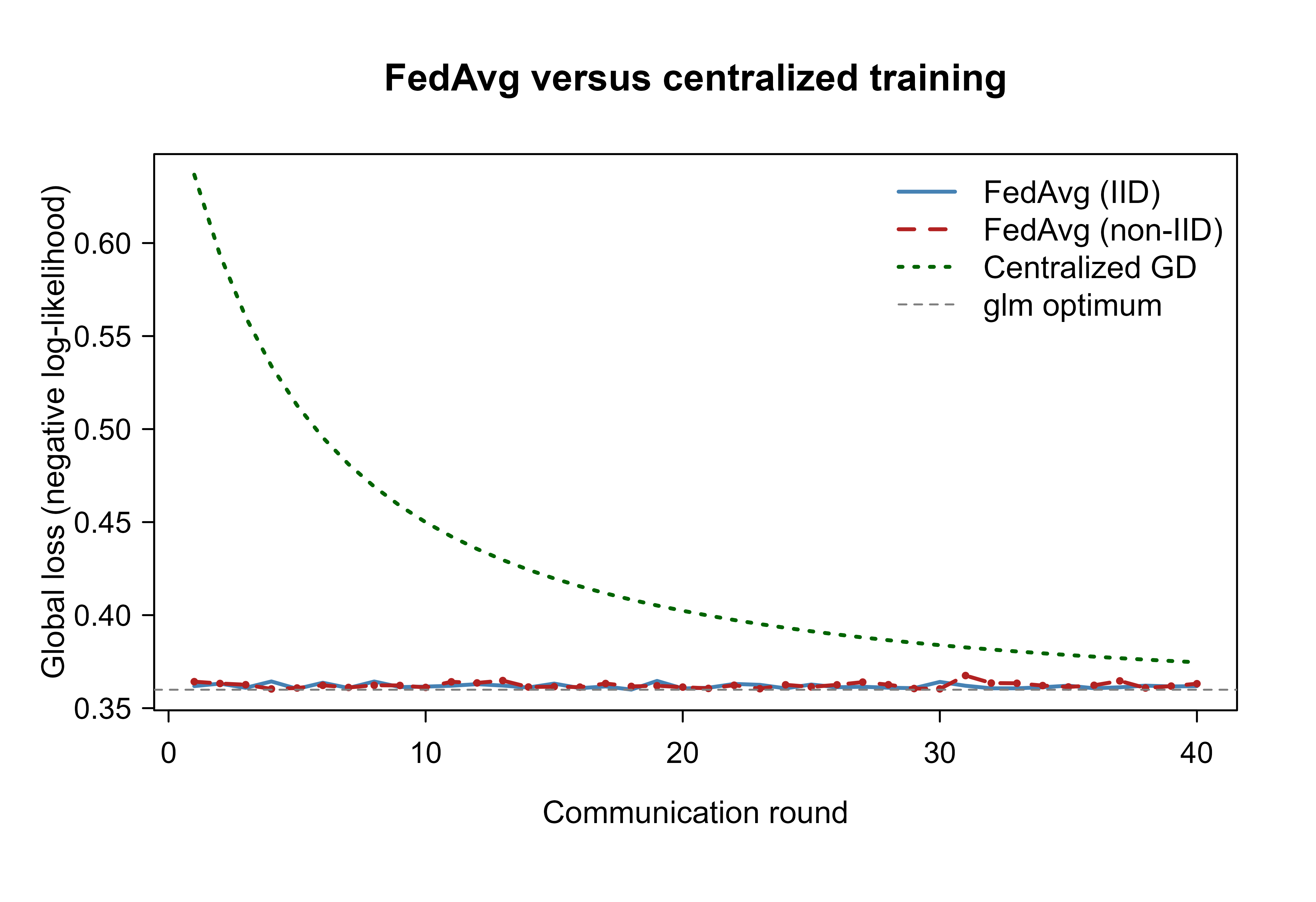
Figure 56.1 plots the global loss against the communication round for all three runs, with the glm optimum drawn as a dashed floor. The centralized baseline here is full-batch gradient descent, which takes exactly one parameter step per round and so descends gradually toward the optimum. FedAvg reaches near-optimal loss almost immediately, because each of its rounds packs several epochs of mini-batch updates inside every client before a single message is exchanged. That is the FedAvg bargain made visible: a great deal of local computation per expensive communication round. The headline result is that FedAvg on IID data settles at the pooled-data optimum without any record leaving its client.

The instructive contrast is between the two FedAvg curves. The IID run sits right on the optimum, while the non-IID run is noisier and plateaus at a visibly higher loss. The mechanism is the interaction flagged in Section 56.4: because only a couple of label-skewed clients are sampled each round, the average update is a biased estimate of the global gradient (a round that happens to draw two mostly-positive clients pulls the model the wrong way). Under the IID split the sampled clients all look like the population, so sampling adds variance but no bias.

ylim <- range(c(fed_iid$loss, fed_noniid$loss, cen$loss, glm_loss))
plot(seq_len(rounds), fed_iid$loss, type = "l", lwd = 2, col = "steelblue",
     ylim = ylim, xlab = "Communication round",
     ylab = "Global loss (negative log-likelihood)",
     main = "FedAvg versus centralized training")
lines(seq_len(rounds), fed_noniid$loss, lwd = 2, lty = 2, col = "firebrick")
points(seq_len(rounds), fed_noniid$loss, pch = 20, col = "firebrick", cex = 0.6)
lines(seq_len(rounds), cen$loss, lwd = 2, lty = 3, col = "darkgreen")
abline(h = glm_loss, lty = 2, col = "grey50")
legend("topright", bty = "n",
       legend = c("FedAvg (IID)", "FedAvg (non-IID)",
                  "Centralized GD", "glm optimum"),
       col = c("steelblue", "firebrick", "darkgreen", "grey50"),
       lty = c(1, 2, 3, 2), lwd = c(2, 2, 2, 1))

Figure 56.1: Global logistic loss versus communication round under client sampling (two of ten clients per round). FedAvg reaches the pooled-data glm optimum (dashed floor) in very few rounds because each round runs several local epochs per client, far outpacing the per-round full-batch centralized baseline (dotted). FedAvg on non-IID data (dashed line with points) is noisier and plateaus higher than the IID run (solid), because sampling a few label-skewed clients yields biased average updates.

56.6.2 Local epochs and the communication tradeoff

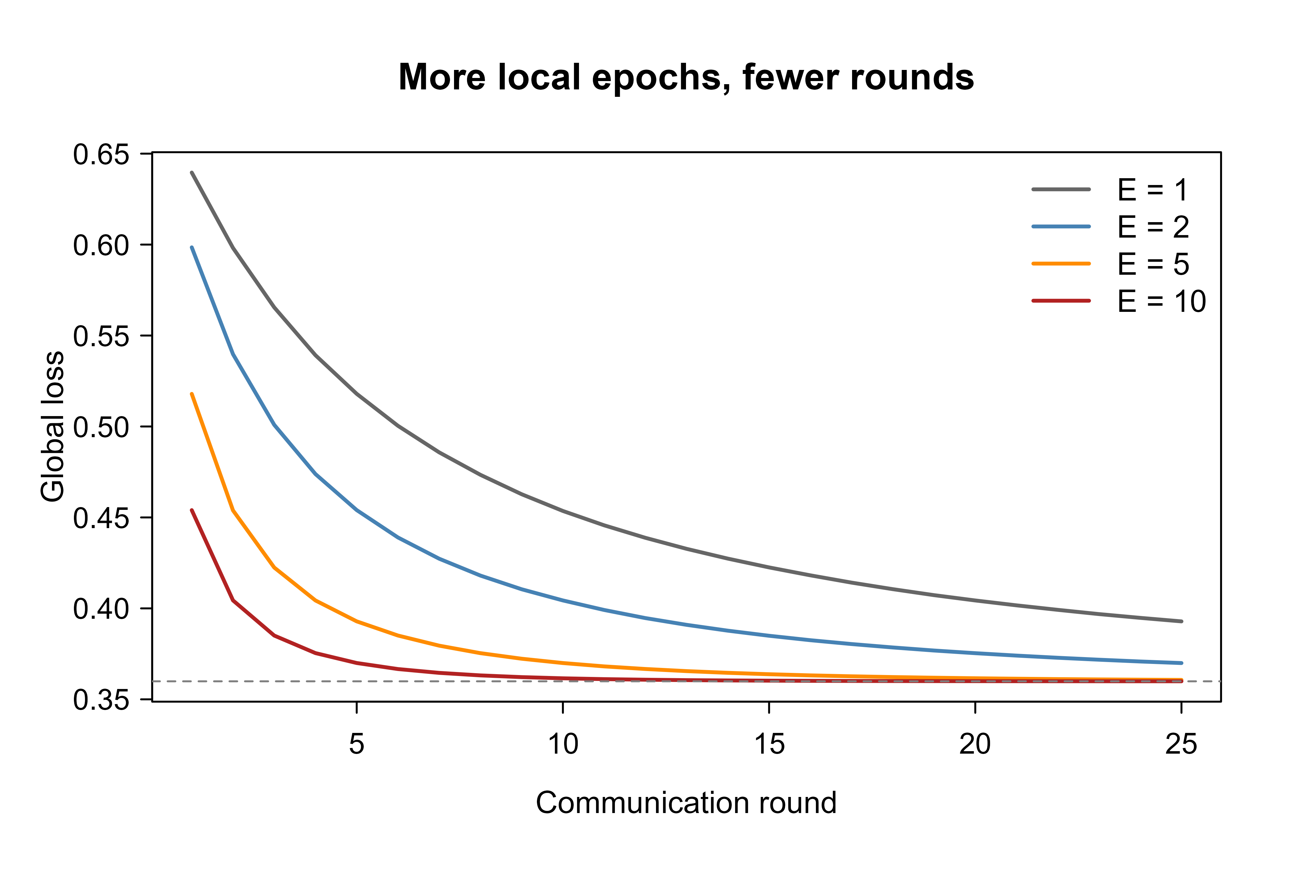
The demo used \(E = 3\) local epochs. To see the communication lever directly, we rerun FedAvg on the IID partition (full participation, so we isolate the effect of local work) for several values of \(E\). More local work per round should reach a given loss in fewer rounds. Figure 56.2 shows the loss curves; larger \(E\) drops the loss faster per round. On this well-behaved convex problem the gains keep accruing with \(E\), but on heterogeneous data the curve for large \(E\) eventually stops improving or oscillates once client drift overtakes the savings, which is the turnover discussed next.

# Use a smaller learning rate and larger batches here so that a single local
# epoch is not already enough to converge; this lets the value of E show.
E_grid <- c(1, 2, 5, 10)
cols   <- c("grey40", "steelblue", "darkorange", "firebrick")
runs_E <- lapply(E_grid, function(e)
  fedavg(iid_clients, X, y, rounds = 25, E = e, eta = 0.05, batch_size = 64))

ylim2 <- range(c(sapply(runs_E, function(r) r$loss), glm_loss))
plot(seq_len(25), runs_E[[1]]$loss, type = "l", lwd = 2, col = cols[1],
     ylim = ylim2, xlab = "Communication round",
     ylab = "Global loss", main = "More local epochs, fewer rounds")
for (j in 2:length(E_grid))
  lines(seq_len(25), runs_E[[j]]$loss, lwd = 2, col = cols[j])
abline(h = glm_loss, lty = 2, col = "grey50")
legend("topright", bty = "n", legend = paste0("E = ", E_grid),
       col = cols, lwd = 2)

Figure 56.2: Effect of local epochs E on FedAvg convergence (IID data). Each curve is the global loss per communication round for a different amount of local work. More local epochs reduce the loss faster per round, which is how FedAvg trades cheap on-client computation for expensive communication.

56.6.3 A differentially private variant

Finally we add central differential privacy to the aggregation: clip each client’s update direction (how far it moved from the global model) to a fixed norm, then add Gaussian noise before averaging. This is the clip-and-noise recipe from Section 56.5, and it lets us measure the accuracy cost of privacy on this problem.

fedavg_dp <- function(clients, X, y, rounds, E, eta, batch_size,
                      clip = 1.0, noise_sd = 0.0) {
  w_global <- rep(0, ncol(X))
  n_k <- sapply(clients, length)
  loss_hist <- numeric(rounds)
  for (t in seq_len(rounds)) {
    deltas <- lapply(clients, function(idx) {
      w_k <- local_update(w_global, X[idx, , drop = FALSE], y[idx],
                          E, eta, batch_size)
      delta <- w_k - w_global                       # update direction
      norm  <- sqrt(sum(delta^2))
      delta * min(1, clip / norm)                   # clip to norm <= clip
    })
    D <- do.call(cbind, deltas)
    avg_delta <- as.vector(D %*% (n_k / sum(n_k)))
    avg_delta <- avg_delta + rnorm(length(avg_delta), sd = noise_sd)  # DP noise
    w_global  <- w_global + avg_delta
    loss_hist[t] <- logistic_loss(w_global, X, y)
  }
  list(w = w_global, loss = loss_hist)
}

dp_none <- fedavg_dp(iid_clients, X, y, rounds, E, eta, batch_size,
                     clip = 1.0, noise_sd = 0.00)
dp_lo   <- fedavg_dp(iid_clients, X, y, rounds, E, eta, batch_size,
                     clip = 1.0, noise_sd = 0.02)
dp_hi   <- fedavg_dp(iid_clients, X, y, rounds, E, eta, batch_size,
                     clip = 1.0, noise_sd = 0.08)

round(c(no_noise = tail(dp_none$loss, 1),
        low_noise = tail(dp_lo$loss, 1),
        high_noise = tail(dp_hi$loss, 1)), 4)
#>   no_noise  low_noise high_noise 
#>     0.3602     0.3601     0.3614

56.6.4 Comparing the variants

Table 56.1 collects the final global loss and a simple classification accuracy for every method we ran. It quantifies the three lessons of the chapter: IID FedAvg reaches the pooled-data optimum, sampling label-skewed clients (non-IID) costs both loss and accuracy, and differential privacy trades accuracy for protection in proportion to the noise added. The differential-privacy rows use full client participation to isolate the noise effect, so they should be read against the IID run rather than the sampled non-IID run.

accuracy <- function(w) mean((sigmoid(as.vector(X %*% w)) > 0.5) == y)

comp <- data.frame(
  Method = c("Centralized GD", "glm (pooled optimum)",
             "FedAvg (IID)", "FedAvg (non-IID)",
             "FedAvg + DP (low noise)", "FedAvg + DP (high noise)"),
  `Final loss` = round(c(tail(cen$loss, 1), glm_loss,
                         tail(fed_iid$loss, 1), tail(fed_noniid$loss, 1),
                         tail(dp_lo$loss, 1), tail(dp_hi$loss, 1)), 4),
  Accuracy = round(c(accuracy(cen$w), accuracy(coef(glm_fit)),
                     accuracy(fed_iid$w), accuracy(fed_noniid$w),
                     accuracy(dp_lo$w), accuracy(dp_hi$w)), 4),
  check.names = FALSE
)

knitr::kable(
  comp,
  caption = "Final global loss and accuracy across training schemes on the same synthetic logistic problem. FedAvg on IID data reaches the pooled glm optimum; under client sampling, non-IID partitioning costs both loss and accuracy because the sampled clients give a biased average update; and adding differential-privacy noise to the aggregation (with full participation, to isolate the noise) trades accuracy for protection as the noise grows.",
  booktabs = TRUE
)

Table 56.1: Final global loss and accuracy across training schemes on the same synthetic logistic problem. FedAvg on IID data reaches the pooled glm optimum; under client sampling, non-IID partitioning costs both loss and accuracy because the sampled clients give a biased average update; and adding differential-privacy noise to the aggregation (with full participation, to isolate the noise) trades accuracy for protection as the noise grows.

Method	Final loss	Accuracy
Centralized GD	0.3747	0.8360
glm (pooled optimum)	0.3599	0.8362
FedAvg (IID)	0.3618	0.8355
FedAvg (non-IID)	0.3631	0.8330
FedAvg + DP (low noise)	0.3601	0.8362
FedAvg + DP (high noise)	0.3614	0.8365

56.7 Practical guidance and pitfalls

The simulation is small, but every choice it exposed scales up to real deployments. A handful of points are worth carrying forward.

Tune local epochs and heterogeneity together. The single most important hyperparameter is the amount of local work \(E\). Raise it to cut communication rounds, but watch the non-IID loss curve: when added local epochs stop lowering the loss or start making it bounce, drift has overtaken the savings and you should back off or switch to a drift-correcting method like FedProx or SCAFFOLD. There is no universal best \(E\); it depends on how heterogeneous your clients are.

When to use this

Reach for federated learning when data genuinely cannot be centralized (regulation, privacy, ownership, or bandwidth) and the value lies in combining it. If you are allowed to pool the data, pool it. Centralized training is simpler, faster, and strictly easier to debug, and the demo shows the best federated outcome merely matches it.

Do not equate “data stayed put” with “privacy achieved.” Model updates leak information, and a determined adversary can exploit them. If privacy is a real requirement and not a slogan, budget for differential privacy from the start, expect to pay accuracy for it, and add secure aggregation so the server never inspects an individual client’s update. Decide explicitly whether you trust the server (central DP, better accuracy) or not (local DP, stronger guarantee).

Warning

Because clients train on data the server never sees, a malicious or malfunctioning client can poison the global model with crafted updates, and plain averaging gives every client equal sway. In any open or low-trust federation, replace the mean with a robust aggregation rule (coordinate-wise median, trimmed mean, or Krum) and clip update norms so no single client can dominate a round.

Mind the systems realities the demo glossed over. Real clients are intermittently available, run at wildly different speeds, and number in the thousands or millions, so you will sample a small fraction each round and set deadlines that drop stragglers. Model size \(d\) drives every uplink message, so for large models, compression (quantization, sparsification) is not optional. And monitoring is genuinely hard: you cannot inspect the data that produced a bad update, so build evaluation on a held-out, server-side proxy set and track per-round global metrics, exactly the global-loss curve the demo plotted, as your primary health signal.

56.8 Further reading

The founding paper is McMahan, Moore, Ramage, Hampson, and Aguera y Arcas, “Communication-Efficient Learning of Deep Networks from Decentralized Data” (2017), which introduced FedAvg and the IID-versus-non-IID experiments this chapter mirrors. For the non-IID problem and its remedies, see Li, Sahu, Zaheer, Sanjabi, Talwalkar, and Smith on FedProx (2020) and Karimireddy, Kale, Mohri, Reddi, Stich, and Suresh on SCAFFOLD (2020). The broad survey by Kairouz, McMahan, and many coauthors, “Advances and Open Problems in Federated Learning” (2021), is the standard reference map of the whole field. For privacy, the foundational text is Dwork and Roth, The Algorithmic Foundations of Differential Privacy (2014), with the deep-learning connection in Abadi and colleagues, “Deep Learning with Differential Privacy” (2016); secure aggregation is due to Bonawitz and colleagues (2017). A readable book-length treatment of systems and applications is Yang, Liu, Chen, and Tong, Federated Learning (2019).