Advanced Data Analysis

Nguyen, Mike

27 Dimension Reduction

Modern data sets often arrive with far more measured features than we can comfortably reason about: gene expression panels with thousands of probes, images with one variable per pixel, surveys with hundreds of questions. Working directly in such a high-dimensional space is awkward. Plots become impossible, models overfit, distances between points lose meaning, and storage and computation costs grow quickly. Dimension reduction is the family of techniques that responds to this problem by replacing the original features with a much smaller set of new ones that still capture most of what matters in the data.

The guiding intuition is that high-dimensional data usually live, at least approximately, on a much lower-dimensional shape. The pixels of a face photograph are not independent: lighting, pose, and identity vary in a handful of coordinated ways, even though there are tens of thousands of pixels. If we can find those few underlying coordinates, we can describe each observation compactly, visualize the data, remove noise, and feed cleaner inputs to downstream models. The art is in deciding what “most of what matters” should mean, and the methods in this chapter differ mainly in how they answer that question.

We begin with principal components analysis (PCA), the workhorse of linear dimension reduction. PCA looks for a small number of directions along which the data vary the most, and it turns out to be the right starting point because so many other methods are either special cases of it, extensions of it, or reactions against its limitations. From there we build outward: aligning two point clouds (Procrustes transformations), bending PCA into curved feature spaces (kernel PCA), making the result interpretable (sparse PCA), respecting non-negativity (non-negative matrix factorization), and finally relaxing the linearity assumption altogether (nonlinear dimension reduction).

Key idea

Almost everything in this chapter reduces to one linear-algebra tool, the singular value decomposition (SVD). If you understand how the SVD gives you PCA, the rest of the chapter is a set of variations on that theme.

27.1 Principal Components

Principal components analysis is worth studying carefully because of its relationship to so many other dimension reduction approaches: understand it well, and you have a lens for understanding the rest.

The core idea is to build a new set of variables, each a linear combination of the original features, that collectively account for the largest possible amount of variation in those features. “A linear combination” simply means a weighted sum, and the weights are what we are solving for. Concretely, we seek the coefficients, called loadings, of the linear combination of our features that maximizes the variance of the resulting new variable.

The first principal component of a set of $p$ features is given by

\[ Z_1 = \phi_{11} X_1 + \phi_{21} X_2 + \dots + \phi_{p1}X_p \]

where the coefficients (loadings) are normalized such that $\sum_{j=1}^p \phi^2_{j1} = 1$. The normalization matters: without it we could inflate the variance arbitrarily just by scaling the weights up, so we constrain the loading vector to have unit length and let only its direction do the work.¹

The next principal component is again a linear combination of the same features, chosen to account for the next largest amount of variation, subject to being orthogonal to the first. We continue in this way, each new component capturing as much of the remaining variation as possible while staying perpendicular to all the ones before it. Orthogonality is what keeps the components from redundantly re-describing the same variation.

Intuition

Picture the data as an elongated cloud of points. The first principal component is the long axis of the cloud, the direction in which the points are most spread out. The second is the longest direction perpendicular to the first, and so on. Keeping only the first few axes is like photographing the cloud from its most informative angle.

27.1.1 The variance-maximization problem and its solution

Before turning to the reconstruction view, it is worth deriving the loadings directly from the variance-maximization statement, because that derivation makes precise what “the direction of greatest spread” means and shows where the eigenvectors come from.

Collect the centered observations as the rows of $\mathbf{X}$ ($n \times p$, columns having sample mean zero) and write the sample covariance matrix as $\mathbf{S} = \tfrac{1}{n}\mathbf{X}^T\mathbf{X}$, a $p \times p$ symmetric positive semidefinite matrix. A candidate component is $\mathbf{X}\phi$ for a unit loading vector $\phi \in \mathbb{R}^p$, and its sample variance is

\[ \operatorname{Var}(\mathbf{X}\phi) = \frac{1}{n}\phi^T \mathbf{X}^T \mathbf{X}\,\phi = \phi^T \mathbf{S}\,\phi . \]

The first principal direction solves

\[ \max_{\phi}\ \phi^T \mathbf{S}\,\phi \quad \text{subject to}\quad \phi^T\phi = 1 . \tag{27.1}\]

Introduce a Lagrange multiplier $\lambda$ for the unit-norm constraint and form $\mathcal{L}(\phi,\lambda) = \phi^T\mathbf{S}\phi - \lambda(\phi^T\phi - 1)$. Setting the gradient to zero,

\[ \frac{\partial \mathcal{L}}{\partial \phi} = 2\mathbf{S}\phi - 2\lambda\phi = 0 \;\Longrightarrow\; \mathbf{S}\phi = \lambda\phi . \tag{27.2}\]

So any stationary point of Equation 27.1 is an eigenvector of $\mathbf{S}$, and at such a point the objective equals $\phi^T\mathbf{S}\phi = \lambda\,\phi^T\phi = \lambda$. The maximum variance is therefore the largest eigenvalue $\lambda_1$, attained by its eigenvector $\phi_1 = \mathbf{v}_1$. The second component maximizes $\phi^T\mathbf{S}\phi$ subject to $\phi^T\phi = 1$ and $\phi^T\mathbf{v}_1 = 0$; the same Lagrangian argument, now with two multipliers, forces $\phi$ to be an eigenvector orthogonal to $\mathbf{v}_1$, and the best choice is $\mathbf{v}_2$ with variance $\lambda_2$. Inductively, the $k$-th loading vector is the $k$-th eigenvector of $\mathbf{S}$, and the $k$-th component has variance $\lambda_k$. This is the Courant-Fischer (Rayleigh quotient) characterization of eigenvalues, and it explains why the singular values, which satisfy $d_k^2 = n\lambda_k$ for the centered $\mathbf{X} = \mathbf{UDV}^T$, rank the directions exactly by variance.

Two views, one answer

The reconstruction problem in Equation 27.3 (minimize squared error of a rank-$q$ fit) and the variance-maximization problem in Equation 27.1 (find directions of greatest spread) have the same solution, the leading eigenvectors of $\mathbf{S}$. The reason is the identity, for a unit direction $\phi$, that the total scatter splits as projected variance plus residual variance, $\tfrac1n\sum_i\|x_i-\bar x\|^2 = \phi^T\mathbf{S}\phi + \tfrac1n\sum_i\|(x_i-\bar x) - \phi\phi^T(x_i-\bar x)\|^2$. Maximizing the first term is the same as minimizing the second.

27.1.2 A more formal view

Having built intuition, we can state the problem precisely. The principal components of a set of features in $R^p$ give a sequence of linear approximations of rank $q \le p$. The number $q$ is the dimension we are reducing to, and the whole point is that a small $q$ can describe the data well.

Recall that we have observations $x_i, i = 1, \dots, n$, where each $x_i$ is $p$-dimensional. We seek the rank-$q$ linear model that represents these vectors, \[x_i \approx f(z_i) = \mu + \mathbf{V}_q z_i,\] where $\mu$ is a $p$-dimensional mean, $\mathbf{V}_q$ is a $p \times q$ matrix with $q$ orthogonal unit vectors as columns, and $z_i$ is a $q$-vector of parameters. Read this equation as: every observation is approximated by a common center $\mu$ plus a combination of $q$ shared directions (the columns of $\mathbf{V}_q$), with the per-observation weights collected in $z_i$.

We choose these pieces to minimize the reconstruction error, the total squared distance between each observation and its approximation:

\[ \underset{\mu, \{z_i \}, \mathbf{V}_q}{\operatorname{min}} \sum_{i = 1}^n ||x_i - \mu - \mathbf{V}_qz_i ||^2 \tag{27.3}\]

This optimization looks intimidating because three things are unknown at once, but two of them have closed-form answers once the third is fixed. It can be shown that, given $\mathbf{V}_q$, we get

\[ \hat{\mu} = \bar{x} \\ \hat{z}_i = \mathbf{V}_q^T (x_i - \bar{x}) \]

In words: the best center is just the sample mean, and the best low-dimensional coordinates for an observation are obtained by centering it and then projecting it onto the chosen directions. The real work, then, is finding $\mathbf{V}_q$; once we have it, everything else follows immediately.

To see why those two pieces take that form, differentiate the objective in Equation 27.3. Holding $\mathbf{V}_q$ and the $z_i$ fixed, the gradient with respect to $\mu$ is $-2\sum_i (x_i - \mu - \mathbf{V}_q z_i)$; setting it to zero gives $\hat\mu = \bar x - \mathbf{V}_q \bar z$, and because the objective is invariant to shifting all $z_i$ by a constant, we may impose $\bar z = 0$, leaving $\hat\mu = \bar x$. Substituting this and writing $\tilde x_i = x_i - \bar x$, each $z_i$ appears in a separate term $\|\tilde x_i - \mathbf{V}_q z_i\|^2$. Its gradient is $-2\mathbf{V}_q^T(\tilde x_i - \mathbf{V}_q z_i)$, and since $\mathbf{V}_q^T\mathbf{V}_q = \mathbf{I}_q$ (orthonormal columns), setting it to zero gives $\hat z_i = \mathbf{V}_q^T \tilde x_i$, the orthogonal projection onto the column space of $\mathbf{V}_q$.

Plugging $\hat\mu$ and $\hat z_i$ back in collapses the objective to a function of $\mathbf{V}_q$ alone,

\[ \sum_{i=1}^n \big\| \tilde x_i - \mathbf{V}_q \mathbf{V}_q^T \tilde x_i \big\|^2 = \operatorname{trace}\!\big[ \tilde{\mathbf{X}}^T \tilde{\mathbf{X}} (\mathbf{I}_p - \mathbf{V}_q\mathbf{V}_q^T) \big], \tag{27.4}\]

where $\mathbf{P} = \mathbf{V}_q\mathbf{V}_q^T$ is the rank-$q$ orthogonal projector onto the chosen subspace. Minimizing Equation 27.4 is the same as maximizing $\operatorname{trace}(\mathbf{V}_q^T\tilde{\mathbf{X}}^T\tilde{\mathbf{X}}\,\mathbf{V}_q)$ over orthonormal $\mathbf{V}_q$, which by the Ky Fan theorem is solved by taking the top $q$ eigenvectors of $\tilde{\mathbf{X}}^T\tilde{\mathbf{X}}$, exactly the leading right singular vectors. This is the precise sense in which the reconstruction and variance views coincide.

27.1.2.1 Finding the directions with the SVD

We can find $\mathbf{V}_q$ as follows. First, we stack the centered observations into the rows of an $n \times p$ matrix, $\mathbf{X}$, then compute its singular value decomposition,

\[ \mathbf{X} = \mathbf{UDV}^T \]

The SVD factors any matrix into three interpretable pieces:

$\mathbf{U}$ is an $n \times p$ orthogonal matrix ($\mathbf{U^TU} = I_p$), whose columns $\mathbf{u}_j$ are the left singular vectors,
$\mathbf{V}$ is a $p \times p$ orthogonal matrix ($\mathbf{V^T V} = \mathbf{I}_p$) with columns $\mathbf{v}_j$ called the right singular vectors,
$\mathbf{D}$ is a $p \times p$ diagonal matrix, with diagonal elements $d_1 \ge d_2 \ge \dots d_p \ge 0$, known as the singular values.

The singular values are ordered from largest to smallest, and that ordering is exactly what we need: it ranks the directions by how much variation they carry. The directions we want are therefore the leading columns of $\mathbf{V}$. Concretely, $\mathbf{V}_q$ consists of the first $q$ columns of $\mathbf{V}$, and in this case the columns of $\mathbf{UD}$ are called the principal components of $\mathbf{X}$.

Putting it together, the $n$ optimal $\hat{z}_i$ are given by the first $q$ principal components: the $n$ rows of the $n \times q$ matrix $\mathbf{U}_q \mathbf{D}_q = \mathbf{XV}_q = \mathbf{Z}$, where $\mathbf{Z}$ is the $n \times q$ matrix of principal component scores. The scores are the new low-dimensional coordinates of each observation, the compact description we set out to find.

Two facts are worth keeping in mind as you connect PCA to other material. First, the columns of $\mathbf{V}$ are equivalent to the eigenvectors of the sample covariance matrix, so PCA can be described either through the SVD of the data or through the eigendecomposition of its covariance, and you will see both in the literature.

Second, a practical question: how many components should we keep? A useful diagnostic is to compare the variation captured by the real data against the variation captured when the data are deliberately scrambled. You randomize the pixels (or feature values) across samples to destroy any real structure, run the same decomposition, and compare. The number of components whose singular values rise meaningfully above the randomized baseline is roughly the number worth keeping; at the point where the real and randomized curves meet, the extra components are capturing noise rather than signal. Hastie, Friedman, and Tibshirani (2001) (14.24) illustrate exactly this comparison, showing the singular values for randomized data alongside those for the actual images.

Tip

The scrambling comparison is more honest than the familiar “look for an elbow in the scree plot” rule, because it gives you a concrete null expectation for how much variance a meaningless direction should explain.

27.1.2.2 Optimality, variance accounted for, and complexity

The Eckart-Young-Mirsky theorem makes the optimality of PCA exact: among all rank-$q$ matrices $\mathbf{B}$, the truncated SVD $\mathbf{X}_q = \mathbf{U}_q\mathbf{D}_q\mathbf{V}_q^T$ minimizes both the Frobenius error $\|\mathbf{X} - \mathbf{B}\|_F$ and the spectral-norm error $\|\mathbf{X}-\mathbf{B}\|_2$, with optimal values

\[ \|\mathbf{X} - \mathbf{X}_q\|_F^2 = \sum_{k=q+1}^{p} d_k^2, \qquad \|\mathbf{X}-\mathbf{X}_q\|_2 = d_{q+1}. \]

Dividing the leading sum by the total, the fraction of variance explained by the first $q$ components is $\sum_{k=1}^q d_k^2 \big/ \sum_{k=1}^p d_k^2 = \sum_{k=1}^q \lambda_k \big/ \sum_{k=1}^p \lambda_k$, which is the quantity a cumulative scree plot reports. Choosing $q$ to reach a target such as 90 percent is the most common rule of thumb; the scrambling baseline above and cross-validated reconstruction error (hold out entries of $\mathbf{X}$, reconstruct, measure error) are more principled alternatives.

Computationally, forming $\mathbf{S}$ and taking its eigendecomposition costs $O(np^2 + p^3)$, while a thin SVD of $\mathbf{X}$ costs $O(np\min(n,p))$; when only $q \ll p$ components are needed, randomized or Lanczos/truncated SVD reduces this to roughly $O(npq)$. Forming $\mathbf{S}$ explicitly squares the condition number, so for accuracy prefer the SVD of $\mathbf{X}$ directly over the eigendecomposition of $\mathbf{X}^T\mathbf{X}$.

Failure modes

PCA is a second-moment method, so it can mislead when the interesting structure is not captured by variance. It is not scale invariant (recall the standardization footnote); a single high-variance feature or a few gross outliers can hijack the leading components, since squared error rewards fitting large deviations. Variance is also not the same as class separation, so the top components need not be the best features for a downstream classifier (that is the job of methods like LDA). And when $p \gg n$ the leading sample eigenvectors are inconsistent estimates of the population directions unless the signal eigenvalues are large enough, a phenomenon made precise by random-matrix theory (the Baik-Ben Arous-Peche phase transition).

We can confirm the central claim, that the leading right singular vector both maximizes variance and minimizes reconstruction error, with a tiny simulation.

Show code

set.seed(1)
n <- 200; p <- 5
X <- scale(matrix(rnorm(n * p), n, p) %*% matrix(rnorm(p * p), p, p),
           center = TRUE, scale = FALSE)
sv <- svd(X)
v1 <- sv$v[, 1]                       # leading right singular vector

# variance along v1 vs. many random unit directions
var_v1 <- var(X %*% v1)
rand_dir <- function() { u <- rnorm(p); u <- u / sqrt(sum(u^2)); var(X %*% u) }
max_random <- max(replicate(2000, rand_dir()))
c(variance_along_v1 = var_v1, best_of_random = max_random)
#> variance_along_v1    best_of_random 
#>          21.35613          20.52290

# rank-1 reconstruction error equals sum of squared trailing singular values
Xq <- sv$u[, 1] %*% t(sv$v[, 1]) * sv$d[1]
c(reconstruction = sum((X - Xq)^2), trailing_sv2 = sum(sv$d[-1]^2))
#> reconstruction   trailing_sv2 
#>       1711.475       1711.475

The variance along $\mathbf{v}_1$ exceeds that of every random direction, and the rank-1 reconstruction error matches $\sum_{k\ge 2} d_k^2$, as Equation 27.4 and the Eckart-Young theorem predict.

The remaining sections all start from this PCA machinery and modify one ingredient at a time.

27.1.3 Procrustes Transformations

A notion closely related to PCA arises when, instead of compressing one data set, we want to overlay two of them: given one set of points, find the translation and rotation that best lines it up with another. This is a Procrustes transformation, named after the mythological figure who stretched or trimmed travelers to fit his bed. Here we are gently rotating and shifting one cloud of points to match another, not deforming it.

Say we have two matrices, $\mathbf{X}_1$ and $\mathbf{X}_2$, and we want to transform $\mathbf{X}_1$ to match $\mathbf{X}_2$ as closely as possible. We pose this as

\[ \underset{\mu, \mathbf{R}}{\operatorname{min}} ||\mathbf{X}_2 - (\mathbf{X}_1 \mathbf{R} + \mathbf{1} \mu^T) ||_F \]

where the ingredients are

$\mathbf{X}_1, \mathbf{X}_2$, which are $n \times p$ matrices,
$\mathbf{R}$, an orthonormal $p \times p$ rotation matrix, and
$\mu$, a $p$-vector that supplies the shift (translation).

The notation $||\mathbf{A}||_F$ is the Frobenius matrix norm, defined through $||\mathbf{A}||_F^2 \equiv trace(\mathbf{A^T A})$ for a matrix $\mathbf{A}$. It is just the matrix version of ordinary Euclidean length: the square root of the sum of all squared entries.²

This problem has an elegant closed-form solution, and (no surprise given the theme of this chapter) it runs through the SVD. Let $\bar{x}_1$ and $\bar{x}_2$ be the column mean vectors of $\mathbf{X}_1$ and $\mathbf{X}_2$, and let $\tilde{\mathbf{X}}_1$ and $\tilde{\mathbf{X}}_2$ be the corresponding data matrices with those means removed. We then take the SVD of $\tilde{\mathbf{X}}_1^T\tilde{\mathbf{X}}_2 = \mathbf{UDV}^T$. The optimal rotation and shift are

\[ \hat{\mathbf{R}} = \mathbf{UV}^T \\ \hat{\mu} = \bar{x}_2 - \hat{\mathbf{R}}^T \bar{x}_1 \]

The first line says the best rotation comes straight from the singular vectors; the second says that once you know how to rotate, the right shift is simply whatever lines the two centers up. We will see this solution reappear inside sparse PCA below.

To derive this, note first that for any fixed $\mathbf{R}$ the optimal $\mu$ centers the residual, $\hat\mu = \bar x_2 - \mathbf{R}^T \bar x_1$ (differentiate the objective in $\mu$ and set to zero, exactly as for PCA’s mean), so we may work with the centered matrices $\tilde{\mathbf{X}}_1, \tilde{\mathbf{X}}_2$ and drop the translation. Expanding the squared Frobenius norm and using $\mathbf{R}^T\mathbf{R} = \mathbf{I}$,

\[ \|\tilde{\mathbf{X}}_2 - \tilde{\mathbf{X}}_1\mathbf{R}\|_F^2 = \|\tilde{\mathbf{X}}_2\|_F^2 + \|\tilde{\mathbf{X}}_1\|_F^2 - 2\operatorname{trace}\!\big(\mathbf{R}^T \tilde{\mathbf{X}}_1^T \tilde{\mathbf{X}}_2\big), \]

so minimizing over orthonormal $\mathbf{R}$ is equivalent to maximizing $\operatorname{trace}(\mathbf{R}^T \mathbf{C})$ with $\mathbf{C} = \tilde{\mathbf{X}}_1^T \tilde{\mathbf{X}}_2$. Take the SVD $\mathbf{C} = \mathbf{U}\mathbf{D}\mathbf{V}^T$. Then

\[ \operatorname{trace}(\mathbf{R}^T\mathbf{U}\mathbf{D}\mathbf{V}^T) = \operatorname{trace}(\mathbf{D}\,\mathbf{V}^T\mathbf{R}^T\mathbf{U}) = \sum_k d_k\, m_{kk}, \quad \mathbf{M} = \mathbf{V}^T\mathbf{R}^T\mathbf{U}, \]

where $\mathbf{M}$ is orthonormal, so $|m_{kk}| \le 1$. Since every $d_k \ge 0$, the sum is maximized by $m_{kk} = 1$ for all $k$, i.e. $\mathbf{M} = \mathbf{I}$, which gives $\hat{\mathbf{R}} = \mathbf{U}\mathbf{V}^T$. (If a proper rotation, $\det \hat{\mathbf{R}} = +1$, is required so reflections are excluded, the Kabsch correction replaces the last column relation by $\hat{\mathbf{R}} = \mathbf{U}\,\mathrm{diag}(1,\dots,1,\det(\mathbf{U}\mathbf{V}^T))\,\mathbf{V}^T$.) This is the orthogonal Procrustes solution, and the trace-maximization step is the same device that solved PCA above.

27.1.4 Kernel Principal Components

PCA finds the best flat (linear) low-dimensional approximation. But data often bend: points may lie on a curved surface that no straight axis can follow. We can extend principal components to capture such curvature, leading to principal curves and surfaces (for example Hastie, Friedman, and Tibshirani (2001) 14.5.2) and, more generally, to kernel principal components (KPCA).

The idea behind KPCA is to nonlinearly transform the features and then perform the SVD in that transformed feature space. By bending the space first, a curved structure in the original coordinates can become flat in the new ones, where ordinary PCA works again.

To see how this is possible without ever writing down the transformation explicitly, start from a reformulation of plain PCA. If $\mathbf{X} = \mathbf{UDV}^T$, then the so-called Gram matrix is $\mathbf{K} \equiv \mathbf{XX}^T$, which collects the inner products between all pairs of observations. If $\mathbf{X}$ is not centered, we can center it using $\tilde{\mathbf{X}} = (\mathbf{I} - \mathbf{M}) \mathbf{X}$, where $\mathbf{M} = (1/n)\mathbf{11}^T$, which yields the double-centered Gram matrix:

\[ \tilde{\mathbf{K}} = (\mathbf{I} - \mathbf{M}) \mathbf{K(I-M)} = \mathbf{UD^2 U^T} \]

Setting $\mathbf{Z = UD}$ then recovers the principal component scores. The key observation is that this is essentially doing PCA through the covariance/Gram structure: we never needed the raw features, only their inner products.

Kernel PCA follows exactly the same procedure but swaps in a different matrix $\mathbf{K}$. Instead of ordinary inner products, we interpret $\mathbf{K} = \{ K(x_i, x_{i'})\}$ as a kernel matrix whose entries are inner products of the transformed features, $K(x_i, x_{i'}) = \langle \phi (x_i), \phi(x_{i'})\rangle$. The function $\phi$ is the nonlinear feature map, but the so-called kernel trick is that we only ever evaluate $K$, never $\phi$ itself.³ We then find the eigenvectors ($\mathbf{U}$) and eigenvalues ($\mathbf{D}$) of this matrix, again form $\mathbf{Z = UD}$, and can show that the $i$-th element of the $m$-th component $\mathbf{z}_m$ (the $m$-th column of $\mathbf{Z}$) is

\[ z_{im} = \sum_{j=1}^N \alpha_{jm} K(x_i, x_j) \]

where the coefficients are $\alpha_{jm} = u_{jm}/d_m$. In other words, each observation’s score is a kernel-weighted combination of its similarities to all the training points.

27.1.4.1 Why the Gram-matrix eigenvectors suffice

The reason KPCA can work entirely with $\mathbf{K}$ is a duality between the covariance and Gram matrices. In feature space, let the (centered) rows be $\phi(x_i)^T$ stacked into $\mathbf{\Phi}$. PCA there would diagonalize the covariance $\mathbf{C} = \tfrac1n \mathbf{\Phi}^T\mathbf{\Phi}$, whose eigenvectors $\mathbf{w}$ satisfy $\mathbf{C}\mathbf{w} = \lambda\mathbf{w}$. Left-multiplying by $\mathbf{\Phi}$ shows that the Gram matrix $\mathbf{K} = \mathbf{\Phi}\mathbf{\Phi}^T$ shares the nonzero spectrum: if $\mathbf{K}\mathbf{u} = n\lambda\,\mathbf{u}$ then $\mathbf{w} = \mathbf{\Phi}^T\mathbf{u}$ is an eigenvector of $n\mathbf{C}$ with the same eigenvalue. Crucially $\mathbf{w}$ lies in the span of the mapped data, $\mathbf{w} = \sum_j u_j \phi(x_j)$, so it never needs to be formed explicitly. The projection (score) of a point onto $\mathbf{w}$ is then

\[ \langle \mathbf{w}, \phi(x_i)\rangle = \sum_{j} u_{j}\,\langle \phi(x_j),\phi(x_i)\rangle = \sum_j u_{j} K(x_j, x_i), \]

which is exactly $z_{im} = \sum_j \alpha_{jm} K(x_i,x_j)$ once we normalize so that $\|\mathbf{w}\|=1$. The eigenvector $\mathbf{w} = \mathbf{\Phi}^T\mathbf{u}$ has squared norm $\mathbf{u}^T\mathbf{K}\mathbf{u} = n\lambda\,\|\mathbf{u}\|^2 = n\lambda$ when $\mathbf{u}$ is unit-norm, so the scaling $\alpha_{jm} = u_{jm}/d_m$ (with $d_m^2$ the $m$-th eigenvalue of $\mathbf{K}$) is precisely what makes the feature-space loading have unit length. This is why KPCA returns $\mathbf{Z} = \mathbf{U}\mathbf{D}$.

One subtlety: centering must be done in feature space, where $\bar\phi = \tfrac1n\sum_j \phi(x_j)$ is unknown. The double-centering $\tilde{\mathbf{K}} = (\mathbf{I}-\mathbf{M})\mathbf{K}(\mathbf{I}-\mathbf{M})$, with $\mathbf{M} = \tfrac1n\mathbf{1}\mathbf{1}^T$, is not an arbitrary normalization: expanding $\langle \phi(x_i)-\bar\phi,\ \phi(x_j)-\bar\phi\rangle$ produces exactly the four terms of $(\mathbf{I}-\mathbf{M})\mathbf{K}(\mathbf{I}-\mathbf{M})$, so it implements mean-subtraction using inner products alone. For a genuinely new test point one must apply the same centering with the training-set means.

Many kernels are available. One of the most common is the radial (Gaussian) kernel,

\[ K(x,x') = \exp(-||x- x'||^2 /c) \]

but polynomial, linear, hyperbolic tangent, Laplacian, and Bessel kernels, among others, are all used in practice.

Warning

Kernel PCA buys flexibility at a price. Because the feature transformation is nonlinear, you generally cannot invert it to recover the original $x$ from a kernel principal component (the so-called pre-image problem). And there is no way to know in advance which kernel will work best for a given data set, so the choice of kernel and its tuning parameters becomes an empirical question.

27.1.5 Sparse PCA

Ordinary principal components are linear combinations of all $p$ features, which makes them hard to interpret in high-dimensional settings: a component that loads a little on every one of a thousand genes tells you very little. Interpretation becomes much easier if the loading vectors are sparse, meaning most loadings are exactly zero so that each component depends on only a handful of features.

There are several ways to achieve this, but one approach that fits naturally with the rest of statistical learning is to frame it as a penalized regression problem. We treat the components as approximating (fitting) the features, and we add a penalty that pushes loadings toward zero. The sparse principal component loadings are the matrices $\mathbf{\Theta}$ and $\mathbf{V}$ that minimize

\[ \sum_{i= 1}^n ||x_i -\mathbf{\theta V}^T x_i||^2 + \lambda \sum_{k=1}^K ||v_k||^2_2 + \sum_{k=1}^K \lambda_{1k}||v_k||_1 \]

subject to $\mathbf{\Theta}^T\mathbf{\Theta} = \mathbf{I}_K$, where $\mathbf{V}$ and $\mathbf{\Theta}$ are both $p \times K$ matrices. The three terms have clear jobs: the first measures how well the components reconstruct the features, the second is a ridge ($\ell_2$) penalty that stabilizes the solution, and the third is a lasso ($\ell_1$) penalty that drives loadings to exactly zero. Together the last two terms are exactly an elastic net penalty, with the $\ell_1$ part doing the work of encouraging sparseness.

What makes this tractable is that the problem decouples nicely. The pair $\mathbf{\Theta}$ and $\mathbf{V}$ can be estimated by alternating between two familiar subproblems:

When $\mathbf{\Theta}$ is held fixed, solving for $\mathbf{V}$ is just an ordinary elastic net regression.
When $\mathbf{V}$ is held fixed, solving for $\mathbf{\Theta}$ is exactly the Procrustes Transformations problem, which the SVD solves in closed form.

Because each step is something we already know how to do, we can iterate between the two until convergence (Hastie, Friedman, and Tibshirani 2001, 14.5.5). This alternating strategy, fix half the unknowns and solve the other half, recurs throughout the chapter.

When to use this

Reach for sparse PCA when interpretability matters as much as compression, for example when you want to name a component by the few variables that define it, or when $p$ is large and you suspect only a subset of features drives each direction of variation.

27.1.6 Non-negative Matrix Factorization

Sometimes the data are inherently non-negative (pixel intensities, word counts, amounts purchased), and we would like the building blocks of our decomposition to be non-negative too, so that they can be read as parts that add up rather than directions that cancel out. Ordinary PCA loadings can be positive or negative, which often makes them hard to interpret as physical components. Non-negative matrix factorization (NMF) enforces non-negativity throughout. Hastie, Friedman, and Tibshirani (2001, 14.6) describe such a method due to Lee and Seung (1999).

Assume we have an $n \times p$ matrix $\mathbf{X}$ and seek to approximate it by

\[ \mathbf{X} \approx \mathbf{WH} \]

where $\mathbf{W}$ is $n \times r$, $\mathbf{H}$ is $r \times p$, and the inner dimension satisfies $r \le \max(n,p)$. All elements of $\mathbf{X}$, $\mathbf{W}$, and $\mathbf{H}$ are assumed to be non-negative. We then find $\mathbf{W}$ and $\mathbf{H}$ that maximize

\[ \sum_{i=1}^n \sum_{j=1}^p [x_{ij} \log(\mathbf{WH})_{ij} - (\mathbf{WH})_{ij}] \]

This objective is not arbitrary: it is the log-likelihood of a model in which each $x_{ij}$ is a Poisson random variable with mean (intensity) $(\mathbf{WH})_{ij}$, which is a natural choice for count-like, non-negative data. The columns of $\mathbf{W}$ are usually the quantities of primary interest, since they present the primary non-negative components in the data: the recurring parts (a facial feature, a topic, a spectral signature) out of which each observation is additively built.⁴

27.1.6.1 The multiplicative update rules

Maximizing the Poisson log-likelihood is equivalent to minimizing the generalized Kullback-Leibler divergence $D(\mathbf{X}\,\|\,\mathbf{W}\mathbf{H}) = \sum_{ij}\big[x_{ij}\log\frac{x_{ij}}{(\mathbf{WH})_{ij}} - x_{ij} + (\mathbf{WH})_{ij}\big]$, which differs from the objective above only by terms not involving $\mathbf{W}$ or $\mathbf{H}$. Lee and Seung (1999) derive monotone multiplicative updates for it,

\[ w_{ik} \leftarrow w_{ik}\,\frac{\sum_{j} h_{kj}\, x_{ij}/(\mathbf{WH})_{ij}}{\sum_{j} h_{kj}}, \qquad h_{kj} \leftarrow h_{kj}\,\frac{\sum_{i} w_{ik}\, x_{ij}/(\mathbf{WH})_{ij}}{\sum_{i} w_{ik}} . \tag{27.5}\]

These arise from a majorize-minimize (EM-like) argument. Using the concavity of the logarithm with auxiliary weights $\rho_{ikj} = w_{ik}h_{kj}/(\mathbf{WH})_{ij}$ (which sum to one over $k$), Jensen’s inequality gives a lower bound on the log term that is tight at the current iterate; maximizing that surrogate in closed form yields Equation 27.5. Two properties follow. First, the updates are purely multiplicative, so starting from strictly positive $\mathbf{W},\mathbf{H}$ they preserve non-negativity automatically, with no projection step. Second, each update cannot increase the divergence, so the algorithm converges monotonically; it converges to a stationary point, not necessarily the global optimum, which is the algorithmic counterpart of the non-uniqueness warned about below. (For the squared-error objective $\|\mathbf{X}-\mathbf{WH}\|_F^2$ the analogous updates replace the ratio kernels by $\mathbf{X}\mathbf{H}^T \!\big/ \mathbf{W}\mathbf{H}\mathbf{H}^T$ and $\mathbf{W}^T\mathbf{X} \!\big/ \mathbf{W}^T\mathbf{W}\mathbf{H}$, elementwise.) The cost per iteration is $O(npr)$, the same order as one alternating step of PCA-style methods.

Warning

The factorization into $\mathbf{W}$ and $\mathbf{H}$ is generally not unique, so different runs (or different initializations) can give different but equally valid decompositions. The result can still be very useful; just do not over-interpret a single solution as the one true set of parts.

27.1.7 Beyond PCA

PCA also has several relatives that extend or reinterpret the same basic idea, each relaxing or reframing one of its assumptions. We will not develop them here, but it is worth knowing they exist and where to read more:

factor analysis, which models the features as driven by a few latent factors plus feature-specific noise (Hastie, Friedman, and Tibshirani 2001, 14.7.1);
archetypal analysis, which represents observations as mixtures of extreme “archetype” points rather than directions of variance (Hastie, Friedman, and Tibshirani 2001, 14.6.1);
independent component analysis, which seeks components that are statistically independent rather than merely uncorrelated (Hastie, Friedman, and Tibshirani 2001, 14.7.2).

Taken together, the methods in this section share one DNA: find a small number of structured ingredients, recovered through an eigen- or singular-value decomposition, that reconstruct the data well. What changes from method to method is the structure we insist on (orthogonal, sparse, non-negative, independent) and how nonlinear we are willing to be.

27.2 Dimension Reduction in R: A Worked Example

Two claims from the theory deserve a demonstration: that the leading principal components reconstruct the data with controllable error (Section 27.1.1), and that the linearity of ordinary PCA is a real limit that the kernel trick removes. prcomp is base R; kernel PCA lives in kernlab.

27.2.1 PCA: variance and reconstruction

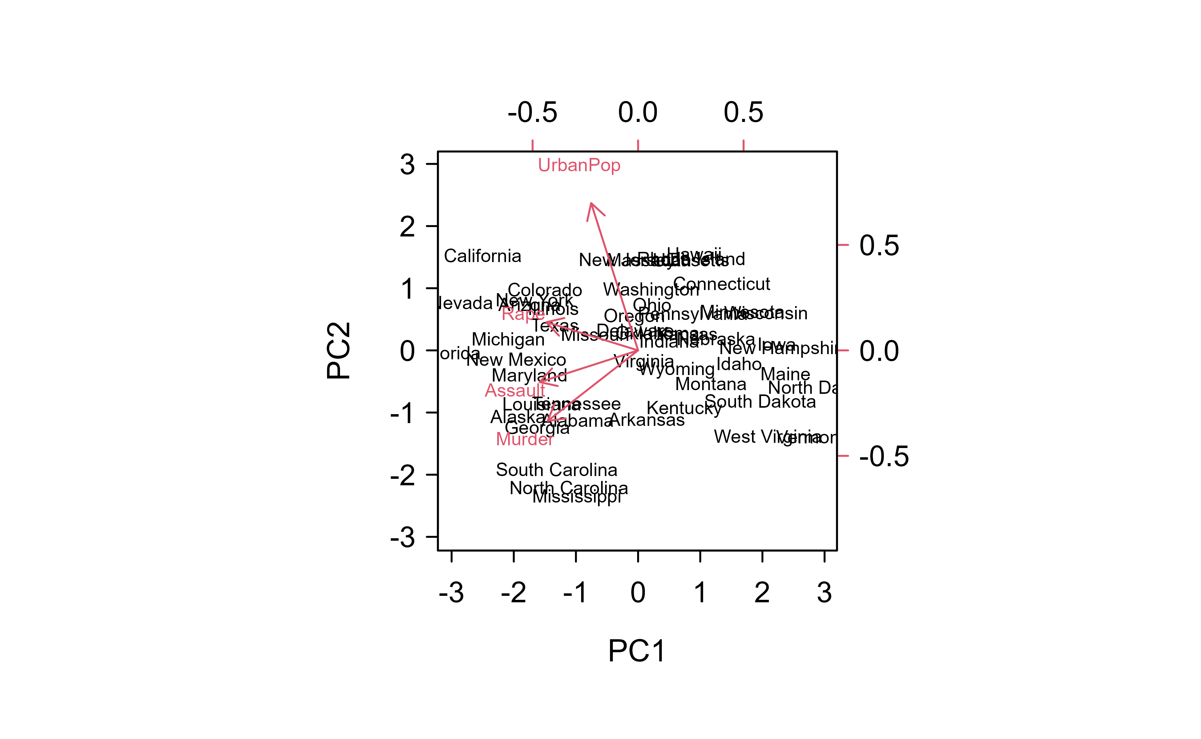
prcomp on standardized data returns components ordered by the variance they capture. The cumulative share tells you how many you can keep:

Show code

X <- scale(USArrests)
pca <- prcomp(X)
round(cumsum(pca$sdev^2) / sum(pca$sdev^2), 3)   # cumulative variance explained
#> [1] 0.620 0.868 0.957 1.000

Two of the four components already carry ~87% of the variance. “Variance explained” is not an abstraction — it is reconstruction accuracy. Project onto the first $k$ components and rotate back, and the mean squared error falls exactly as the discarded variance predicts:

Show code

recon_mse <- sapply(1:4, function(k) {
  Xk <- pca$x[, 1:k, drop = FALSE] %*% t(pca$rotation[, 1:k, drop = FALSE])
  mean((X - Xk)^2)
})
round(recon_mse, 3)                              # MSE using 1..4 components (0 = lossless)
#> [1] 0.372 0.130 0.042 0.000

This is exactly the lever behind PCA-as-compression and PCA-as-denoising: keep the components that hold signal, drop the tail that holds mostly noise.

Show code

biplot(pca, scale = 0, cex = 0.6)

PCA biplot of USArrests: states in the first two principal components, with the original variables as loadings.

27.2.2 When linear PCA is not enough

PCA can only rotate; it cannot bend. Put two classes on concentric rings — separable by radius but by no linear combination of the coordinates — and no principal axis will tell them apart. Kernel PCA maps the data into a feature space first, so a linear axis there corresponds to a curved one here:

Show code

library(kernlab); library(MASS)
set.seed(1)
ring <- function(n, r, s = 0.05) { th <- seq(0, 2*pi, length.out = n); cbind(r*cos(th)+rnorm(n,0,s), r*sin(th)+rnorm(n,0,s)) }
R   <- rbind(ring(150, 1), ring(300, 2.5)); cls <- factor(rep(c("inner", "outer"), c(150, 300)))
lin <- prcomp(R)$x[, 1:2]                                    # ordinary PCA
ker <- rotated(kpca(R, kernel = "rbfdot", kpar = list(sigma = 2), features = 2))  # kernel PCA

sep <- function(z) mean(predict(lda(cls ~ ., data.frame(z, cls)), data.frame(z))$class == cls)
c(linear_PCA = sep(lin), kernel_PCA = sep(ker))             # how separable are the two rings in each space?
#> linear_PCA kernel_PCA 
#>  0.6666667  1.0000000

A classifier built on the two linear principal components is barely above chance, because the rings overlap completely along every straight axis; on the two kernel-PCA components the same classifier is perfect. The kernel “unrolls” the rings into a representation where structure that was hopelessly nonlinear becomes linearly obvious — the same idea that powered the RBF SVM (Chapter 19), now in service of representation rather than classification. When your data plausibly lie on a curved manifold, this is the moment to reach past prcomp toward kernel PCA or the nonlinear methods next.

27.3 Nonlinear Dimension Reduction

Everything so far has been fundamentally linear: even kernel PCA achieves its nonlinearity by mapping into a new space and then doing linear PCA there. Neural-network approaches to the same goal, which learn a nonlinear encoding directly, are taken up in the chapter on autoencoders and representation learning (Chapter 41). The next step is to drop the linearity assumption directly and let the low-dimensional representation follow whatever curved structure (manifold) the data actually lie on. These manifold-learning methods are developed in the chapter on multidimensional scaling and nonlinear dimension reduction (Chapter 31).

Because PCA chases variance, it is sensitive to the scale of the inputs. A feature measured in dollars will dominate one measured in years simply because its numbers are larger. In practice we usually standardize the features (mean zero, unit variance) before running PCA unless the original units are genuinely comparable.↩︎
Restricting $\mathbf{R}$ to be orthonormal is what makes this a rigid alignment. An orthonormal matrix rotates (and possibly reflects) without stretching or shearing, so the shape of the point cloud is preserved and only its orientation and position change.↩︎
This is the same kernel trick that powers support vector machines (Chapter 19): any algorithm written purely in terms of inner products can be made nonlinear by replacing those inner products with a kernel, sidestepping the often impossibly high-dimensional feature map $\phi$.↩︎
The classic illustration is faces: NMF tends to discover localized parts such as eyes, noses, and mouths, whereas PCA produces global “eigenfaces” that look like ghostly whole-face templates. The non-negativity is what forces a parts-based representation.↩︎

# Dimension Reduction {#sec-dimension-reduction} ```{r} #| include: false source("_common.R") ``` Modern data sets often arrive with far more measured features than we can comfortably reason about: gene expression panels with thousands of probes, images with one variable per pixel, surveys with hundreds of questions. Working directly in such a high-dimensional space is awkward. Plots become impossible, models overfit, distances between points lose meaning, and storage and computation costs grow quickly. Dimension reduction is the family of techniques that responds to this problem by replacing the original features with a much smaller set of new ones that still capture most of what matters in the data. The guiding intuition is that high-dimensional data usually live, at least approximately, on a much lower-dimensional shape. The pixels of a face photograph are not independent: lighting, pose, and identity vary in a handful of coordinated ways, even though there are tens of thousands of pixels. If we can find those few underlying coordinates, we can describe each observation compactly, visualize the data, remove noise, and feed cleaner inputs to downstream models. The art is in deciding what "most of what matters" should mean, and the methods in this chapter differ mainly in how they answer that question. We begin with principal components analysis (PCA), the workhorse of linear dimension reduction. PCA looks for a small number of directions along which the data vary the most, and it turns out to be the right starting point because so many other methods are either special cases of it, extensions of it, or reactions against its limitations. From there we build outward: aligning two point clouds (Procrustes transformations), bending PCA into curved feature spaces (kernel PCA), making the result interpretable (sparse PCA), respecting non-negativity (non-negative matrix factorization), and finally relaxing the linearity assumption altogether (nonlinear dimension reduction). ::: {.callout-important title="Key idea"} Almost everything in this chapter reduces to one linear-algebra tool, the singular value decomposition (SVD). If you understand how the SVD gives you PCA, the rest of the chapter is a set of variations on that theme. ::: ## Principal Components Principal components analysis is worth studying carefully because of its relationship to so many other dimension reduction approaches: understand it well, and you have a lens for understanding the rest. The core idea is to build a new set of variables, each a linear combination of the original features, that collectively account for the largest possible amount of variation in those features. "A linear combination" simply means a weighted sum, and the weights are what we are solving for. Concretely, we seek the coefficients, called *loadings*, of the linear combination of our features that maximizes the variance of the resulting new variable. The first principal component of a set of $p$ features is given by $$ Z_1 = \phi_{11} X_1 + \phi_{21} X_2 + \dots + \phi_{p1}X_p $$ where the coefficients (loadings) are normalized such that $\sum_{j=1}^p \phi^2_{j1} = 1$. The normalization matters: without it we could inflate the variance arbitrarily just by scaling the weights up, so we constrain the loading vector to have unit length and let only its *direction* do the work.^[Because PCA chases variance, it is sensitive to the scale of the inputs. A feature measured in dollars will dominate one measured in years simply because its numbers are larger. In practice we usually standardize the features (mean zero, unit variance) before running PCA unless the original units are genuinely comparable.] The next principal component is again a linear combination of the same features, chosen to account for the next largest amount of variation, subject to being orthogonal to the first. We continue in this way, each new component capturing as much of the remaining variation as possible while staying perpendicular to all the ones before it. Orthogonality is what keeps the components from redundantly re-describing the same variation. ::: {.callout-tip title="Intuition"} Picture the data as an elongated cloud of points. The first principal component is the long axis of the cloud, the direction in which the points are most spread out. The second is the longest direction perpendicular to the first, and so on. Keeping only the first few axes is like photographing the cloud from its most informative angle. ::: ### The variance-maximization problem and its solution {#sec-dimension-reduction-varmax} Before turning to the reconstruction view, it is worth deriving the loadings directly from the variance-maximization statement, because that derivation makes precise what "the direction of greatest spread" means and shows where the eigenvectors come from. Collect the centered observations as the rows of $\mathbf{X}$ ($n \times p$, columns having sample mean zero) and write the sample covariance matrix as $\mathbf{S} = \tfrac{1}{n}\mathbf{X}^T\mathbf{X}$, a $p \times p$ symmetric positive semidefinite matrix. A candidate component is $\mathbf{X}\phi$ for a unit loading vector $\phi \in \mathbb{R}^p$, and its sample variance is $$ \operatorname{Var}(\mathbf{X}\phi) = \frac{1}{n}\phi^T \mathbf{X}^T \mathbf{X}\,\phi = \phi^T \mathbf{S}\,\phi . $$ The first principal direction solves $$ \max_{\phi}\ \phi^T \mathbf{S}\,\phi \quad \text{subject to}\quad \phi^T\phi = 1 . $$ {#eq-dimension-reduction-pca-varmax} Introduce a Lagrange multiplier $\lambda$ for the unit-norm constraint and form $\mathcal{L}(\phi,\lambda) = \phi^T\mathbf{S}\phi - \lambda(\phi^T\phi - 1)$. Setting the gradient to zero, $$ \frac{\partial \mathcal{L}}{\partial \phi} = 2\mathbf{S}\phi - 2\lambda\phi = 0 \;\Longrightarrow\; \mathbf{S}\phi = \lambda\phi . $$ {#eq-dimension-reduction-pca-eigen} So any stationary point of @eq-dimension-reduction-pca-varmax is an eigenvector of $\mathbf{S}$, and at such a point the objective equals $\phi^T\mathbf{S}\phi = \lambda\,\phi^T\phi = \lambda$. The maximum variance is therefore the largest eigenvalue $\lambda_1$, attained by its eigenvector $\phi_1 = \mathbf{v}_1$. The second component maximizes $\phi^T\mathbf{S}\phi$ subject to $\phi^T\phi = 1$ and $\phi^T\mathbf{v}_1 = 0$; the same Lagrangian argument, now with two multipliers, forces $\phi$ to be an eigenvector orthogonal to $\mathbf{v}_1$, and the best choice is $\mathbf{v}_2$ with variance $\lambda_2$. Inductively, the $k$-th loading vector is the $k$-th eigenvector of $\mathbf{S}$, and the $k$-th component has variance $\lambda_k$. This is the Courant-Fischer (Rayleigh quotient) characterization of eigenvalues, and it explains why the singular values, which satisfy $d_k^2 = n\lambda_k$ for the centered $\mathbf{X} = \mathbf{UDV}^T$, rank the directions exactly by variance. ::: {.callout-note title="Two views, one answer"} The reconstruction problem in @eq-dimension-reduction-pca-reconstruction (minimize squared error of a rank-$q$ fit) and the variance-maximization problem in @eq-dimension-reduction-pca-varmax (find directions of greatest spread) have the *same* solution, the leading eigenvectors of $\mathbf{S}$. The reason is the identity, for a unit direction $\phi$, that the total scatter splits as projected variance plus residual variance, $\tfrac1n\sum_i\|x_i-\bar x\|^2 = \phi^T\mathbf{S}\phi + \tfrac1n\sum_i\|(x_i-\bar x) - \phi\phi^T(x_i-\bar x)\|^2$. Maximizing the first term is the same as minimizing the second. ::: ### A more formal view Having built intuition, we can state the problem precisely. The principal components of a set of features in $R^p$ give a sequence of linear approximations of rank $q \le p$. The number $q$ is the dimension we are reducing *to*, and the whole point is that a small $q$ can describe the data well. Recall that we have observations $x_i, i = 1, \dots, n$, where each $x_i$ is $p$-dimensional. We seek the rank-$q$ linear model that represents these vectors, $$x_i \approx f(z_i) = \mu + \mathbf{V}_q z_i,$$ where $\mu$ is a $p$-dimensional mean, $\mathbf{V}_q$ is a $p \times q$ matrix with $q$ orthogonal unit vectors as columns, and $z_i$ is a $q$-vector of parameters. Read this equation as: every observation is approximated by a common center $\mu$ plus a combination of $q$ shared directions (the columns of $\mathbf{V}_q$), with the per-observation weights collected in $z_i$. We choose these pieces to minimize the reconstruction error, the total squared distance between each observation and its approximation: $$ \underset{\mu, \{z_i \}, \mathbf{V}_q}{\operatorname{min}} \sum_{i = 1}^n ||x_i - \mu - \mathbf{V}_qz_i ||^2 $$ {#eq-dimension-reduction-pca-reconstruction} This optimization looks intimidating because three things are unknown at once, but two of them have closed-form answers once the third is fixed. It can be shown that, given $\mathbf{V}_q$, we get $$ \hat{\mu} = \bar{x} \\ \hat{z}_i = \mathbf{V}_q^T (x_i - \bar{x}) $$ In words: the best center is just the sample mean, and the best low-dimensional coordinates for an observation are obtained by centering it and then projecting it onto the chosen directions. The real work, then, is finding $\mathbf{V}_q$; once we have it, everything else follows immediately. To see why those two pieces take that form, differentiate the objective in @eq-dimension-reduction-pca-reconstruction. Holding $\mathbf{V}_q$ and the $z_i$ fixed, the gradient with respect to $\mu$ is $-2\sum_i (x_i - \mu - \mathbf{V}_q z_i)$; setting it to zero gives $\hat\mu = \bar x - \mathbf{V}_q \bar z$, and because the objective is invariant to shifting all $z_i$ by a constant, we may impose $\bar z = 0$, leaving $\hat\mu = \bar x$. Substituting this and writing $\tilde x_i = x_i - \bar x$, each $z_i$ appears in a separate term $\|\tilde x_i - \mathbf{V}_q z_i\|^2$. Its gradient is $-2\mathbf{V}_q^T(\tilde x_i - \mathbf{V}_q z_i)$, and since $\mathbf{V}_q^T\mathbf{V}_q = \mathbf{I}_q$ (orthonormal columns), setting it to zero gives $\hat z_i = \mathbf{V}_q^T \tilde x_i$, the orthogonal projection onto the column space of $\mathbf{V}_q$. Plugging $\hat\mu$ and $\hat z_i$ back in collapses the objective to a function of $\mathbf{V}_q$ alone, $$ \sum_{i=1}^n \big\| \tilde x_i - \mathbf{V}_q \mathbf{V}_q^T \tilde x_i \big\|^2 = \operatorname{trace}\!\big[ \tilde{\mathbf{X}}^T \tilde{\mathbf{X}} (\mathbf{I}_p - \mathbf{V}_q\mathbf{V}_q^T) \big], $$ {#eq-dimension-reduction-pca-projresidual} where $\mathbf{P} = \mathbf{V}_q\mathbf{V}_q^T$ is the rank-$q$ orthogonal projector onto the chosen subspace. Minimizing @eq-dimension-reduction-pca-projresidual is the same as maximizing $\operatorname{trace}(\mathbf{V}_q^T\tilde{\mathbf{X}}^T\tilde{\mathbf{X}}\,\mathbf{V}_q)$ over orthonormal $\mathbf{V}_q$, which by the Ky Fan theorem is solved by taking the top $q$ eigenvectors of $\tilde{\mathbf{X}}^T\tilde{\mathbf{X}}$, exactly the leading right singular vectors. This is the precise sense in which the reconstruction and variance views coincide. #### Finding the directions with the SVD We can find $\mathbf{V}_q$ as follows. First, we stack the centered observations into the rows of an $n \times p$ matrix, $\mathbf{X}$, then compute its singular value decomposition, $$ \mathbf{X} = \mathbf{UDV}^T $$ The SVD factors any matrix into three interpretable pieces: - $\mathbf{U}$ is an $n \times p$ orthogonal matrix ($\mathbf{U^TU} = I_p$), whose columns $\mathbf{u}_j$ are the left singular vectors, - $\mathbf{V}$ is a $p \times p$ orthogonal matrix ($\mathbf{V^T V} = \mathbf{I}_p$) with columns $\mathbf{v}_j$ called the right singular vectors, - $\mathbf{D}$ is a $p \times p$ diagonal matrix, with diagonal elements $d_1 \ge d_2 \ge \dots d_p \ge 0$, known as the singular values. The singular values are ordered from largest to smallest, and that ordering is exactly what we need: it ranks the directions by how much variation they carry. The directions we want are therefore the leading columns of $\mathbf{V}$. Concretely, $\mathbf{V}_q$ consists of the first $q$ columns of $\mathbf{V}$, and in this case the columns of $\mathbf{UD}$ are called the principal components of $\mathbf{X}$. Putting it together, the $n$ optimal $\hat{z}_i$ are given by the first $q$ principal components: the $n$ rows of the $n \times q$ matrix $\mathbf{U}_q \mathbf{D}_q = \mathbf{XV}_q = \mathbf{Z}$, where $\mathbf{Z}$ is the $n \times q$ matrix of principal component scores. The scores are the new low-dimensional coordinates of each observation, the compact description we set out to find. Two facts are worth keeping in mind as you connect PCA to other material. First, the columns of $\mathbf{V}$ are equivalent to the eigenvectors of the sample covariance matrix, so PCA can be described either through the SVD of the data or through the eigendecomposition of its covariance, and you will see both in the literature. Second, a practical question: how many components should we keep? A useful diagnostic is to compare the variation captured by the real data against the variation captured when the data are deliberately scrambled. You randomize the pixels (or feature values) across samples to destroy any real structure, run the same decomposition, and compare. The number of components whose singular values rise meaningfully above the randomized baseline is roughly the number worth keeping; at the point where the real and randomized curves meet, the extra components are capturing noise rather than signal. @hastie2001a (14.24) illustrate exactly this comparison, showing the singular values for randomized data alongside those for the actual images. ::: {.callout-tip} The scrambling comparison is more honest than the familiar "look for an elbow in the scree plot" rule, because it gives you a concrete null expectation for how much variance a meaningless direction should explain. ::: #### Optimality, variance accounted for, and complexity The Eckart-Young-Mirsky theorem makes the optimality of PCA exact: among all rank-$q$ matrices $\mathbf{B}$, the truncated SVD $\mathbf{X}_q = \mathbf{U}_q\mathbf{D}_q\mathbf{V}_q^T$ minimizes both the Frobenius error $\|\mathbf{X} - \mathbf{B}\|_F$ and the spectral-norm error $\|\mathbf{X}-\mathbf{B}\|_2$, with optimal values $$ \|\mathbf{X} - \mathbf{X}_q\|_F^2 = \sum_{k=q+1}^{p} d_k^2, \qquad \|\mathbf{X}-\mathbf{X}_q\|_2 = d_{q+1}. $$ Dividing the leading sum by the total, the *fraction of variance explained* by the first $q$ components is $\sum_{k=1}^q d_k^2 \big/ \sum_{k=1}^p d_k^2 = \sum_{k=1}^q \lambda_k \big/ \sum_{k=1}^p \lambda_k$, which is the quantity a cumulative scree plot reports. Choosing $q$ to reach a target such as 90 percent is the most common rule of thumb; the scrambling baseline above and cross-validated reconstruction error (hold out entries of $\mathbf{X}$, reconstruct, measure error) are more principled alternatives. Computationally, forming $\mathbf{S}$ and taking its eigendecomposition costs $O(np^2 + p^3)$, while a thin SVD of $\mathbf{X}$ costs $O(np\min(n,p))$; when only $q \ll p$ components are needed, randomized or Lanczos/truncated SVD reduces this to roughly $O(npq)$. Forming $\mathbf{S}$ explicitly squares the condition number, so for accuracy prefer the SVD of $\mathbf{X}$ directly over the eigendecomposition of $\mathbf{X}^T\mathbf{X}$. ::: {.callout-warning title="Failure modes"} PCA is a second-moment method, so it can mislead when the interesting structure is not captured by variance. It is not scale invariant (recall the standardization footnote); a single high-variance feature or a few gross outliers can hijack the leading components, since squared error rewards fitting large deviations. Variance is also not the same as class separation, so the top components need not be the best features for a downstream classifier (that is the job of methods like LDA). And when $p \gg n$ the leading sample eigenvectors are inconsistent estimates of the population directions unless the signal eigenvalues are large enough, a phenomenon made precise by random-matrix theory (the Baik-Ben Arous-Peche phase transition). ::: We can confirm the central claim, that the leading right singular vector both maximizes variance and minimizes reconstruction error, with a tiny simulation. ```{r} #| label: pca-verify #| eval: true set.seed(1) n <- 200; p <- 5 X <- scale(matrix(rnorm(n * p), n, p) %*% matrix(rnorm(p * p), p, p), center = TRUE, scale = FALSE) sv <- svd(X) v1 <- sv$v[, 1] # leading right singular vector # variance along v1 vs. many random unit directions var_v1 <- var(X %*% v1) rand_dir <- function() { u <- rnorm(p); u <- u / sqrt(sum(u^2)); var(X %*% u) } max_random <- max(replicate(2000, rand_dir())) c(variance_along_v1 = var_v1, best_of_random = max_random) # rank-1 reconstruction error equals sum of squared trailing singular values Xq <- sv$u[, 1] %*% t(sv$v[, 1]) * sv$d[1] c(reconstruction = sum((X - Xq)^2), trailing_sv2 = sum(sv$d[-1]^2)) ``` The variance along $\mathbf{v}_1$ exceeds that of every random direction, and the rank-1 reconstruction error matches $\sum_{k\ge 2} d_k^2$, as @eq-dimension-reduction-pca-projresidual and the Eckart-Young theorem predict. The remaining sections all start from this PCA machinery and modify one ingredient at a time. ### Procrustes Transformations A notion closely related to PCA arises when, instead of compressing one data set, we want to overlay two of them: given one set of points, find the translation and rotation that best lines it up with another. This is a Procrustes transformation, named after the mythological figure who stretched or trimmed travelers to fit his bed. Here we are gently rotating and shifting one cloud of points to match another, not deforming it. Say we have two matrices, $\mathbf{X}_1$ and $\mathbf{X}_2$, and we want to transform $\mathbf{X}_1$ to match $\mathbf{X}_2$ as closely as possible. We pose this as $$ \underset{\mu, \mathbf{R}}{\operatorname{min}} ||\mathbf{X}_2 - (\mathbf{X}_1 \mathbf{R} + \mathbf{1} \mu^T) ||_F $$ where the ingredients are - $\mathbf{X}_1, \mathbf{X}_2$, which are $n \times p$ matrices, - $\mathbf{R}$, an orthonormal $p \times p$ rotation matrix, and - $\mu$, a $p$-vector that supplies the shift (translation). The notation $||\mathbf{A}||_F$ is the Frobenius matrix norm, defined through $||\mathbf{A}||_F^2 \equiv trace(\mathbf{A^T A})$ for a matrix $\mathbf{A}$. It is just the matrix version of ordinary Euclidean length: the square root of the sum of all squared entries.^[Restricting $\mathbf{R}$ to be orthonormal is what makes this a rigid alignment. An orthonormal matrix rotates (and possibly reflects) without stretching or shearing, so the shape of the point cloud is preserved and only its orientation and position change.] This problem has an elegant closed-form solution, and (no surprise given the theme of this chapter) it runs through the SVD. Let $\bar{x}_1$ and $\bar{x}_2$ be the column mean vectors of $\mathbf{X}_1$ and $\mathbf{X}_2$, and let $\tilde{\mathbf{X}}_1$ and $\tilde{\mathbf{X}}_2$ be the corresponding data matrices with those means removed. We then take the SVD of $\tilde{\mathbf{X}}_1^T\tilde{\mathbf{X}}_2 = \mathbf{UDV}^T$. The optimal rotation and shift are $$ \hat{\mathbf{R}} = \mathbf{UV}^T \\ \hat{\mu} = \bar{x}_2 - \hat{\mathbf{R}}^T \bar{x}_1 $$ The first line says the best rotation comes straight from the singular vectors; the second says that once you know how to rotate, the right shift is simply whatever lines the two centers up. We will see this solution reappear inside sparse PCA below. To derive this, note first that for any fixed $\mathbf{R}$ the optimal $\mu$ centers the residual, $\hat\mu = \bar x_2 - \mathbf{R}^T \bar x_1$ (differentiate the objective in $\mu$ and set to zero, exactly as for PCA's mean), so we may work with the centered matrices $\tilde{\mathbf{X}}_1, \tilde{\mathbf{X}}_2$ and drop the translation. Expanding the squared Frobenius norm and using $\mathbf{R}^T\mathbf{R} = \mathbf{I}$, $$ \|\tilde{\mathbf{X}}_2 - \tilde{\mathbf{X}}_1\mathbf{R}\|_F^2 = \|\tilde{\mathbf{X}}_2\|_F^2 + \|\tilde{\mathbf{X}}_1\|_F^2 - 2\operatorname{trace}\!\big(\mathbf{R}^T \tilde{\mathbf{X}}_1^T \tilde{\mathbf{X}}_2\big), $$ so minimizing over orthonormal $\mathbf{R}$ is equivalent to maximizing $\operatorname{trace}(\mathbf{R}^T \mathbf{C})$ with $\mathbf{C} = \tilde{\mathbf{X}}_1^T \tilde{\mathbf{X}}_2$. Take the SVD $\mathbf{C} = \mathbf{U}\mathbf{D}\mathbf{V}^T$. Then $$ \operatorname{trace}(\mathbf{R}^T\mathbf{U}\mathbf{D}\mathbf{V}^T) = \operatorname{trace}(\mathbf{D}\,\mathbf{V}^T\mathbf{R}^T\mathbf{U}) = \sum_k d_k\, m_{kk}, \quad \mathbf{M} = \mathbf{V}^T\mathbf{R}^T\mathbf{U}, $$ where $\mathbf{M}$ is orthonormal, so $|m_{kk}| \le 1$. Since every $d_k \ge 0$, the sum is maximized by $m_{kk} = 1$ for all $k$, i.e. $\mathbf{M} = \mathbf{I}$, which gives $\hat{\mathbf{R}} = \mathbf{U}\mathbf{V}^T$. (If a proper rotation, $\det \hat{\mathbf{R}} = +1$, is required so reflections are excluded, the Kabsch correction replaces the last column relation by $\hat{\mathbf{R}} = \mathbf{U}\,\mathrm{diag}(1,\dots,1,\det(\mathbf{U}\mathbf{V}^T))\,\mathbf{V}^T$.) This is the orthogonal Procrustes solution, and the trace-maximization step is the same device that solved PCA above. ### Kernel Principal Components PCA finds the best *flat* (linear) low-dimensional approximation. But data often bend: points may lie on a curved surface that no straight axis can follow. We can extend principal components to capture such curvature, leading to principal curves and surfaces (for example @hastie2001a 14.5.2) and, more generally, to kernel principal components (KPCA). The idea behind KPCA is to nonlinearly transform the features and then perform the SVD in that transformed feature space. By bending the space first, a curved structure in the original coordinates can become flat in the new ones, where ordinary PCA works again. To see how this is possible without ever writing down the transformation explicitly, start from a reformulation of plain PCA. If $\mathbf{X} = \mathbf{UDV}^T$, then the so-called Gram matrix is $\mathbf{K} \equiv \mathbf{XX}^T$, which collects the inner products between all pairs of observations. If $\mathbf{X}$ is not centered, we can center it using $\tilde{\mathbf{X}} = (\mathbf{I} - \mathbf{M}) \mathbf{X}$, where $\mathbf{M} = (1/n)\mathbf{11}^T$, which yields the double-centered Gram matrix: $$ \tilde{\mathbf{K}} = (\mathbf{I} - \mathbf{M}) \mathbf{K(I-M)} = \mathbf{UD^2 U^T} $$ Setting $\mathbf{Z = UD}$ then recovers the principal component scores. The key observation is that this is essentially doing PCA through the covariance/Gram structure: we never needed the raw features, only their inner products. Kernel PCA follows exactly the same procedure but swaps in a different matrix $\mathbf{K}$. Instead of ordinary inner products, we interpret $\mathbf{K} = \{ K(x_i, x_{i'})\}$ as a *kernel matrix* whose entries are inner products of the transformed features, $K(x_i, x_{i'}) = \langle \phi (x_i), \phi(x_{i'})\rangle$. The function $\phi$ is the nonlinear feature map, but the so-called kernel trick is that we only ever evaluate $K$, never $\phi$ itself.^[This is the same kernel trick that powers support vector machines (@sec-svm): any algorithm written purely in terms of inner products can be made nonlinear by replacing those inner products with a kernel, sidestepping the often impossibly high-dimensional feature map $\phi$.] We then find the eigenvectors ($\mathbf{U}$) and eigenvalues ($\mathbf{D}$) of this matrix, again form $\mathbf{Z = UD}$, and can show that the $i$-th element of the $m$-th component $\mathbf{z}_m$ (the $m$-th column of $\mathbf{Z}$) is $$ z_{im} = \sum_{j=1}^N \alpha_{jm} K(x_i, x_j) $$ where the coefficients are $\alpha_{jm} = u_{jm}/d_m$. In other words, each observation's score is a kernel-weighted combination of its similarities to all the training points. #### Why the Gram-matrix eigenvectors suffice The reason KPCA can work entirely with $\mathbf{K}$ is a duality between the covariance and Gram matrices. In feature space, let the (centered) rows be $\phi(x_i)^T$ stacked into $\mathbf{\Phi}$. PCA there would diagonalize the covariance $\mathbf{C} = \tfrac1n \mathbf{\Phi}^T\mathbf{\Phi}$, whose eigenvectors $\mathbf{w}$ satisfy $\mathbf{C}\mathbf{w} = \lambda\mathbf{w}$. Left-multiplying by $\mathbf{\Phi}$ shows that the Gram matrix $\mathbf{K} = \mathbf{\Phi}\mathbf{\Phi}^T$ shares the nonzero spectrum: if $\mathbf{K}\mathbf{u} = n\lambda\,\mathbf{u}$ then $\mathbf{w} = \mathbf{\Phi}^T\mathbf{u}$ is an eigenvector of $n\mathbf{C}$ with the same eigenvalue. Crucially $\mathbf{w}$ lies in the span of the mapped data, $\mathbf{w} = \sum_j u_j \phi(x_j)$, so it never needs to be formed explicitly. The projection (score) of a point onto $\mathbf{w}$ is then $$ \langle \mathbf{w}, \phi(x_i)\rangle = \sum_{j} u_{j}\,\langle \phi(x_j),\phi(x_i)\rangle = \sum_j u_{j} K(x_j, x_i), $$ which is exactly $z_{im} = \sum_j \alpha_{jm} K(x_i,x_j)$ once we normalize so that $\|\mathbf{w}\|=1$. The eigenvector $\mathbf{w} = \mathbf{\Phi}^T\mathbf{u}$ has squared norm $\mathbf{u}^T\mathbf{K}\mathbf{u} = n\lambda\,\|\mathbf{u}\|^2 = n\lambda$ when $\mathbf{u}$ is unit-norm, so the scaling $\alpha_{jm} = u_{jm}/d_m$ (with $d_m^2$ the $m$-th eigenvalue of $\mathbf{K}$) is precisely what makes the feature-space loading have unit length. This is why KPCA returns $\mathbf{Z} = \mathbf{U}\mathbf{D}$. One subtlety: centering must be done in feature space, where $\bar\phi = \tfrac1n\sum_j \phi(x_j)$ is unknown. The double-centering $\tilde{\mathbf{K}} = (\mathbf{I}-\mathbf{M})\mathbf{K}(\mathbf{I}-\mathbf{M})$, with $\mathbf{M} = \tfrac1n\mathbf{1}\mathbf{1}^T$, is not an arbitrary normalization: expanding $\langle \phi(x_i)-\bar\phi,\ \phi(x_j)-\bar\phi\rangle$ produces exactly the four terms of $(\mathbf{I}-\mathbf{M})\mathbf{K}(\mathbf{I}-\mathbf{M})$, so it implements mean-subtraction using inner products alone. For a genuinely new test point one must apply the same centering with the training-set means. Many kernels are available. One of the most common is the radial (Gaussian) kernel, $$ K(x,x') = \exp(-||x- x'||^2 /c) $$ but polynomial, linear, hyperbolic tangent, Laplacian, and Bessel kernels, among others, are all used in practice. ::: {.callout-warning} Kernel PCA buys flexibility at a price. Because the feature transformation is nonlinear, you generally cannot invert it to recover the original $x$ from a kernel principal component (the so-called pre-image problem). And there is no way to know in advance which kernel will work best for a given data set, so the choice of kernel and its tuning parameters becomes an empirical question. ::: ### Sparse PCA Ordinary principal components are linear combinations of *all* $p$ features, which makes them hard to interpret in high-dimensional settings: a component that loads a little on every one of a thousand genes tells you very little. Interpretation becomes much easier if the loading vectors are *sparse*, meaning most loadings are exactly zero so that each component depends on only a handful of features. There are several ways to achieve this, but one approach that fits naturally with the rest of statistical learning is to frame it as a penalized regression problem. We treat the components as approximating (fitting) the features, and we add a penalty that pushes loadings toward zero. The sparse principal component loadings are the matrices $\mathbf{\Theta}$ and $\mathbf{V}$ that minimize $$ \sum_{i= 1}^n ||x_i -\mathbf{\theta V}^T x_i||^2 + \lambda \sum_{k=1}^K ||v_k||^2_2 + \sum_{k=1}^K \lambda_{1k}||v_k||_1 $$ subject to $\mathbf{\Theta}^T\mathbf{\Theta} = \mathbf{I}_K$, where $\mathbf{V}$ and $\mathbf{\Theta}$ are both $p \times K$ matrices. The three terms have clear jobs: the first measures how well the components reconstruct the features, the second is a ridge ($\ell_2$) penalty that stabilizes the solution, and the third is a lasso ($\ell_1$) penalty that drives loadings to exactly zero. Together the last two terms are exactly an elastic net penalty, with the $\ell_1$ part doing the work of encouraging sparseness. What makes this tractable is that the problem decouples nicely. The pair $\mathbf{\Theta}$ and $\mathbf{V}$ can be estimated by alternating between two familiar subproblems: - When $\mathbf{\Theta}$ is held fixed, solving for $\mathbf{V}$ is just an ordinary elastic net regression. - When $\mathbf{V}$ is held fixed, solving for $\mathbf{\Theta}$ is exactly the [Procrustes Transformations] problem, which the SVD solves in closed form. Because each step is something we already know how to do, we can iterate between the two until convergence [@hastie2001a, 14.5.5]. This alternating strategy, fix half the unknowns and solve the other half, recurs throughout the chapter. ::: {.callout-tip title="When to use this"} Reach for sparse PCA when interpretability matters as much as compression, for example when you want to name a component by the few variables that define it, or when $p$ is large and you suspect only a subset of features drives each direction of variation. ::: ### Non-negative Matrix Factorization Sometimes the data are inherently non-negative (pixel intensities, word counts, amounts purchased), and we would like the building blocks of our decomposition to be non-negative too, so that they can be read as *parts that add up* rather than directions that cancel out. Ordinary PCA loadings can be positive or negative, which often makes them hard to interpret as physical components. Non-negative matrix factorization (NMF) enforces non-negativity throughout. @hastie2001a [14.6] describe such a method due to @lee1999. Assume we have an $n \times p$ matrix $\mathbf{X}$ and seek to approximate it by $$ \mathbf{X} \approx \mathbf{WH} $$ where $\mathbf{W}$ is $n \times r$, $\mathbf{H}$ is $r \times p$, and the inner dimension satisfies $r \le \max(n,p)$. All elements of $\mathbf{X}$, $\mathbf{W}$, and $\mathbf{H}$ are assumed to be non-negative. We then find $\mathbf{W}$ and $\mathbf{H}$ that maximize $$ \sum_{i=1}^n \sum_{j=1}^p [x_{ij} \log(\mathbf{WH})_{ij} - (\mathbf{WH})_{ij}] $$ This objective is not arbitrary: it is the log-likelihood of a model in which each $x_{ij}$ is a Poisson random variable with mean (intensity) $(\mathbf{WH})_{ij}$, which is a natural choice for count-like, non-negative data. The columns of $\mathbf{W}$ are usually the quantities of primary interest, since they present the primary non-negative components in the data: the recurring parts (a facial feature, a topic, a spectral signature) out of which each observation is additively built.^[The classic illustration is faces: NMF tends to discover localized parts such as eyes, noses, and mouths, whereas PCA produces global "eigenfaces" that look like ghostly whole-face templates. The non-negativity is what forces a parts-based representation.] #### The multiplicative update rules Maximizing the Poisson log-likelihood is equivalent to minimizing the generalized Kullback-Leibler divergence $D(\mathbf{X}\,\|\,\mathbf{W}\mathbf{H}) = \sum_{ij}\big[x_{ij}\log\frac{x_{ij}}{(\mathbf{WH})_{ij}} - x_{ij} + (\mathbf{WH})_{ij}\big]$, which differs from the objective above only by terms not involving $\mathbf{W}$ or $\mathbf{H}$. @lee1999 derive monotone multiplicative updates for it, $$ w_{ik} \leftarrow w_{ik}\,\frac{\sum_{j} h_{kj}\, x_{ij}/(\mathbf{WH})_{ij}}{\sum_{j} h_{kj}}, \qquad h_{kj} \leftarrow h_{kj}\,\frac{\sum_{i} w_{ik}\, x_{ij}/(\mathbf{WH})_{ij}}{\sum_{i} w_{ik}} . $$ {#eq-dimension-reduction-nmf-update} These arise from a majorize-minimize (EM-like) argument. Using the concavity of the logarithm with auxiliary weights $\rho_{ikj} = w_{ik}h_{kj}/(\mathbf{WH})_{ij}$ (which sum to one over $k$), Jensen's inequality gives a lower bound on the log term that is tight at the current iterate; maximizing that surrogate in closed form yields @eq-dimension-reduction-nmf-update. Two properties follow. First, the updates are purely multiplicative, so starting from strictly positive $\mathbf{W},\mathbf{H}$ they preserve non-negativity automatically, with no projection step. Second, each update cannot increase the divergence, so the algorithm converges monotonically; it converges to a stationary point, not necessarily the global optimum, which is the algorithmic counterpart of the non-uniqueness warned about below. (For the squared-error objective $\|\mathbf{X}-\mathbf{WH}\|_F^2$ the analogous updates replace the ratio kernels by $\mathbf{X}\mathbf{H}^T \!\big/ \mathbf{W}\mathbf{H}\mathbf{H}^T$ and $\mathbf{W}^T\mathbf{X} \!\big/ \mathbf{W}^T\mathbf{W}\mathbf{H}$, elementwise.) The cost per iteration is $O(npr)$, the same order as one alternating step of PCA-style methods. ::: {.callout-warning} The factorization into $\mathbf{W}$ and $\mathbf{H}$ is generally not unique, so different runs (or different initializations) can give different but equally valid decompositions. The result can still be very useful; just do not over-interpret a single solution as the one true set of parts. ::: ### Beyond PCA PCA also has several relatives that extend or reinterpret the same basic idea, each relaxing or reframing one of its assumptions. We will not develop them here, but it is worth knowing they exist and where to read more: - factor analysis, which models the features as driven by a few latent factors plus feature-specific noise [@hastie2001a, 14.7.1]; - archetypal analysis, which represents observations as mixtures of extreme "archetype" points rather than directions of variance [@hastie2001a, 14.6.1]; - independent component analysis, which seeks components that are statistically independent rather than merely uncorrelated [@hastie2001a, 14.7.2]. Taken together, the methods in this section share one DNA: find a small number of structured ingredients, recovered through an eigen- or singular-value decomposition, that reconstruct the data well. What changes from method to method is the structure we insist on (orthogonal, sparse, non-negative, independent) and how nonlinear we are willing to be. ## Dimension Reduction in R: A Worked Example {#sec-dimred-worked} Two claims from the theory deserve a demonstration: that the leading principal components reconstruct the data with controllable error (@sec-dimension-reduction-varmax), and that the linearity of ordinary PCA is a real limit that the kernel trick removes. `prcomp` is base R; kernel PCA lives in `kernlab`. ### PCA: variance and reconstruction `prcomp` on standardized data returns components ordered by the variance they capture. The cumulative share tells you how many you can keep: ```{r} #| label: pca-variance X <- scale(USArrests) pca <- prcomp(X) round(cumsum(pca$sdev^2) / sum(pca$sdev^2), 3) # cumulative variance explained ``` Two of the four components already carry ~87% of the variance. "Variance explained" is not an abstraction --- it is reconstruction accuracy. Project onto the first $k$ components and rotate back, and the mean squared error falls exactly as the discarded variance predicts: ```{r} #| label: pca-reconstruct recon_mse <- sapply(1:4, function(k) { Xk <- pca$x[, 1:k, drop = FALSE] %*% t(pca$rotation[, 1:k, drop = FALSE]) mean((X - Xk)^2) }) round(recon_mse, 3) # MSE using 1..4 components (0 = lossless) ``` This is exactly the lever behind PCA-as-compression and PCA-as-denoising: keep the components that hold signal, drop the tail that holds mostly noise. ```{r} #| label: pca-biplot #| fig-cap: "PCA biplot of USArrests: states in the first two principal components, with the original variables as loadings." biplot(pca, scale = 0, cex = 0.6) ``` ### When linear PCA is not enough PCA can only rotate; it cannot bend. Put two classes on concentric rings --- separable by *radius* but by no linear combination of the coordinates --- and no principal axis will tell them apart. Kernel PCA maps the data into a feature space first, so a linear axis *there* corresponds to a curved one here: ```{r} #| label: kpca library(kernlab); library(MASS) set.seed(1) ring <- function(n, r, s = 0.05) { th <- seq(0, 2*pi, length.out = n); cbind(r*cos(th)+rnorm(n,0,s), r*sin(th)+rnorm(n,0,s)) } R <- rbind(ring(150, 1), ring(300, 2.5)); cls <- factor(rep(c("inner", "outer"), c(150, 300))) lin <- prcomp(R)$x[, 1:2] # ordinary PCA ker <- rotated(kpca(R, kernel = "rbfdot", kpar = list(sigma = 2), features = 2)) # kernel PCA sep <- function(z) mean(predict(lda(cls ~ ., data.frame(z, cls)), data.frame(z))$class == cls) c(linear_PCA = sep(lin), kernel_PCA = sep(ker)) # how separable are the two rings in each space? ``` A classifier built on the two linear principal components is barely above chance, because the rings overlap completely along every straight axis; on the two kernel-PCA components the same classifier is perfect. The kernel "unrolls" the rings into a representation where structure that was hopelessly nonlinear becomes linearly obvious --- the same idea that powered the RBF SVM (@sec-svm), now in service of representation rather than classification. When your data plausibly lie on a curved manifold, this is the moment to reach past `prcomp` toward kernel PCA or the nonlinear methods next. ## Nonlinear Dimension Reduction Everything so far has been fundamentally linear: even kernel PCA achieves its nonlinearity by mapping into a new space and then doing linear PCA there. Neural-network approaches to the same goal, which learn a nonlinear encoding directly, are taken up in the chapter on autoencoders and representation learning (@sec-autoencoders). The next step is to drop the linearity assumption directly and let the low-dimensional representation follow whatever curved structure (manifold) the data actually lie on. These manifold-learning methods are developed in the chapter on multidimensional scaling and nonlinear dimension reduction (@sec-scaling).