| Method | Form | Parameters | Data appetite | Best for |
|---|---|---|---|---|
| Platt scaling | Logistic sigmoid g(s)=1/(1+exp(As+B)) | 2 (A, B) | Small | Smooth sigmoidal distortion (SVM, boosting) |
| Isotonic regression | Monotone step function (PAV) | Non-parametric | Large | Arbitrary monotone distortion, ample data |
| Temperature scaling | Softmax with logits/T | 1 (T) | Very small | Confidence inflation in neural nets |
86 Probability Calibration
A weather forecaster says “70% chance of rain.” Over a long run of such forecasts, what should you expect? If the forecaster is any good, then among all the days she called “70%,” it really did rain on about 70% of them. That property, the predicted probability matching the observed frequency, is what we mean by calibration. It is a humble idea with large consequences: a forecaster can be calibrated without being especially skillful, and skillful without being calibrated, and for many decisions calibration is the property you actually need.
Most machine learning courses train you to optimize accuracy, area under the ROC curve, or log loss, and then to read off a class label by thresholding the model’s output at 0.5. Along the way, the number the model emits gets quietly reinterpreted as a probability. Sometimes it is one. Often it is not. A gradient-boosted tree ensemble might output 0.92 for a case that, in reality, belongs to the positive class only 70% of the time. The ranking can be excellent (high scores really are more likely to be positive) while the numbers themselves are systematically wrong.
This matters whenever a downstream decision consumes the probability rather than just the rank. Expected-value calculations, risk thresholds in medicine, bet sizing, cost-sensitive routing, and combining several models all assume the number means what it says. If you multiply a miscalibrated probability by a payoff, you get a miscalibrated expected value, and you act on it.
Key idea
Discrimination (can the model separate classes?) and calibration (are the predicted probabilities truthful?) are different goals. A model can be strong on one and weak on the other. This chapter is about measuring and fixing the second.
This chapter explains why predicted probabilities drift away from the truth, how to see the problem with a reliability diagram, how to quantify it with the Brier score and the expected calibration error, and how to fix it after the fact with Platt scaling, isotonic regression, and temperature scaling. We close with a runnable demonstration in base R that fits a classifier, exposes its miscalibration, recalibrates it, and tabulates the improvement.
86.1 What calibration means
Let \(Y \in \{0, 1\}\) be a binary label and let \(\hat{p}(x) \in [0, 1]\) be a model’s predicted probability that \(Y = 1\) given features \(x\). We call the model perfectly calibrated if
\[ \Pr\big(Y = 1 \mid \hat{p}(x) = q\big) = q \qquad \text{for all } q \in [0, 1]. \]
In words: condition on the model having announced the value \(q\); among all such cases, the long-run fraction of positives is exactly \(q\). The forecaster who says “70%” is right when, restricted to her 70% days, rain arrives 70% of the time.
Note
Calibration says nothing about how often the model gets to be confident. A model that outputs the base rate \(\bar{y}\) for every single case is perfectly calibrated and completely useless for discrimination. Calibration is necessary for trustworthy probabilities, not sufficient for a good model.
It is useful to name two ways a probability can be wrong:
- Discrimination is the ability to assign higher scores to positives than to negatives. The ROC curve and its area (AUC), discussed alongside other evaluation metrics in Chapter 82, measure this, and they are invariant to any monotone transformation of the scores. You can squash, stretch, or relabel the scores however you like, as long as the order is preserved, and AUC does not change.
- Calibration is the agreement between predicted probability and observed frequency. It is destroyed by exactly those monotone transformations that AUC ignores.
That contrast is the whole reason recalibration is possible and safe: a strictly monotone map can repair calibration without touching the ranking, so you can fix the probabilities without sacrificing the model’s ability to discriminate.1
86.2 Why models come out miscalibrated
Miscalibration is the rule, not the exception, and the causes differ by model family.
Models trained with a penalty, regularized logistic regression, ridge, lasso, and most neural networks with weight decay, are pulled toward simpler functions. Regularization shrinks coefficients toward zero, which pushes predicted probabilities toward the base rate. The result is under-confidence: probabilities that hug the middle of the \([0,1]\) interval and rarely commit to the extremes.
Margin-based learners do the opposite. A support vector machine (Chapter 19) optimizes a hinge loss that cares only about the decision margin, not about probabilities, so its raw output is not a probability at all. Naive Bayes (Chapter 18) multiplies many feature likelihoods under a false independence assumption, and the redundant evidence compounds into probabilities pinned near 0 or 1. Boosted trees (Chapter 11), trained to minimize an exponential or logistic loss stage by stage, likewise tend to push scores toward the extremes. These produce over-confidence: a characteristic sigmoid distortion where the model says 0.99 when the truth is 0.85.
Modern deep networks (Chapter 15) deserve a special mention. Guo and colleagues (2017) documented that large, accurate image classifiers are badly over-confident, and that the problem got worse as networks grew deeper and wider even as their accuracy improved. Capacity, batch normalization, and training far past the point of zero training error all conspire to inflate confidence.
Intuition
Think of the loss the model optimized. Almost no model is trained to make \(\Pr(Y=1 \mid \hat p = q) = q\) hold; it is trained to minimize a surrogate loss subject to a regularizer and an architecture. Calibration is a side effect of that objective, and side effects are not guaranteed to be benign.
There is also dataset shift. A model calibrated on its training distribution can become miscalibrated the moment the deployment population differs, even if its ranking still holds up. The base rate of the positive class drifting between training and production is enough to break calibration on its own.
Warning
Calibrating on the same data you trained the model on is a recipe for self-deception. The model has already partly memorized those points, so its probabilities look more honest there than they are. Always estimate and fit calibration on a held-out set the model did not see during training.
86.3 Seeing miscalibration: the reliability diagram
The reliability diagram (also called a calibration plot) is the standard picture. The recipe is simple:
- Sort the held-out cases by their predicted probability \(\hat p\).
- Partition \([0,1]\) into \(M\) bins (often ten equal-width bins, or equal-frequency bins so each holds the same count).
- In each bin \(b\), compute the mean predicted probability \(\bar{p}_b\) (the \(x\) coordinate) and the observed fraction of positives \(\bar{y}_b\) (the \(y\) coordinate).
- Plot the points \((\bar p_b, \bar y_b)\) against the diagonal \(y = x\).
A perfectly calibrated model sits on the diagonal. Points below the diagonal mean the model is over-confident in that region (it predicted higher than the truth); points above mean it is under-confident. The vertical gap between a point and the diagonal is the calibration error in that bin.
Tip
Equal-width bins are easy to read but can leave some bins nearly empty when the scores cluster, making those points noisy. Equal-frequency bins give every point the same sample size and steadier estimates, at the cost of uneven \(x\) spacing. Always show, or at least know, the count behind each point; a dramatic-looking deviation backed by five observations is mostly noise.
86.4 Measuring miscalibration
A picture invites argument; a number settles it. Three scores are standard.
86.4.1 Brier score
The Brier score is the mean squared error between the predicted probability and the 0/1 outcome:
\[ \text{BS} = \frac{1}{n} \sum_{i=1}^{n} \big(\hat p_i - y_i\big)^2 . \]
Lower is better, and \(0\) is perfect. It is a proper scoring rule: it is minimized in expectation only by reporting your true beliefs, so you cannot game it by shading your probabilities. Its appeal is that it bundles two things at once. Murphy’s decomposition splits it into
\[ \text{BS} = \underbrace{\frac{1}{n}\sum_b n_b (\bar p_b - \bar y_b)^2}_{\text{calibration (reliability)}} \;-\; \underbrace{\frac{1}{n}\sum_b n_b (\bar y_b - \bar y)^2}_{\text{refinement (resolution)}} \;+\; \underbrace{\bar y (1 - \bar y)}_{\text{irreducible}}, \]
where \(b\) indexes bins, \(n_b\) is the count in bin \(b\), \(\bar p_b\) and \(\bar y_b\) are the in-bin mean prediction and observed rate, and \(\bar y\) is the overall base rate. The first term is exactly calibration error; the second rewards making confident, well-separated predictions; the third is the variance of the label and cannot be reduced by any model. So a low Brier score is good, but recalibration improves it only through the first term.
Note
Because the Brier score mixes calibration and discrimination, a model can have a worse Brier score than another yet be better calibrated. Use it as a summary, but look at the reliability diagram and a dedicated calibration metric before concluding anything about calibration specifically.
86.4.2 Expected calibration error
The expected calibration error (ECE) targets calibration directly. Using the same \(M\) bins as the reliability diagram,
\[ \text{ECE} = \sum_{b=1}^{M} \frac{n_b}{n} \,\big|\, \bar y_b - \bar p_b \,\big|, \]
a weighted average of the absolute gap between observed frequency and mean prediction, with each bin weighted by how many cases fall in it. It is the average vertical distance from the reliability points to the diagonal, and it reads in probability units: an ECE of \(0.08\) means the predictions are off by about 8 percentage points on average.
A close cousin is the maximum calibration error, \(\text{MCE} = \max_b |\bar y_b - \bar p_b|\), which reports the worst bin instead of the average and matters when any single badly-wrong region is unacceptable.
Warning
ECE depends on the binning. Too few bins hide local errors; too many bins make each estimate noisy and can inflate ECE through sampling fluctuation alone. Report the bin count, compare models under the same binning, and treat small ECE differences as ties. ECE is also not a proper scoring rule, so do not use it as a training loss.
86.5 Fixing miscalibration
Recalibration learns a map \(g: [0,1] \to [0,1]\) (or from raw scores to probabilities) that, applied after the model, makes the outputs calibrated. Crucially, it is fit on a held-out calibration set, separate from both training and final test data. We cover the three workhorse methods.
86.5.1 Platt scaling
Platt scaling (Platt, 1999) fits a one-dimensional logistic regression that maps the model’s raw score \(s\) (a log-odds, an SVM margin, or even the predicted probability itself) to a calibrated probability:
\[ g(s) = \frac{1}{1 + \exp(A s + B)} . \]
The two parameters \(A\) and \(B\) are estimated by maximum likelihood on the calibration set, minimizing the logistic loss against the held-out labels. Geometrically it fits a single sigmoid through the reliability points, so it can correct the systematic S-shaped distortion typical of SVMs and boosted trees.
When to use this
Platt scaling shines when the calibration set is small and the miscalibration is smooth and sigmoidal. Because it has only two parameters it is hard to overfit, but for the same reason it cannot fix a wiggly, non-sigmoidal distortion. A subtlety worth knowing: Platt’s original paper recommends regularizing the target labels (using \(\tfrac{n_+ + 1}{n_+ + 2}\) for positives and \(\tfrac{1}{n_- + 2}\) for negatives instead of \(1\) and \(0\)) to avoid overfitting when classes are well separated.
86.5.2 Isotonic regression
Isotonic regression makes one assumption only: the true calibration map is non-decreasing in the score. It then finds the monotone step function \(g\) that minimizes squared error against the held-out labels,
\[ \min_{g \text{ non-decreasing}} \sum_{i=1}^{n} \big(g(s_i) - y_i\big)^2 , \]
solved exactly and quickly by the pool-adjacent-violators algorithm.2 Because it is non-parametric it can fit any monotone distortion, sigmoidal or not.
When to use this
Reach for isotonic regression when you have a comfortable amount of calibration data (a few thousand points or more) and the distortion is complicated. With small samples it overfits, producing a jagged staircase that calibrates the calibration set but generalizes poorly. It also cannot extrapolate beyond the range of scores it saw, and it can collapse distinct scores into flat steps, which throws away some ranking information within a step.
86.5.3 Temperature scaling
Temperature scaling is the minimalist favorite for neural networks (Guo and colleagues, 2017). A classifier’s final layer produces logits \(z = (z_1, \dots, z_K)\) for \(K\) classes, and the softmax turns them into probabilities. Temperature scaling divides every logit by a single positive scalar \(T\), the temperature, before the softmax:
\[ \hat p_k = \frac{\exp(z_k / T)}{\sum_{j=1}^{K} \exp(z_j / T)} . \]
A temperature \(T > 1\) softens the distribution (less confident), \(T < 1\) sharpens it (more confident), and \(T = 1\) leaves the model unchanged. The single parameter \(T\) is chosen by minimizing log loss (negative log-likelihood) on the calibration set.
Key idea
Temperature scaling does not change the predicted class, only the confidence. Dividing all logits by the same number cannot change which logit is largest, so accuracy and the entire ranking are untouched while the probabilities get rescaled. That is exactly why it is safe to bolt onto a finished network.
For binary problems with a single logit \(z\) (log-odds), temperature scaling is \(g(z) = \sigma(z / T)\) with \(\sigma\) the logistic function, which is the special case of Platt scaling with \(B = 0\) and \(A = -1/T\). It is the most restrictive of the three methods (one parameter), hardest to overfit, and the right default for deep networks where the miscalibration is a uniform confidence inflation.
Table 86.1 summarizes the trade-offs.
Table 86.1 shows the progression from most flexible (isotonic) to most constrained (temperature), with Platt scaling in between. The general rule: the less calibration data you have, the more constrained a method you should choose.
86.6 A worked demonstration in base R
We now make all of this concrete. The plan: simulate a two-class problem, deliberately build an over-confident classifier (by squaring well-calibrated probabilities toward the extremes), expose the miscalibration with a reliability diagram, then repair it with Platt scaling and isotonic regression and tabulate the improvement. Everything runs in base R, using glm for Platt scaling and isoreg for isotonic regression.
We split the data three ways: a training set to fit the base model, a separate calibration set to fit the recalibration map (never the training set), and a test set to report honest metrics.
Show code
set.seed(1301)

# Simulate a binary problem with two informative features.
n <- 9000
x1 <- rnorm(n)
x2 <- rnorm(n)
lin <- -0.4 + 1.6 * x1 - 1.2 * x2          # true log-odds
p_true <- 1 / (1 + exp(-lin))               # true P(Y=1 | x)
y <- rbinom(n, size = 1, prob = p_true)

# Three-way split: train / calibration / test.
idx <- sample(rep(c("train", "calib", "test"), length.out = n))
train <- idx == "train"
calib <- idx == "calib"
test  <- idx == "test"

dat <- data.frame(x1 = x1, x2 = x2, y = y)

# Fit an honest logistic model, then DELIBERATELY distort its
# probabilities to mimic an over-confident classifier. Squaring the
# odds ratio pushes probabilities toward 0 and 1 while preserving rank.
fit <- glm(y ~ x1 + x2, data = dat[train, ], family = binomial())

raw_logodds <- predict(fit, newdata = dat, type = "link")
overconf_logodds <- 1.8 * raw_logodds       # inflate confidence
p_model <- 1 / (1 + exp(-overconf_logodds))  # over-confident scores

# Helper: Brier score.
brier <- function(p, y) mean((p - y)^2)

# Helper: expected calibration error with equal-width bins.
ece <- function(p, y, bins = 10) {
  edges <- seq(0, 1, length.out = bins + 1)
  b <- findInterval(p, edges, rightmost.closed = TRUE, all.inside = TRUE)
  tot <- 0
  for (k in seq_len(bins)) {
    in_k <- b == k
    if (any(in_k)) {
      tot <- tot + (sum(in_k) / length(p)) * abs(mean(y[in_k]) - mean(p[in_k]))
    }
  }
  tot
}

# Helper: reliability-diagram coordinates (equal-width bins).
reliability <- function(p, y, bins = 10) {
  edges <- seq(0, 1, length.out = bins + 1)
  b <- findInterval(p, edges, rightmost.closed = TRUE, all.inside = TRUE)
  mp <- tapply(p, b, mean)
  my <- tapply(y, b, mean)
  cnt <- tapply(y, b, length)
  data.frame(mean_pred = as.numeric(mp),
             obs_freq = as.numeric(my),
             count = as.numeric(cnt))
}
With the over-confident scores in hand, we fit the two recalibrators on the calibration split only.
Show code
# --- Platt scaling: logistic regression of y on the model's log-odds. ---
platt_input <- overconf_logodds            # use the (distorted) log-odds as feature
platt_df <- data.frame(s = platt_input[calib], y = dat$y[calib])
platt_fit <- glm(y ~ s, data = platt_df, family = binomial())
p_platt <- predict(platt_fit,
                   newdata = data.frame(s = platt_input),
                   type = "response")

# --- Isotonic regression via base R isoreg, fit on the calibration set. ---
# isoreg expects inputs sorted by x; we fit on calib, then interpolate to all.
oc <- order(p_model[calib])
iso <- isoreg(p_model[calib][oc], dat$y[calib][oc])
# Build a monotone step interpolation function from the fitted values.
iso_map <- approxfun(iso$x, iso$yf, method = "constant",
                     rule = 2, ties = "ordered")
p_iso <- iso_map(p_model)

# Collect test-set metrics for every version of the probabilities.
metric_table <- data.frame(
  Model = c("Uncalibrated", "Platt scaling", "Isotonic regression"),
  Brier = c(brier(p_model[test], dat$y[test]),
            brier(p_platt[test], dat$y[test]),
            brier(p_iso[test],  dat$y[test])),
  ECE = c(ece(p_model[test], dat$y[test]),
          ece(p_platt[test], dat$y[test]),
          ece(p_iso[test],  dat$y[test]))
)
metric_table$Brier <- round(metric_table$Brier, 4)
metric_table$ECE   <- round(metric_table$ECE, 4)
Table 86.2 reports the Brier score and ECE on the untouched test set, before and after recalibration.
Show code
knitr::kable(
  metric_table,
  caption = "Test-set Brier score and expected calibration error (ECE) for the uncalibrated over-confident model versus Platt scaling and isotonic regression. Lower is better for both metrics."
)| Model | Brier | ECE |
|---|---|---|
| Uncalibrated | 0.1527 | 0.0784 |
| Platt scaling | 0.1459 | 0.0147 |
| Isotonic regression | 0.1462 | 0.0203 |
Both recalibrators cut the ECE substantially relative to the uncalibrated model, confirming that the distortion we injected is largely repairable by a monotone map. The Brier score moves less dramatically because, as its decomposition shows, recalibration touches only the calibration term and leaves discrimination (resolution) alone.
Now the picture. Figure 86.1 overlays the reliability curves for all three versions on the test set. We draw the three curves in one figure using a single set of axes so they can be compared directly against the diagonal.
Show code
rel_raw   <- reliability(p_model[test], dat$y[test])
rel_platt <- reliability(p_platt[test], dat$y[test])
rel_iso   <- reliability(p_iso[test],  dat$y[test])

plot(NA, xlim = c(0, 1), ylim = c(0, 1),
     xlab = "Mean predicted probability",
     ylab = "Observed frequency of positives",
     main = "Reliability diagram (test set)")
abline(0, 1, lty = 2, col = "grey50")
lines(rel_raw$mean_pred,   rel_raw$obs_freq,   type = "b", pch = 1, col = "firebrick")
lines(rel_platt$mean_pred, rel_platt$obs_freq, type = "b", pch = 2, col = "steelblue")
lines(rel_iso$mean_pred,   rel_iso$obs_freq,   type = "b", pch = 0, col = "darkgreen")
legend("topleft", bty = "n",
       legend = c("Uncalibrated", "Platt scaling", "Isotonic regression",
                  "Perfect calibration"),
       col = c("firebrick", "steelblue", "darkgreen", "grey50"),
       pch = c(1, 2, 0, NA), lty = c(1, 1, 1, 2))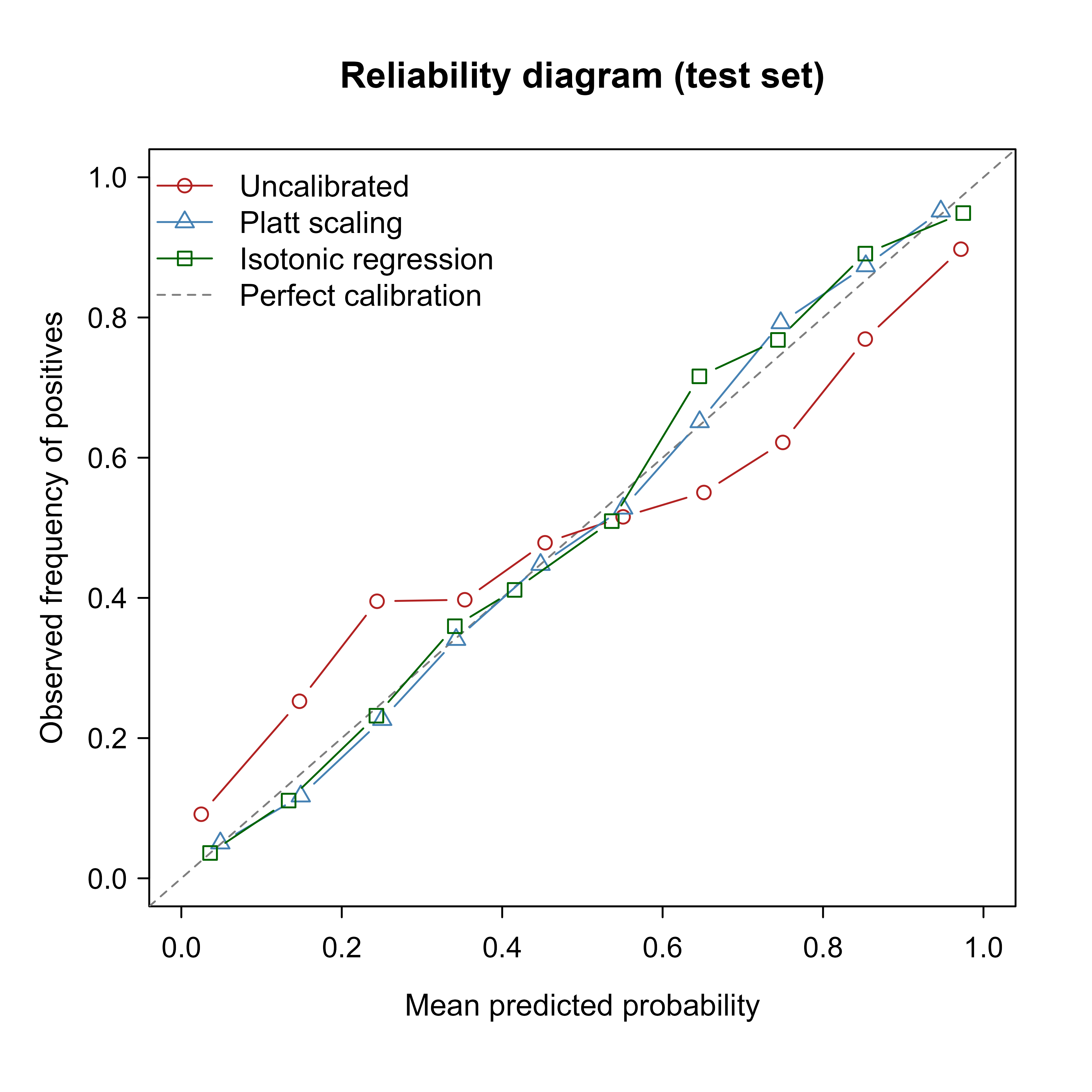
Figure 86.1 shows the uncalibrated curve sagging below the diagonal across the middle of the range: when the model says 0.8, positives actually appear less often than 80% of the time. After recalibration both curves snap back toward the diagonal, matching the drop in ECE from Table 86.2.
Note
We applied Platt scaling to the model’s log-odds and isotonic regression to its probabilities. Either method can take either input; what matters is that the input is a monotone function of the score and that the map is fit on held-out data. Here both happened to work well because the injected distortion is smooth and monotone.
86.7 Practical guidance and pitfalls
A few habits separate trustworthy calibration from theater.
Always hold out a calibration set. The single most common mistake is fitting the calibrator on training data. The model’s training-set probabilities are optimistically honest, so the calibrator learns a near-identity map and does nothing in production. If data are scarce, use cross-validated calibration: split into folds, fit the model on the rest, calibrate on the held-out fold, and average the maps. This is the idea behind scikit-learn’s CalibratedClassifierCV and is worth replicating.
Recalibration cannot create discrimination it never had. A monotone map repairs the numbers but preserves the ranking. If your model cannot tell positives from negatives (AUC near 0.5), no amount of calibration will help; you need a better model, not a better calibrator. Calibration is the last mile, not the road.
Match the method to the data budget. With a few hundred calibration points, prefer temperature or Platt scaling; their handful of parameters resist overfitting. With several thousand, isotonic regression can capture distortions the parametric methods miss. When in doubt, the more constrained method generalizes better.
Beware the binning illusion in ECE. Because ECE depends on the number and placement of bins, you can make a model look better or worse by retuning the bins. Fix the binning scheme up front, compare models under identical bins, and report the scheme. For a binning-free alternative, consider kernel-smoothed calibration estimates or the integrated calibration index.
Multiclass is harder than it looks. For \(K > 2\) classes the natural extension is to calibrate the full probability vector, but the common shortcut of calibrating each class one-versus-rest does not guarantee the calibrated probabilities sum to one, requiring renormalization. Temperature scaling sidesteps this neatly because it rescales all logits at once and the softmax renormalizes automatically, which is part of why it is the default for deep networks.
Calibration drifts. A model calibrated at deployment can drift as the population shifts. Monitor calibration in production the way you monitor accuracy, and be prepared to refit the calibration map (which is cheap) far more often than you retrain the model (which is expensive).
Warning
Do not report calibration on the same data you used to fit the calibrator, and do not report it on the data you tuned bins against. The clean protocol is three disjoint sets, train, calibrate, test, with all final metrics on the test set, exactly as in the demonstration above.
86.8 Temperature scaling in a deep network (illustrative)
For completeness, here is the canonical temperature-scaling recipe for a neural network, expressed in PyTorch-style pseudocode. It is shown rather than run, since the book’s executable examples are in R, but the logic transfers directly: collect the logits and labels on a validation set, then optimize a single scalar \(T\) to minimize negative log-likelihood.
Show code
import torch
import torch.nn as nn
import torch.optim as optim

# `logits` : (N, K) tensor of pre-softmax outputs on a held-out validation set
# `labels` : (N,)   tensor of integer class labels

class TemperatureScaler(nn.Module):
    def __init__(self):
        super().__init__()
        # A single positive scalar, initialized at 1.0 (no change).
        self.temperature = nn.Parameter(torch.ones(1) * 1.0)

    def forward(self, logits):
        return logits / self.temperature

def fit_temperature(logits, labels, max_iter=50):
    scaler = TemperatureScaler()
    nll = nn.CrossEntropyLoss()
    # LBFGS is the standard choice: one scalar, smooth objective.
    optimizer = optim.LBFGS([scaler.temperature], lr=0.01, max_iter=max_iter)

    def closure():
        optimizer.zero_grad()
        loss = nll(scaler(logits), labels)
        loss.backward()
        return loss

    optimizer.step(closure)
    return scaler.temperature.detach()

# After fitting, calibrated probabilities are softmax(logits / T).
T = fit_temperature(logits, labels)
calibrated_probs = torch.softmax(logits / T, dim=1)
The single learned scalar T is then frozen and applied to every future prediction. Because it does not change which logit is largest, the network’s accuracy is identical before and after; only the confidence is corrected.
86.9 Further reading
For the foundational treatment of calibration as a property of probabilistic forecasts and the Brier-score decomposition, see Murphy (1973) and the broader scoring-rules framework in Gneiting and Raftery (2007). Platt (1999) introduced sigmoid (Platt) scaling for support vector machines. Zadrozny and Elkan (2001, 2002) developed and analyzed binning and isotonic-regression calibration for decision trees and naive Bayes, and Niculescu-Mizil and Caruana (2005) gave the influential empirical comparison of calibration across model families that explains the over- and under-confidence patterns described here. For modern deep networks, Guo, Pleiss, Sun, and Weinberger (2017) is the standard reference on over-confidence and temperature scaling, and Kull and colleagues (2019) extend the parametric approach with Dirichlet calibration for the multiclass case. Naeini, Cooper, and Hauskrecht (2015) formalized the expected calibration error used throughout this chapter.
This is why the recalibration methods below are all monotone functions of the original score. Platt scaling is a logistic curve, isotonic regression is a non-decreasing step function, and temperature scaling is a monotone reshaping of the logits. None of them reorders cases, so AUC is preserved up to ties.↩︎
Pool adjacent violators sweeps through the score-sorted labels, and whenever the running fitted values would decrease, it pools the offending neighbors into a single block set to their average. The result is the unique non-decreasing least-squares fit, computable in linear time.↩︎