A child who has seen a single picture of a zebra can recognize zebras for the rest of their life. Show them one example, point, say the word once, and they generalize to new poses, lighting, and backgrounds. They can do something stranger still: tell them in words that a zebra is “a horse with black and white stripes,” show them no picture at all, and they will still pick the zebra out of a lineup. Standard supervised learning, the workhorse of the supervised parts of this book, does neither of these things gracefully. It expects hundreds or thousands of labeled examples per class, and it can only predict classes it saw during training.
This chapter is about the two regimes that close that gap. Few-shot learning asks a model to recognize a new concept from a handful of labeled examples, sometimes a single one. Zero-shot learning asks it to recognize a class it has never seen any example of, using only a description: a list of attributes, a word embedding, or a sentence of text. Both matter in practice because labels are expensive and the world keeps producing new categories. A new product appears in a catalog with three photos. A rare disease subtype shows up in five patients. A fraud pattern emerges with a dozen confirmed cases. Waiting to collect ten thousand examples is not an option, and sometimes there will never be ten thousand examples to collect.
The intuition that unifies both regimes is the same one the child used: do not memorize pixels, learn a space in which similarity is meaningful, then classify by comparison. If “looks alike” and “is the same kind of thing” line up in that space, you can recognize a new class from one example (compare to the example) or from a description (compare to the description). The work is in building the space; classification afterward is just measuring distance.
Intuition
Standard classifiers learn a fixed set of decision boundaries, one per known class. Few-shot and zero-shot methods instead learn a representation plus a comparison rule, so that a brand new class can be slotted in at test time by placing its examples or its description into the same space and asking what is nearby.
This chapter develops the formal setup (\(N\)-way \(K\)-shot episodes, support and query sets), explains why ordinary training collapses with few examples, walks through the metric-based and optimization-based families (cross-referencing the meta-learning chapter (Chapter 53) for MAML), then turns to zero-shot learning through attributes and semantic embeddings, the way modern vision-language models such as CLIP and large language models perform zero-shot classification, and the practical traps (generalized zero-shot bias and the hubness problem). Two runnable base-R demonstrations anchor the ideas: a nearest-centroid few-shot classifier evaluated across shot counts, and an attribute-based zero-shot classifier that recognizes a class for which it has seen no training examples at all.
52.1 Why standard training fails with few examples
Fit a logistic regression or a neural network to one labeled example per class and the result is not just weak, it is structurally broken. To see why, consider what a parametric classifier is doing: estimating decision-boundary parameters from data. With \(p\) features and one example per class, the system is wildly underdetermined. There are infinitely many boundaries that separate the training points perfectly, and ordinary empirical risk minimization has no principled way to choose among them. Whatever it lands on is dictated by the random initialization and the regularizer, not by anything generalizable about the classes.
Formally, if we minimize empirical risk \[
\hat{R}(\theta) \;=\; \frac{1}{n} \sum_{i=1}^{n} \ell\!\left(f_\theta(x_i),\, y_i\right)
\] over a flexible family \(f_\theta\), the gap between empirical risk and true risk \(R(\theta) = \mathbb{E}_{(x,y)}[\ell(f_\theta(x), y)]\) scales, very roughly, with model capacity divided by \(\sqrt{n}\). Drive \(n\) down to a handful and that gap explodes: the model memorizes the few points and generalizes by accident. Regularization helps but cannot manufacture information that the data does not contain.
Key idea
With few examples the bottleneck is not the optimizer or the architecture, it is information. The only escape is to inject information from outside the few labeled points: from related tasks (few-shot meta-learning) or from side information about the classes themselves (zero-shot learning).
Both regimes in this chapter are, at heart, strategies for importing that outside information. Few-shot learning borrows it from a large collection of other classification tasks that resemble the target. Zero-shot learning borrows it from a description of each class expressed in a shared semantic space. Neither violates the no-free-lunch principle: the information is paid for, just somewhere other than the few labels in front of you.
52.2 The few-shot setup: episodes, support, and query
The vocabulary of few-shot learning is borrowed from the meta-learning literature. We assume a distribution over tasks\(p(\mathcal{T})\), where each task is a small classification problem in its own right. A single task, also called an episode, draws \(N\) classes and provides two disjoint sets:
a support set \(\mathcal{S} = \{(x_j, y_j)\}_{j=1}^{NK}\) with \(K\) labeled examples per class, so \(NK\) examples total, and
a query set \(\mathcal{Q} = \{(x_j^\*, y_j^\*)\}\) drawn from the same \(N\) classes, used to measure how well the model classified after seeing only \(\mathcal{S}\).
This is the \(N\)-way \(K\)-shot protocol: \(N\) classes to choose among, \(K\) labeled examples per class.1 A 5-way 1-shot task is five classes with a single labeled example each; a 5-way 5-shot task gives five examples each. The decisive constraint is that the classes differ from episode to episode, and the classes used to evaluate are disjoint from the classes used to train the representation. A model cannot succeed by memorizing a fixed label set; it must learn a rule for adapting to whatever classes an episode presents.
Note
The support/query split inside one task is what separates few-shot learning from ordinary supervised learning. The support set is the “training data the model may adapt on” and the query set is the “test data,” but both live inside a single episode, and we repeat this miniature train/test split across thousands of episodes. Performance is reported as average query accuracy over many held-out episodes.
52.2.1 The episodic objective
We want a model that, given any support set, produces a good classifier for that episode’s query set. Write the model’s prediction on a query point \(x^\*\) as \(f_\theta(x^\* \mid \mathcal{S})\), explicitly conditioned on the support set. The meta-objective averages the query loss over the task distribution: \[
\min_\theta \;\; \mathbb{E}_{\mathcal{T} \sim p(\mathcal{T})}\;
\mathbb{E}_{(\mathcal{S}, \mathcal{Q}) \sim \mathcal{T}}
\left[\; \frac{1}{|\mathcal{Q}|} \sum_{(x^\*, y^\*) \in \mathcal{Q}} \ell\!\left(f_\theta(x^\* \mid \mathcal{S}),\, y^\*\right) \right].
\] Training mirrors testing: each gradient step samples a fresh episode, adapts on its support set, and is scored on its query set. This alignment between training and deployment conditions is the core trick. The families below differ only in how \(f_\theta(\cdot \mid \mathcal{S})\) turns a support set into a classifier.
52.3 Metric-based methods: prototypical networks
The simplest and most durable idea is metric-based. Learn an embedding \(g_\theta : \mathcal{X} \to \mathbb{R}^d\) that maps inputs into a feature space, then classify a query point by its distance to each class in that space. Prototypical networks (Snell, Swersky, and Zemel, 2017) make this concrete: represent each class by the mean of its support embeddings, the prototype, and assign a query point to the nearest prototype.
For class \(c\) with support examples \(\mathcal{S}_c\), the prototype is \[
\mu_c \;=\; \frac{1}{|\mathcal{S}_c|} \sum_{(x, y) \in \mathcal{S}_c} g_\theta(x).
\] A query point \(x^\*\) is scored by negative squared Euclidean distance to each prototype, turned into a distribution over classes by a softmax: \[
p_\theta(y = c \mid x^\*) \;=\; \frac{\exp\!\left(-\lVert g_\theta(x^\*) - \mu_c \rVert^2\right)}{\sum_{c'} \exp\!\left(-\lVert g_\theta(x^\*) - \mu_{c'} \rVert^2\right)}.
\] Training minimizes the negative log-likelihood of the true query labels under this distribution, backpropagating through the embedding \(g_\theta\). At test time, on a brand new episode with never-before-seen classes, you simply compute prototypes from the support set and classify queries by nearest prototype: no gradient steps, no retraining.
Intuition
A prototype is the “average look” of a class given its few examples. Classifying by nearest prototype says: a query is whatever class it most resembles on average. If the embedding has been shaped so that same-class points cluster, one or a few examples are enough to locate the cluster center.
There is a clean probabilistic reading. With squared-Euclidean distance, the softmax above is exactly the posterior of a Gaussian mixture in which every class shares an identity covariance and the prototype is the class mean. Prototypical networks are, in the embedding space, a one-nearest-centroid classifier (equivalently, linear discriminant analysis (Chapter 20) with tied isotropic covariance). Their power comes entirely from learning an embedding \(g_\theta\), across many episodes, in which that simple decision rule works. Relatives in this family include matching networks (Vinyals et al., 2016), which use an attention-weighted nearest neighbor, and relation networks (Sung et al., 2018), which learn the comparison metric itself (Chapter 63) rather than fixing it to Euclidean distance.
52.3.1 Derivation: why squared Euclidean distance gives a linear classifier
The claim that the prototype softmax is a Gaussian-mixture posterior, and that it is linear in the embedding, is worth deriving because it explains both the appeal and the limits of the method. Suppose each class \(c\) generates embeddings from \(\mathcal{N}(\mu_c, \sigma^2 I)\) with a shared isotropic covariance and equal priors \(\pi_c = 1/N\). Let \(z = g_\theta(x^\*)\). By Bayes’ rule the posterior is \[
p(y = c \mid z) \;=\; \frac{\pi_c \, \exp\!\left(-\tfrac{1}{2\sigma^2}\lVert z - \mu_c \rVert^2\right)}{\sum_{c'} \pi_{c'} \, \exp\!\left(-\tfrac{1}{2\sigma^2}\lVert z - \mu_{c'} \rVert^2\right)} .
\] Expand the squared norm in the exponent, \(\lVert z - \mu_c \rVert^2 = \lVert z \rVert^2 - 2\,\mu_c^\top z + \lVert \mu_c \rVert^2\). The term \(\lVert z \rVert^2\) is the same for every class, so it cancels between numerator and denominator. Absorbing it and the (equal) priors leaves \[
p(y = c \mid z) \;=\; \frac{\exp\!\left(w_c^\top z + b_c\right)}{\sum_{c'} \exp\!\left(w_{c'}^\top z + b_{c'}\right)},
\qquad
w_c = \frac{1}{\sigma^2}\mu_c, \quad
b_c = -\frac{1}{2\sigma^2}\lVert \mu_c \rVert^2 .
\tag{52.1}\] Equation Equation 52.1 is an ordinary softmax (multinomial logistic) classifier whose weight vector for class \(c\) is the prototype itself, scaled by \(1/\sigma^2\), and whose bias is set by the prototype norm. Two consequences follow. First, prototypical networks impose a linear decision rule in embedding space; all nonlinearity must be carried by \(g_\theta\), which is why a poor embedding cannot be rescued by the classifier. Second, the temperature is the noise scale \(\sigma^2\): the chapter’s softmax fixes \(\sigma^2 = 1/2\) implicitly by writing \(\exp(-\lVert z - \mu_c\rVert^2)\), but in practice a learnable temperature \(\tau\) in \(\exp(-\lVert z - \mu_c\rVert^2/\tau)\) materially affects calibration and is worth tuning. Using cosine distance instead of squared Euclidean breaks this exact equivalence (the \(\lVert z\rVert^2\) term no longer cancels cleanly) but is often preferred empirically because it removes embedding-norm effects.
52.3.2 Prototype variance and the \(1/K\) rate
The diminishing returns visible in Figure 52.1 have a precise cause. The prototype \(\mu_c = \frac{1}{K}\sum_{j=1}^K z_j\) is a sample mean of \(K\) embeddings, so if the true class-conditional embedding has mean \(\mu_c^\star\) and covariance \(\Sigma_c\), then \[
\mathbb{E}[\mu_c] = \mu_c^\star, \qquad
\operatorname{Cov}(\mu_c) = \frac{1}{K}\Sigma_c .
\tag{52.2}\] The prototype is unbiased for the true class center, and its estimation variance falls as \(1/K\), so the standard error of each prototype coordinate shrinks like \(1/\sqrt{K}\). Because the decision boundary between two classes is the perpendicular bisector of their prototypes, boundary jitter inherits this \(1/\sqrt{K}\) rate, and the resulting error rate above its asymptote (the Bayes rate for the fixed embedding) decays on the same order. This is why the curve gains most in the first few shots and then flattens: going from one shot to two halves the prototype variance, but going from ten to twenty cuts it only by a further factor of two off an already small base. It also explains why one-shot is the genuinely hard regime, the prototype is a single noisy point with no averaging at all.
52.4 Optimization-based methods and a pointer to MAML
A different family treats few-shot learning as learning an initialization (or an optimizer) from which a few gradient steps on the support set yield a good classifier. The flagship is Model-Agnostic Meta-Learning, MAML (Finn, Abbeel, and Levine, 2017). MAML learns parameters \(\theta\) such that, for a new task, a small number of gradient steps on the support loss produces task-adapted parameters \(\theta'\) that perform well on the query set. The inner loop adapts; the outer loop optimizes the initialization so that adaptation is fast.
Because the meta-learning chapter (Chapter 53) develops MAML, its inner/outer-loop objective, and the second-order gradient that makes it work in full, this chapter does not repeat that derivation. See that chapter for the optimization-based view; the takeaway here is the contrast in Table 52.1.
Show code
fam<-data.frame( Family =c("Metric-based", "Optimization-based", "Fine-tuning / transfer", "In-context (LLM)"), `What is learned` =c("An embedding + fixed distance rule","An initialization adapted by gradient steps","Pretrained weights, then task-specific tuning","Nothing at test time; conditions on prompt"), `Test-time adaptation` =c("None (compute prototypes)","A few gradient steps on support","Many gradient steps on the new task","None (examples placed in the prompt)"), Example =c("Prototypical nets", "MAML", "ImageNet pretrain + tune", "GPT-style few-shot prompting"), check.names =FALSE)knitr::kable(fam, caption ="Few-shot learning families compared by what is learned and how (if at all) the model adapts at test time.")
Table 52.1: Few-shot learning families compared by what is learned and how (if at all) the model adapts at test time.
Family
What is learned
Test-time adaptation
Example
Metric-based
An embedding + fixed distance rule
None (compute prototypes)
Prototypical nets
Optimization-based
An initialization adapted by gradient steps
A few gradient steps on support
MAML
Fine-tuning / transfer
Pretrained weights, then task-specific tuning
Many gradient steps on the new task
ImageNet pretrain + tune
In-context (LLM)
Nothing at test time; conditions on prompt
None (examples placed in the prompt)
GPT-style few-shot prompting
Table 52.1 contrasts the families. Metric-based methods are attractive in practice because they need no test-time optimization: adding a new class is as cheap as embedding its support examples and storing a prototype. Optimization-based methods are more flexible but heavier, and fine-tuning sits at the data-hungry end. In-context learning with large language models is, in effect, metric-and-optimization-free adaptation whose “training across tasks” happened implicitly during pretraining.
52.5 A runnable few-shot demonstration: nearest-centroid classifier
The metric-based recipe is small enough to implement and study in base R, with no deep network required. We simulate a world of many classes, each a Gaussian blob in feature space, with a fixed (here, identity) embedding standing in for a learned \(g_\theta\). Each episode samples \(N\) fresh classes, draws \(K\) support points and some query points per class, builds prototypes, and classifies queries by nearest prototype. Averaging query accuracy over many episodes estimates expected few-shot performance, and sweeping \(K\) shows how accuracy climbs with shots.
Show code
set.seed(1301)# A "world" of many latent classes. Each class is a Gaussian blob whose mean is# a random point in d-dimensional space; the spread sigma controls difficulty.make_world<-function(n_classes=50, d=20, spread=2.0, sigma=1.0){centers<-matrix(rnorm(n_classes*d, sd =spread), nrow =n_classes, ncol =d)list(centers =centers, d =d, sigma =sigma, n_classes =n_classes)}# Draw `n` points from a given class (its blob). The identity embedding here# stands in for a learned embedding g_theta; in a real system g_theta is trained.draw_points<-function(world, class_id, n){mu<-world$centers[class_id, ]matrix(rnorm(n*world$d, mean =rep(mu, each =n), sd =world$sigma), nrow =n, ncol =world$d)}# One N-way K-shot episode: sample N classes, K support + Q query points each,# build prototypes (class means), classify queries by nearest prototype.run_episode<-function(world, N=5, K=1, Q=15){classes<-sample(world$n_classes, N)protos<-matrix(0, nrow =N, ncol =world$d)q_x<-matrix(0, nrow =N*Q, ncol =world$d)q_y<-integer(N*Q)for(iinseq_len(N)){s<-draw_points(world, classes[i], K)protos[i, ]<-colMeans(s)# prototype = mean support embeddingrows<-((i-1)*Q+1):(i*Q)q_x[rows, ]<-draw_points(world, classes[i], Q)q_y[rows]<-i}# Squared Euclidean distance from each query to each prototype, nearest wins.d2<-outer(rowSums(q_x^2), rowSums(protos^2), "+")-2*q_x%*%t(protos)pred<-max.col(-d2, ties.method ="first")mean(pred==q_y)}# Average query accuracy over many episodes for a given (N, K).few_shot_accuracy<-function(world, N=5, K=1, Q=15, episodes=400){mean(replicate(episodes, run_episode(world, N =N, K =K, Q =Q)))}
With the machinery in place we sweep the number of shots \(K\) for a 5-way problem and record accuracy.
Show code
world<-make_world(n_classes =50, d =30, spread =1.0, sigma =2.5)shots<-c(1, 2, 5, 10, 20)acc<-sapply(shots, function(k)few_shot_accuracy(world, N =5, K =k, episodes =400))sweep_tbl<-data.frame( Shots =shots, Accuracy =round(acc, 3), `Error rate` =round(1-acc, 3), check.names =FALSE)
Show code
knitr::kable(sweep_tbl, caption ="Mean 5-way query accuracy of the nearest-centroid few-shot classifier as the number of support examples per class (shots) increases, averaged over 400 simulated episodes.")
Table 52.2: Mean 5-way query accuracy of the nearest-centroid few-shot classifier as the number of support examples per class (shots) increases, averaged over 400 simulated episodes.
Shots
Accuracy
Error rate
1
0.369
0.631
2
0.454
0.546
5
0.584
0.416
10
0.663
0.337
20
0.718
0.282
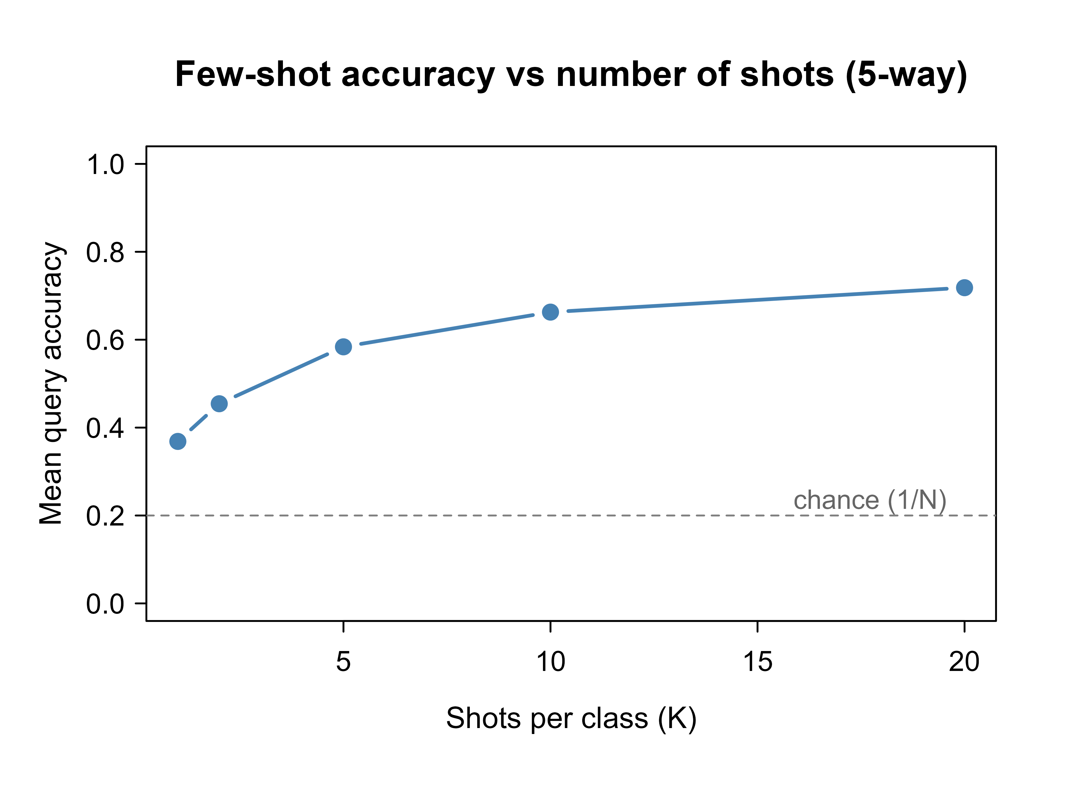
Table 52.2 reports the numbers and Figure 52.1 plots them. Two things are visible. First, even 1-shot accuracy is far above the 20% chance level of a 5-way problem, because the learned (here, simulated) embedding already separates classes. Second, accuracy rises with shots but with diminishing returns: most of the benefit arrives in the first few examples, because averaging more support points mainly reduces the variance of the prototype estimate, and that variance shrinks like \(1/K\).
Show code
plot(shots, acc, type ="b", pch =19, lwd =2, col ="steelblue", xlab ="Shots per class (K)", ylab ="Mean query accuracy", main ="Few-shot accuracy vs number of shots (5-way)", ylim =c(0, 1))abline(h =1/5, lty =2, col ="grey50")text(max(shots), 1/5+0.03, "chance (1/N)", pos =2, col ="grey40", cex =0.9)
Figure 52.1: 5-way nearest-centroid accuracy versus number of shots per class. Accuracy climbs steeply from 1-shot then flattens, the diminishing-returns pattern typical of few-shot learning. The dashed line marks 20% chance accuracy for a 5-way task.
Figure 52.1 is the empirical signature of few-shot learning: large gains from the first example, then flattening. The same curve shape appears with real learned embeddings; the difference is only how high the curve starts, which is governed by how well the embedding separates unseen classes.
The \(1/K\) variance law of Equation 52.2 is easy to confirm directly: estimate the trace of the prototype covariance by Monte Carlo for a range of \(K\) and check that it scales like \(1/K\).
Show code
set.seed(1301)mu_star<-world$centers[1, ]# a fixed true class centerproto_var<-function(K, reps=4000){protos<-t(replicate(reps, colMeans(draw_points(world, 1, K))))sum(apply(protos, 2, var))# trace of empirical Cov(prototype)}Ks<-c(1, 2, 5, 10, 20)tr<-sapply(Ks, proto_var)# Predicted: trace(Sigma)/K, with trace(Sigma) = d * sigma^2 for isotropic blobs.predicted<-world$d*world$sigma^2/Ksdata.frame(K =Ks, empirical =round(tr, 2), predicted =round(predicted, 2))#> K empirical predicted#> 1 1 187.98 187.50#> 2 2 94.40 93.75#> 3 5 37.44 37.50#> 4 10 18.82 18.75#> 5 20 9.33 9.38
The empirical prototype variance tracks the predicted \(d\sigma^2/K\) closely, confirming that more shots help only by averaging down a variance that already falls as \(1/K\).
When to use this
Reach for a metric-based few-shot approach when new classes arrive often, each with only a few labels, and you can afford to train a good embedding once on a large pool of related classes. Nearest-centroid classification on top of a strong pretrained embedding (an image encoder, a text encoder) is a remarkably hard baseline to beat, and it adds new classes with zero retraining.
52.6 Zero-shot learning: recognizing the unseen
Few-shot learning still needs at least one example. Zero-shot learning removes even that. The classes seen at test time, the unseen classes, have no labeled examples at all. The only thing connecting a test input to an unseen class is side information: a structured description of what each class is.
The setup splits the label space into seen classes \(\mathcal{Y}^s\) (with training images) and unseen classes \(\mathcal{Y}^u\) (with none), where \(\mathcal{Y}^s \cap \mathcal{Y}^u = \varnothing\). Every class \(c\), seen or unseen, comes with a semantic vector\(a_c \in \mathbb{R}^m\). This can be a hand-defined attribute vector (“has stripes,” “has four legs,” “lives in water,” each a 0/1 or a strength), a word embedding of the class name, or, in modern systems, a text encoding of a sentence describing the class. The semantic vectors are the bridge: they exist for unseen classes even though images do not.
Key idea
Zero-shot learning replaces “show me examples of the class” with “describe the class.” If you can place both the input and the class description into a shared space where matching things land near each other, you can recognize a class you have literally never seen, by matching its description to the input.
The classic recipe learns a compatibility function \(F(x, a)\) that scores how well an input \(x\) matches a semantic vector \(a\). A common linear form is \[
F(x, a) \;=\; \phi(x)^\top W\, a,
\] where \(\phi(x) \in \mathbb{R}^d\) is an input feature vector and \(W \in \mathbb{R}^{d \times m}\) is a learned mapping trained only on seen classes. At test time we predict the unseen class whose semantic vector scores highest: \[
\hat{y} \;=\; \arg\max_{c \,\in\, \mathcal{Y}^u} \; \phi(x)^\top W\, a_c .
\] Because \(W\) maps inputs into the semantic space (or aligns the two spaces), and because semantic vectors exist for unseen classes, the model can score classes it never trained on. The attribute structure is what carries information across the seen/unseen boundary: if “stripes” and “four legs” were learned from seen striped and four-legged animals, a never-seen zebra defined by those same attributes can be recognized.
52.6.1 Derivation: the closed-form compatibility solution (ESZSL)
The bilinear score \(F(x, a) = \phi(x)^\top W a\) has a training objective with a closed-form solution, which is worth deriving because it shows exactly how seen-class supervision determines \(W\) and why ridge regularization is not optional here. Stack the \(n\) seen-class training features as rows of \(X \in \mathbb{R}^{n \times d}\), and let \(S \in \mathbb{R}^{s \times m}\) hold the semantic vectors of the \(s\) seen classes as rows. Encode labels as a one-hot matrix \(Y \in \{0,1\}^{n \times s}\). The model’s score matrix over training points and seen classes is \(X W S^\top\), and the simplest objective fits these scores to the labels under a squared loss with Frobenius regularization (this is the Embarrassingly Simple Zero-Shot Learning, ESZSL, formulation of Romera-Paredes and Torr, 2015): \[
\mathcal{L}(W) \;=\; \big\lVert X W S^\top - Y \big\rVert_F^2
\;+\; \gamma \lVert X W \rVert_F^2
\;+\; \lambda \lVert W S^\top \rVert_F^2
\;+\; \gamma\lambda \lVert W \rVert_F^2 .
\] The three penalties control, respectively, the projection of features into feature space, the projection of attributes into attribute space, and (via the cross term) the raw map. Keeping the single penalty \(\beta\lVert W\rVert_F^2\) for clarity and differentiating, with the Frobenius identity \(\nabla_W \lVert AWB - Y\rVert_F^2 = 2 A^\top(AWB - Y)B^\top\), gives \[
\nabla_W \mathcal{L} \;=\; 2 X^\top (X W S^\top - Y) S \;+\; 2\beta W \;=\; 0 .
\] Setting \(V = X^\top X\) and \(G = S^\top S\) and rearranging yields the Sylvester equation \(V W G + \beta W = X^\top Y S\). When the penalty is split as \(\lambda\) on the attribute side and \(\gamma\) on the feature side (the original ESZSL choice), the stationary condition separates into a clean product of two ridge inverses: \[
\hat{W} \;=\; \big(X^\top X + \lambda I_d\big)^{-1} X^\top Y\, S \big(S^\top S + \gamma I_m\big)^{-1} .
\tag{52.3}\] Equation Equation 52.3 is a two-sided ridge regression: \((X^\top X + \lambda I)^{-1} X^\top\) is the usual feature-side ridge solution, \(S(S^\top S + \gamma I)^{-1}\) is a ridge-regularized pseudoinverse on the semantic side, and \(Y\) bridges them. The regularizers are essential, not cosmetic: \(S^\top S\) is \(m \times m\) but built from only \(s\) seen-class rows, so if \(s < m\) (fewer seen classes than attributes, the common case) it is singular and \(\gamma > 0\) is required to invert it at all. At test time the predicted unseen label is \(\hat y = \arg\max_{c \in \mathcal{Y}^u} \phi(x)^\top \hat W a_c\), and crucially \(a_c\) for unseen \(c\) never entered Equation 52.3; only seen semantics in \(S\) did. The chapter’s runnable demo fits a feature-to-attribute map \(W\) by per-attribute ridge regression, which is the special case \(S = I\) (each seen class supervises its own attribute targets directly) of this general bilinear form.
52.6.2 Vision-language models and LLMs do this at scale
Modern zero-shot classification is the same idea with learned, high-capacity encoders and natural-language side information. CLIP (Radford et al., 2021) trains an image encoder and a text encoder jointly on hundreds of millions of image-caption pairs, with a contrastive objective (Chapter 49) that pulls matching image-text pairs together and pushes mismatched pairs apart in a shared embedding space. To classify an image into arbitrary categories at test time, you write a text prompt for each candidate label (for example, “a photo of a {label}”), encode all prompts and the image, and pick the label whose text embedding has the highest cosine similarity to the image embedding. No category-specific training is needed; the labels can be anything expressible in words, including categories never named during training. Large language models perform zero-shot classification the same way in a purely textual modality: the input text and a description of each label are mapped into the model’s representation space, and the most compatible label is chosen, often simply by asking the model to name it.
Note
CLIP-style zero-shot is exactly the compatibility-function recipe with \(\phi\) an image encoder, the semantic vector \(a_c\) a text embedding of the label, and the score a cosine similarity. The conceptual content is identical to the attribute model below; only the encoders and the scale of training data differ.
The contrastive objective that produces the shared space is worth writing precisely, because it is what guarantees the cosine score is meaningful at test time. Given a batch of \(B\) image-text pairs, let \(u_i = f(\text{image}_i)/\lVert f(\text{image}_i)\rVert\) and \(v_j = g(\text{text}_j)/\lVert g(\text{text}_j)\rVert\) be the L2-normalized image and text embeddings, and let \(\tau\) be a learned temperature. CLIP minimizes a symmetric InfoNCE loss in which, for each image, the matching caption is the positive among all \(B\) captions as negatives, and vice versa: \[
\mathcal{L}
= -\frac{1}{2B}\sum_{i=1}^{B}
\left[
\log \frac{e^{\,u_i^\top v_i/\tau}}{\sum_{j=1}^{B} e^{\,u_i^\top v_j/\tau}}
\;+\;
\log \frac{e^{\,u_i^\top v_i/\tau}}{\sum_{j=1}^{B} e^{\,u_j^\top v_i/\tau}}
\right].
\tag{52.4}\] The first term is a \(B\)-way classification of which caption matches image \(i\); the second is the transposed problem. Minimizing Equation 52.4 drives \(u_i^\top v_i\) (matched cosine) above \(u_i^\top v_j\) (mismatched cosine) by a margin set by \(\tau\), which is exactly the property the zero-shot rule relies on: at test time the correct label text sits at higher cosine similarity to the image than any wrong label. Because the loss is over normalized embeddings and arbitrary text, the alignment learned on training captions transfers to label strings never seen during training, which is the source of the open-vocabulary behavior. See Chapter 49 for the InfoNCE bound on mutual information that this objective optimizes.
A minimal CLIP-style zero-shot classifier in PyTorch looks like the following. It needs the Python torch and clip stack, so it is shown for reference and not executed here.
Show code
import torch, clipfrom PIL import Imagedevice ="cuda"if torch.cuda.is_available() else"cpu"model, preprocess = clip.load("ViT-B/32", device=device)image = preprocess(Image.open("animal.jpg")).unsqueeze(0).to(device)labels = ["a photo of a zebra", "a photo of a horse", "a photo of a tiger"]text = clip.tokenize(labels).to(device)with torch.no_grad(): img_emb = model.encode_image(image) txt_emb = model.encode_text(text) img_emb /= img_emb.norm(dim=-1, keepdim=True) txt_emb /= txt_emb.norm(dim=-1, keepdim=True) sims = (img_emb @ txt_emb.T).softmax(dim=-1) # cosine similarity -> probsprint(labels[sims.argmax().item()]) # zero-shot prediction
52.7 A runnable zero-shot demonstration: attribute matching
To make the mechanism concrete and runnable in base R, we build a tiny attribute-based zero-shot classifier. Each class is defined by a binary attribute vector (does it have stripes? four legs? live in water?). We train a linear map from input features to attribute space using only seen classes, then classify inputs from an unseen class by matching predicted attributes to the unseen class’s known attribute vector. Crucially, the unseen class contributes no training examples; it contributes only its attribute description.
Show code
set.seed(1301)# Six animal-like classes described by 5 binary attributes. The unseen class# (zebra) is held out of training entirely; only its attribute vector is used.attr_names<-c("stripes", "four_legs", "aquatic", "large", "mane")classes<-rbind( horse =c(0, 1, 0, 1, 1), tiger =c(1, 1, 0, 1, 0), dolphin =c(0, 0, 1, 1, 0), frog =c(0, 1, 1, 0, 0), lion =c(0, 1, 0, 1, 1), zebra =c(1, 1, 0, 1, 1)# the unseen class)colnames(classes)<-attr_namesseen<-c("horse", "tiger", "dolphin", "frog", "lion")unseen<-"zebra"# Generate input "feature" vectors for a class. Features are a noisy linear# image of the attribute vector through a fixed random projection: this stands# in for a perception system whose features correlate with the attributes.m<-length(attr_names)d<-30proj<-matrix(rnorm(d*m), nrow =d, ncol =m)# attribute -> feature mapgen_features<-function(class_name, n, noise=0.6){a<-classes[class_name, ]base<-as.numeric(proj%*%a)matrix(rnorm(n*d, mean =rep(base, each =n), sd =noise), nrow =n, ncol =d)}
Now we generate training data from the seen classes only, fit a linear map from features to attributes by least squares (a separate regression per attribute), and use it to predict attributes for held-out inputs.
Show code
# Training set: only SEEN classes contribute examples.n_per<-80X_train<-do.call(rbind, lapply(seen, gen_features, n =n_per))A_train<-do.call(rbind, lapply(seen, function(cl)matrix(rep(classes[cl, ], n_per), nrow =n_per, byrow =TRUE)))# Learn W mapping features -> attribute space (ridge-stabilized least squares).lambda<-1e-2XtX<-t(X_train)%*%X_train+lambda*diag(d)W<-solve(XtX, t(X_train)%*%A_train)# d x mpredict_attributes<-function(X)X%*%W# rows: predicted attribute vectors# Zero-shot prediction: assign each input to the class (from a candidate set)# whose KNOWN attribute vector is closest to the predicted attributes.zero_shot_predict<-function(X, candidate_classes){pa<-predict_attributes(X)cand<-classes[candidate_classes, , drop =FALSE]d2<-outer(rowSums(pa^2), rowSums(cand^2), "+")-2*pa%*%t(cand)candidate_classes[max.col(-d2, ties.method ="first")]}
The real test is the unseen class. We generate inputs from zebra, a class that contributed nothing to training, and ask the model to classify them. In the strict zero-shot protocol the candidate set is the unseen classes only; we also report the harder generalized zero-shot protocol where seen and unseen classes compete together.
Show code
n_test<-200# Strict zero-shot: candidates restricted to unseen classes. With one unseen# class this is trivially correct, so we evaluate generalized zero-shot below# and also test that seen classes are still recognized.X_zebra<-gen_features("zebra", n_test)X_horse<-gen_features("horse", n_test)X_tiger<-gen_features("tiger", n_test)# Generalized zero-shot: seen AND unseen classes compete.all_classes<-rownames(classes)acc_zebra_gzsl<-mean(zero_shot_predict(X_zebra, all_classes)=="zebra")acc_horse_gzsl<-mean(zero_shot_predict(X_horse, all_classes)=="horse")acc_tiger_gzsl<-mean(zero_shot_predict(X_tiger, all_classes)=="tiger")# Strict zero-shot for zebra: candidates are unseen + a couple of distractors# the model could confuse it with (compete against seen classes individually).acc_zebra_strict<-mean(zero_shot_predict(X_zebra, c("zebra", "horse", "tiger"))=="zebra")zsl_tbl<-data.frame( `Test class` =c("zebra (unseen)", "zebra (unseen)", "horse (seen)", "tiger (seen)"), Protocol =c("strict (vs horse, tiger)", "generalized (all 6)","generalized (all 6)", "generalized (all 6)"), Accuracy =round(c(acc_zebra_strict, acc_zebra_gzsl,acc_horse_gzsl, acc_tiger_gzsl), 3), check.names =FALSE)
Show code
knitr::kable(zsl_tbl, caption ="Attribute-based zero-shot accuracy. The model is trained only on seen classes (horse, tiger, dolphin, frog, lion) yet recognizes the unseen zebra by matching predicted attributes to the zebra attribute vector. The generalized protocol, where seen and unseen classes compete together, is harder.")
Table 52.3: Attribute-based zero-shot accuracy. The model is trained only on seen classes (horse, tiger, dolphin, frog, lion) yet recognizes the unseen zebra by matching predicted attributes to the zebra attribute vector. The generalized protocol, where seen and unseen classes compete together, is harder.
Test class
Protocol
Accuracy
zebra (unseen)
strict (vs horse, tiger)
0.88
zebra (unseen)
generalized (all 6)
0.88
horse (seen)
generalized (all 6)
1.00
tiger (seen)
generalized (all 6)
1.00
Table 52.3 shows the payoff: the model classifies zebra inputs correctly despite never having trained on a single zebra, because the attribute vector (“striped, four-legged, large, maned”) is enough to distinguish it once the feature-to-attribute map has been learned from other animals. The harder generalized setting, where the model must also avoid mistaking zebras for the visually similar seen classes (horse and lion share four of five attributes with zebra), drops accuracy, which is exactly the bias we discuss next.
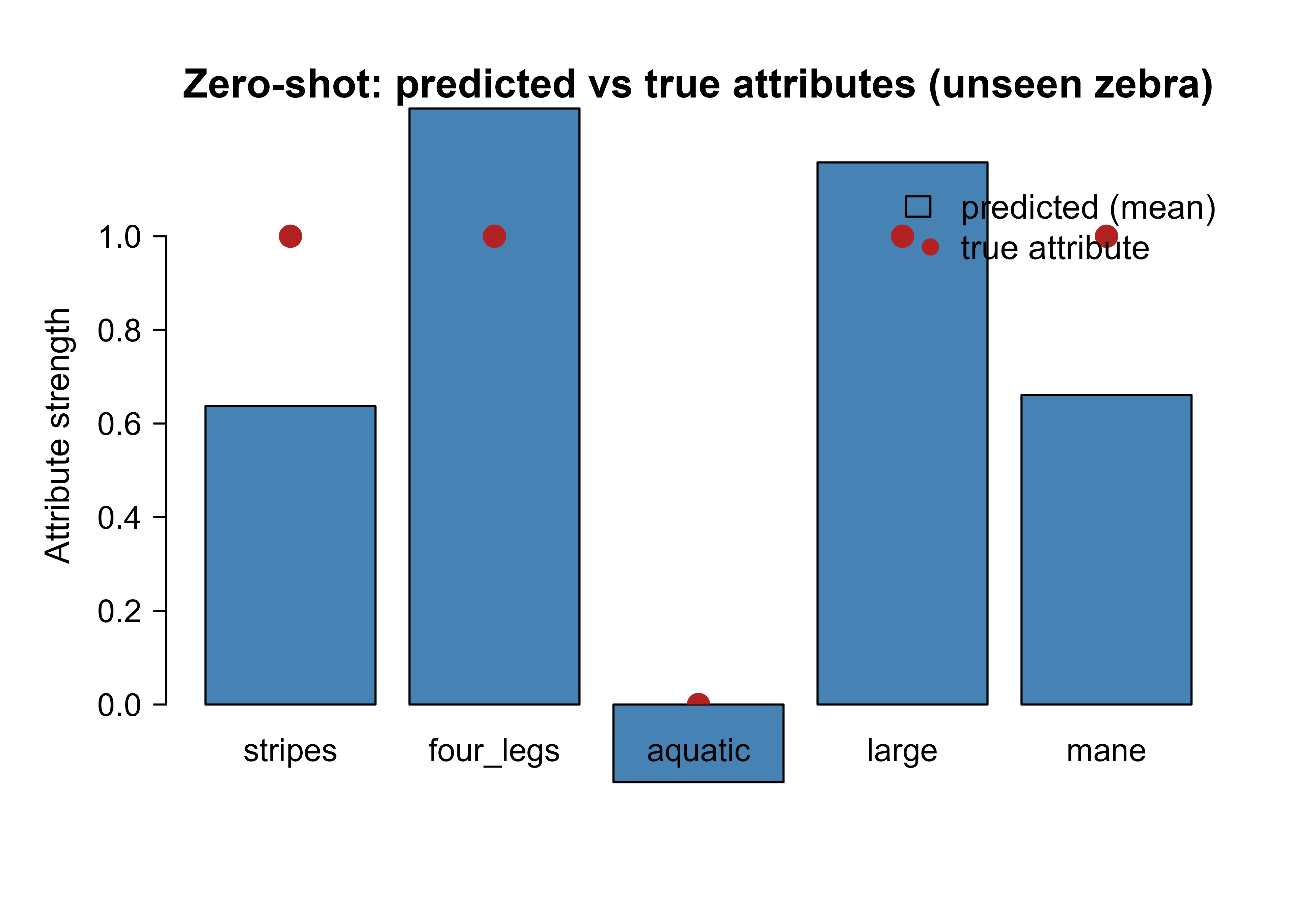
Figure 52.2 visualizes why the model can pull this off: the predicted attribute profile for zebra inputs lines up with the true zebra attributes, even though the predictions were produced by a map that never saw a zebra.
Show code
pa_zebra<-colMeans(predict_attributes(X_zebra))true_zebra<-classes["zebra", ]bp<-barplot(pa_zebra, names.arg =attr_names, col ="steelblue", ylim =c(0, 1.15), ylab ="Attribute strength", main ="Zero-shot: predicted vs true attributes (unseen zebra)")points(bp, true_zebra, pch =19, col ="firebrick", cex =1.4)legend("topright", legend =c("predicted (mean)", "true attribute"), fill =c("steelblue", NA), border =c("black", NA), pch =c(NA, 19), col =c(NA, "firebrick"), bty ="n")
Figure 52.2: Predicted versus true attribute vector for the unseen zebra class. Bars show the mean predicted attribute strength over 200 zebra inputs (from a map trained only on other animals); circles mark the true binary attributes. The predicted profile recovers the zebra’s defining attributes, which is what lets zero-shot matching succeed.
Figure 52.2 is the heart of the method made visible. Recognition of an unseen class reduces to predicting its attributes well and matching to the right description.
52.8 Generalized zero-shot and the hubness problem
Two failure modes deserve attention because they trip up nearly every newcomer.
The first is the bias toward seen classes in generalized zero-shot learning (GZSL). In the strict protocol, test inputs come only from unseen classes and candidates are restricted to unseen classes. That is unrealistic: in deployment you do not know in advance whether an input belongs to a seen or an unseen class, so both must compete. Because the compatibility map \(W\) was trained only on seen classes, it produces sharper, more confident scores for them, and unseen-class inputs get misrouted to seen classes. The honest metric for GZSL is therefore the harmonic mean of seen accuracy \(\text{Acc}_s\) and unseen accuracy \(\text{Acc}_u\): \[
H \;=\; \frac{2\, \text{Acc}_s\, \text{Acc}_u}{\text{Acc}_s + \text{Acc}_u}.
\] The harmonic mean punishes lopsided performance: a model that nails seen classes but fails on unseen ones (the typical bias) scores poorly, whereas a plain average would hide the problem. Calibration tricks (downweighting seen-class scores, calibrated stacking) exist precisely to combat this bias.
The standard fix, calibrated stacking (Chao et al., 2016), makes the bias an explicit, tunable scalar. Subtract a constant \(\gamma\) from the score of every seen class before taking the argmax over the union of seen and unseen labels: \[
\hat y \;=\; \arg\max_{c \,\in\, \mathcal{Y}^s \cup \mathcal{Y}^u}\;
\Big[\, F(x, a_c) \;-\; \gamma\, \mathbb{1}\{c \in \mathcal{Y}^s\} \,\Big].
\tag{52.5}\] At \(\gamma = -\infty\) every input is forced to a seen class (seen accuracy is maximized, unseen accuracy is zero); at \(\gamma = +\infty\) every input is forced to an unseen class (the reverse). Sweeping \(\gamma\) from one extreme to the other traces out a curve of \((\text{Acc}_u, \text{Acc}_s)\) pairs, the seen-unseen accuracy trade-off curve, and one reports its area or picks the \(\gamma\) that maximizes the harmonic mean \(H\) on a validation split. The single parameter Equation 52.5 exposes the bias directly: a large optimal \(\gamma\) is a quantitative confession that the raw compatibility scores favor seen classes.
Warning
Never report only strict zero-shot accuracy or a plain average of seen and unseen accuracy. Both flatter a model that has quietly collapsed onto the seen classes. Report the harmonic mean \(H\), and report seen and unseen accuracy separately so the imbalance is visible.
The second is the hubness problem. In high-dimensional embedding spaces, a few points (the “hubs”) become the nearest neighbor of an unusually large number of query points, regardless of true class. When you classify by nearest semantic vector, certain class vectors act as hubs and absorb predictions they should not, inflating their false-positive rate and starving other classes. Hubness is a geometric property of high-dimensional nearest-neighbor search, not a bug in any particular model, and it worsens as dimension grows. Common mitigations rescale or normalize the similarity scores: cross-domain similarity local scaling (CSLS), which subtracts each point’s average similarity to its neighbors before ranking, and simple ranking-based or normalized-similarity schemes that prevent any single vector from dominating.
Why hubness emerges is a concentration-of-measure effect. As dimension \(D\) grows, pairwise distances between independent points concentrate: the ratio of the spread of distances to their mean shrinks like \(1/\sqrt{D}\), so almost all points sit at nearly the same distance from any query. In that near-degenerate geometry, the small residual differences are dominated by each candidate’s distance to the data mean: points closer to the center of the cloud are systematically closer to everything, and therefore appear in many neighbor lists. The result is a skew in the \(k\)-occurrence distribution \(O_k(c)\), the number of query points for which class vector \(c\) ranks among the top \(k\), with a heavy right tail of hubs. This is precisely why raw nearest-semantic-vector zero-shot degrades as the embedding dimension rises.
CSLS corrects for the centrality bias by penalizing candidates that are everyone’s neighbor. Let \(\cos(x, a)\) be the cosine similarity and let \(r_k(a) = \frac{1}{k}\sum_{x' \in \mathcal{N}_k(a)} \cos(x', a)\) be the mean similarity of semantic vector \(a\) to its \(k\) nearest queries, with \(r_k(x)\) defined symmetrically for a query \(x\). The CSLS score is \[
\operatorname{CSLS}(x, a) \;=\; 2\cos(x, a) \;-\; r_k(x) \;-\; r_k(a) .
\tag{52.6}\] The subtracted term \(r_k(a)\) is large exactly for hubs, vectors that are highly similar to many points, so Equation 52.6 demotes them and lets non-hub classes win the matches they deserve. It reduces to plain cosine ranking when no vector is more central than another, so it costs nothing in the well-behaved case.
Intuition
Hubness is the “popular but indiscriminate” point. In a crowded high-dimensional space, some class description ends up suspiciously close to everything, so it wins matches it has no business winning. Fixes work by penalizing points that are everyone’s neighbor.
52.9 Practical guidance and pitfalls
A few hard-won points for applying these methods.
Embedding quality dominates everything. For both few-shot and zero-shot, the single biggest lever is the representation. A nearest-centroid classifier on top of a strong pretrained encoder routinely beats elaborate few-shot architectures on weak features. Spend your effort on the embedding (or use a good off-the-shelf one) before tuning the classifier.
Match training episodes to deployment. Few-shot accuracy is reported per \((N, K)\) regime, and it does not transfer cleanly across regimes. If deployment is 5-way 1-shot, evaluate (and ideally train) at 5-way 1-shot. Reporting 5-shot numbers and deploying at 1-shot overstates performance.
Be honest about side information in zero-shot. Zero-shot performance is bounded by how well the attributes or descriptions separate the classes. If two classes share identical attribute vectors, no zero-shot model can tell them apart, no matter how good the encoder. Audit the side information for collisions before blaming the model.
Use the right metric. As above: report the harmonic mean for GZSL, and watch for the seen-class bias and hubness. A suspiciously high overall accuracy in GZSL usually means the model is ignoring unseen classes.
Few-shot is not magic data. The information for few-shot generalization comes from the base classes used to train the embedding. If the base classes are unlike the novel classes, transfer fails. The method recognizes new instances of a familiar kind of variation, not arbitrary new structure.
When to use this
Use few-shot methods when new classes keep arriving with a few labels each and you have a large pool of related classes to learn an embedding from. Use zero-shot methods when you have rich, reliable descriptions of classes (attributes, text) and need to recognize classes for which collecting any labeled examples is impractical. When you have descriptions and a few examples, combine them: a few-shot classifier whose prototypes are initialized from semantic vectors often beats either alone.
52.10 Further reading
Snell, Swersky, and Zemel (2017) introduce prototypical networks, the metric-based method implemented in this chapter.
Vinyals, Blundell, Lillicrap, Kavukcuoglu, and Wierstra (2016) propose matching networks and articulate the episodic few-shot training protocol.
Sung, Yang, Zhang, Xiang, Torr, and Hospedales (2018) present relation networks, which learn the comparison metric rather than fixing it.
Finn, Abbeel, and Levine (2017) introduce MAML, the optimization-based meta-learner; see the Meta-Learning chapter of this book.
Lampert, Nickisch, and Harmeling (2009) establish attribute-based zero-shot classification, the basis of the attribute demonstration here.
Xian, Lampert, Schiele, and Akata (2019) give the standard generalized zero-shot evaluation protocol and the harmonic-mean metric.
Romera-Paredes and Torr (2015) derive the embarrassingly simple (ESZSL) closed-form bilinear compatibility solution used above.
Chao, Changpinyo, Gong, and Sha (2016) introduce calibrated stacking and the seen-unseen accuracy trade-off curve for generalized zero-shot learning.
Conneau, Lample, Ranzato, Denoyer, and Jegou (2018) introduce CSLS as a hubness-aware retrieval criterion.
Radford et al. (2021) present CLIP, the contrastive vision-language model behind modern zero-shot image classification.
Radovanovic, Nanopoulos, and Ivanovic (2010) analyze the hubness problem in high-dimensional nearest-neighbor spaces.
Wang, Yao, Kwok, and Ni (2020) survey few-shot learning methods and their taxonomy.
The word “shot” is one labeled example you are permitted to see for a class, and “\(N\)-way” counts the classes in the decision. A 5-way 1-shot task is a five-class problem with exactly one labeled example per class, evaluated on fresh query points from those same five classes.↩︎
Source Code
# Few-Shot and Zero-Shot Learning {#sec-few-shot-zero-shot}```{r}#| include: falsesource("_common.R")```A child who has seen a single picture of a zebra can recognize zebras for the rest of their life. Show them one example, point, say the word once, and they generalize to new poses, lighting, and backgrounds. They can do something stranger still: tell them in words that a zebra is "a horse with black and white stripes," show them no picture at all, and they will still pick the zebra out of a lineup. Standard supervised learning, the workhorse of the supervised parts of this book, does neither of these things gracefully. It expects hundreds or thousands of labeled examples per class, and it can only predict classes it saw during training.This chapter is about the two regimes that close that gap. *Few-shot learning* asks a model to recognize a new concept from a handful of labeled examples, sometimes a single one. *Zero-shot learning* asks it to recognize a class it has never seen any example of, using only a description: a list of attributes, a word embedding, or a sentence of text. Both matter in practice because labels are expensive and the world keeps producing new categories. A new product appears in a catalog with three photos. A rare disease subtype shows up in five patients. A fraud pattern emerges with a dozen confirmed cases. Waiting to collect ten thousand examples is not an option, and sometimes there will never be ten thousand examples to collect.The intuition that unifies both regimes is the same one the child used: do not memorize pixels, learn a *space* in which similarity is meaningful, then classify by comparison. If "looks alike" and "is the same kind of thing" line up in that space, you can recognize a new class from one example (compare to the example) or from a description (compare to the description). The work is in building the space; classification afterward is just measuring distance.::: {.callout-tip title="Intuition"}Standard classifiers learn a fixed set of decision boundaries, one per known class. Few-shot and zero-shot methods instead learn a *representation* plus a *comparison rule*, so that a brand new class can be slotted in at test time by placing its examples or its description into the same space and asking what is nearby.:::This chapter develops the formal setup ($N$-way $K$-shot episodes, support and query sets), explains why ordinary training collapses with few examples, walks through the metric-based and optimization-based families (cross-referencing the meta-learning chapter (@sec-meta-learning) for MAML), then turns to zero-shot learning through attributes and semantic embeddings, the way modern vision-language models such as CLIP and large language models perform zero-shot classification, and the practical traps (generalized zero-shot bias and the hubness problem). Two runnable base-R demonstrations anchor the ideas: a nearest-centroid few-shot classifier evaluated across shot counts, and an attribute-based zero-shot classifier that recognizes a class for which it has seen no training examples at all.## Why standard training fails with few examplesFit a logistic regression or a neural network to one labeled example per class and the result is not just weak, it is structurally broken. To see why, consider what a parametric classifier is doing: estimating decision-boundary parameters from data. With $p$ features and one example per class, the system is wildly underdetermined. There are infinitely many boundaries that separate the training points perfectly, and ordinary empirical risk minimization has no principled way to choose among them. Whatever it lands on is dictated by the random initialization and the regularizer, not by anything generalizable about the classes.Formally, if we minimize empirical risk$$\hat{R}(\theta) \;=\; \frac{1}{n} \sum_{i=1}^{n} \ell\!\left(f_\theta(x_i),\, y_i\right)$$over a flexible family $f_\theta$, the gap between empirical risk and true risk $R(\theta) = \mathbb{E}_{(x,y)}[\ell(f_\theta(x), y)]$ scales, very roughly, with model capacity divided by $\sqrt{n}$. Drive $n$ down to a handful and that gap explodes: the model memorizes the few points and generalizes by accident. Regularization helps but cannot manufacture information that the data does not contain.::: {.callout-important title="Key idea"}With few examples the bottleneck is not the optimizer or the architecture, it is information. The only escape is to inject information from *outside* the few labeled points: from related tasks (few-shot meta-learning) or from side information about the classes themselves (zero-shot learning).:::Both regimes in this chapter are, at heart, strategies for importing that outside information. Few-shot learning borrows it from a large collection of *other* classification tasks that resemble the target. Zero-shot learning borrows it from a description of each class expressed in a shared semantic space. Neither violates the no-free-lunch principle: the information is paid for, just somewhere other than the few labels in front of you.## The few-shot setup: episodes, support, and queryThe vocabulary of few-shot learning is borrowed from the meta-learning literature. We assume a distribution over *tasks* $p(\mathcal{T})$, where each task is a small classification problem in its own right. A single task, also called an *episode*, draws $N$ classes and provides two disjoint sets:- a support set $\mathcal{S} = \{(x_j, y_j)\}_{j=1}^{NK}$ with $K$ labeled examples per class, so $NK$ examples total, and- a query set $\mathcal{Q} = \{(x_j^\*, y_j^\*)\}$ drawn from the same $N$ classes, used to measure how well the model classified after seeing only $\mathcal{S}$.This is the $N$-way $K$-shot protocol: $N$ classes to choose among, $K$ labeled examples per class.^[The word "shot" is one labeled example you are permitted to see for a class, and "$N$-way" counts the classes in the decision. A 5-way 1-shot task is a five-class problem with exactly one labeled example per class, evaluated on fresh query points from those same five classes.] A 5-way 1-shot task is five classes with a single labeled example each; a 5-way 5-shot task gives five examples each. The decisive constraint is that the classes differ from episode to episode, and the classes used to evaluate are disjoint from the classes used to train the representation. A model cannot succeed by memorizing a fixed label set; it must learn a *rule for adapting* to whatever classes an episode presents.::: {.callout-note}The support/query split inside one task is what separates few-shot learning from ordinary supervised learning. The support set is the "training data the model may adapt on" and the query set is the "test data," but both live inside a single episode, and we repeat this miniature train/test split across thousands of episodes. Performance is reported as average query accuracy over many held-out episodes.:::### The episodic objectiveWe want a model that, given any support set, produces a good classifier for that episode's query set. Write the model's prediction on a query point $x^\*$ as $f_\theta(x^\* \mid \mathcal{S})$, explicitly conditioned on the support set. The meta-objective averages the query loss over the task distribution:$$\min_\theta \;\; \mathbb{E}_{\mathcal{T} \sim p(\mathcal{T})}\;\mathbb{E}_{(\mathcal{S}, \mathcal{Q}) \sim \mathcal{T}}\left[\; \frac{1}{|\mathcal{Q}|} \sum_{(x^\*, y^\*) \in \mathcal{Q}} \ell\!\left(f_\theta(x^\* \mid \mathcal{S}),\, y^\*\right) \right].$$Training mirrors testing: each gradient step samples a fresh episode, adapts on its support set, and is scored on its query set. This alignment between training and deployment conditions is the core trick. The families below differ only in how $f_\theta(\cdot \mid \mathcal{S})$ turns a support set into a classifier.## Metric-based methods: prototypical networksThe simplest and most durable idea is metric-based. Learn an embedding $g_\theta : \mathcal{X} \to \mathbb{R}^d$ that maps inputs into a feature space, then classify a query point by its distance to each class in that space. *Prototypical networks* (Snell, Swersky, and Zemel, 2017) make this concrete: represent each class by the mean of its support embeddings, the *prototype*, and assign a query point to the nearest prototype.For class $c$ with support examples $\mathcal{S}_c$, the prototype is$$\mu_c \;=\; \frac{1}{|\mathcal{S}_c|} \sum_{(x, y) \in \mathcal{S}_c} g_\theta(x).$$A query point $x^\*$ is scored by negative squared Euclidean distance to each prototype, turned into a distribution over classes by a softmax:$$p_\theta(y = c \mid x^\*) \;=\; \frac{\exp\!\left(-\lVert g_\theta(x^\*) - \mu_c \rVert^2\right)}{\sum_{c'} \exp\!\left(-\lVert g_\theta(x^\*) - \mu_{c'} \rVert^2\right)}.$$Training minimizes the negative log-likelihood of the true query labels under this distribution, backpropagating through the embedding $g_\theta$. At test time, on a brand new episode with never-before-seen classes, you simply compute prototypes from the support set and classify queries by nearest prototype: no gradient steps, no retraining.::: {.callout-tip title="Intuition"}A prototype is the "average look" of a class given its few examples. Classifying by nearest prototype says: a query is whatever class it most resembles on average. If the embedding has been shaped so that same-class points cluster, one or a few examples are enough to locate the cluster center.:::There is a clean probabilistic reading. With squared-Euclidean distance, the softmax above is exactly the posterior of a Gaussian mixture in which every class shares an identity covariance and the prototype is the class mean. Prototypical networks are, in the embedding space, a one-nearest-centroid classifier (equivalently, linear discriminant analysis (@sec-discriminant-analysis) with tied isotropic covariance). Their power comes entirely from learning an embedding $g_\theta$, across many episodes, in which that simple decision rule works. Relatives in this family include matching networks (Vinyals et al., 2016), which use an attention-weighted nearest neighbor, and relation networks (Sung et al., 2018), which learn the comparison metric itself (@sec-metric-learning) rather than fixing it to Euclidean distance.### Derivation: why squared Euclidean distance gives a linear classifierThe claim that the prototype softmax is a Gaussian-mixture posterior, and that it is *linear* in the embedding, is worth deriving because it explains both the appeal and the limits of the method. Suppose each class $c$ generates embeddings from $\mathcal{N}(\mu_c, \sigma^2 I)$ with a shared isotropic covariance and equal priors $\pi_c = 1/N$. Let $z = g_\theta(x^\*)$. By Bayes' rule the posterior is$$p(y = c \mid z) \;=\; \frac{\pi_c \, \exp\!\left(-\tfrac{1}{2\sigma^2}\lVert z - \mu_c \rVert^2\right)}{\sum_{c'} \pi_{c'} \, \exp\!\left(-\tfrac{1}{2\sigma^2}\lVert z - \mu_{c'} \rVert^2\right)} .$$Expand the squared norm in the exponent, $\lVert z - \mu_c \rVert^2 = \lVert z \rVert^2 - 2\,\mu_c^\top z + \lVert \mu_c \rVert^2$. The term $\lVert z \rVert^2$ is the same for every class, so it cancels between numerator and denominator. Absorbing it and the (equal) priors leaves$$p(y = c \mid z) \;=\; \frac{\exp\!\left(w_c^\top z + b_c\right)}{\sum_{c'} \exp\!\left(w_{c'}^\top z + b_{c'}\right)},\qquadw_c = \frac{1}{\sigma^2}\mu_c, \quadb_c = -\frac{1}{2\sigma^2}\lVert \mu_c \rVert^2 .$$ {#eq-few-shot-zero-shot-protolinear}Equation @eq-few-shot-zero-shot-protolinear is an ordinary softmax (multinomial logistic) classifier whose weight vector for class $c$ is the prototype itself, scaled by $1/\sigma^2$, and whose bias is set by the prototype norm. Two consequences follow. First, prototypical networks impose a *linear* decision rule in embedding space; all nonlinearity must be carried by $g_\theta$, which is why a poor embedding cannot be rescued by the classifier. Second, the temperature is the noise scale $\sigma^2$: the chapter's softmax fixes $\sigma^2 = 1/2$ implicitly by writing $\exp(-\lVert z - \mu_c\rVert^2)$, but in practice a learnable temperature $\tau$ in $\exp(-\lVert z - \mu_c\rVert^2/\tau)$ materially affects calibration and is worth tuning. Using cosine distance instead of squared Euclidean breaks this exact equivalence (the $\lVert z\rVert^2$ term no longer cancels cleanly) but is often preferred empirically because it removes embedding-norm effects.### Prototype variance and the $1/K$ rateThe diminishing returns visible in @fig-few-shot-zero-shot-shotcurve have a precise cause. The prototype $\mu_c = \frac{1}{K}\sum_{j=1}^K z_j$ is a sample mean of $K$ embeddings, so if the true class-conditional embedding has mean $\mu_c^\star$ and covariance $\Sigma_c$, then$$\mathbb{E}[\mu_c] = \mu_c^\star, \qquad\operatorname{Cov}(\mu_c) = \frac{1}{K}\Sigma_c .$$ {#eq-few-shot-zero-shot-protovar}The prototype is unbiased for the true class center, and its estimation variance falls as $1/K$, so the *standard error* of each prototype coordinate shrinks like $1/\sqrt{K}$. Because the decision boundary between two classes is the perpendicular bisector of their prototypes, boundary jitter inherits this $1/\sqrt{K}$ rate, and the resulting error rate above its asymptote (the Bayes rate for the fixed embedding) decays on the same order. This is why the curve gains most in the first few shots and then flattens: going from one shot to two halves the prototype variance, but going from ten to twenty cuts it only by a further factor of two off an already small base. It also explains why one-shot is the genuinely hard regime, the prototype is a single noisy point with no averaging at all.## Optimization-based methods and a pointer to MAMLA different family treats few-shot learning as learning an *initialization* (or an optimizer) from which a few gradient steps on the support set yield a good classifier. The flagship is Model-Agnostic Meta-Learning, MAML (Finn, Abbeel, and Levine, 2017). MAML learns parameters $\theta$ such that, for a new task, a small number of gradient steps on the support loss produces task-adapted parameters $\theta'$ that perform well on the query set. The inner loop adapts; the outer loop optimizes the initialization so that adaptation is fast.Because the meta-learning chapter (@sec-meta-learning) develops MAML, its inner/outer-loop objective, and the second-order gradient that makes it work in full, this chapter does not repeat that derivation. See that chapter for the optimization-based view; the takeaway here is the contrast in @tbl-few-shot-zero-shot-families.```{r tbl-few-shot-zero-shot-families}fam <-data.frame(Family =c("Metric-based", "Optimization-based", "Fine-tuning / transfer", "In-context (LLM)"),`What is learned`=c("An embedding + fixed distance rule","An initialization adapted by gradient steps","Pretrained weights, then task-specific tuning","Nothing at test time; conditions on prompt" ),`Test-time adaptation`=c("None (compute prototypes)","A few gradient steps on support","Many gradient steps on the new task","None (examples placed in the prompt)" ),Example =c("Prototypical nets", "MAML", "ImageNet pretrain + tune", "GPT-style few-shot prompting"),check.names =FALSE)knitr::kable( fam,caption ="Few-shot learning families compared by what is learned and how (if at all) the model adapts at test time.")```@tbl-few-shot-zero-shot-families contrasts the families. Metric-based methods are attractive in practice because they need no test-time optimization: adding a new class is as cheap as embedding its support examples and storing a prototype. Optimization-based methods are more flexible but heavier, and fine-tuning sits at the data-hungry end. In-context learning with large language models is, in effect, metric-and-optimization-free adaptation whose "training across tasks" happened implicitly during pretraining.## A runnable few-shot demonstration: nearest-centroid classifierThe metric-based recipe is small enough to implement and study in base R, with no deep network required. We simulate a world of many classes, each a Gaussian blob in feature space, with a fixed (here, identity) embedding standing in for a learned $g_\theta$. Each episode samples $N$ fresh classes, draws $K$ support points and some query points per class, builds prototypes, and classifies queries by nearest prototype. Averaging query accuracy over many episodes estimates expected few-shot performance, and sweeping $K$ shows how accuracy climbs with shots.```{r few-shot-zero-shot-setup}set.seed(1301)# A "world" of many latent classes. Each class is a Gaussian blob whose mean is# a random point in d-dimensional space; the spread sigma controls difficulty.make_world <-function(n_classes =50, d =20, spread =2.0, sigma =1.0) { centers <-matrix(rnorm(n_classes * d, sd = spread), nrow = n_classes, ncol = d)list(centers = centers, d = d, sigma = sigma, n_classes = n_classes)}# Draw `n` points from a given class (its blob). The identity embedding here# stands in for a learned embedding g_theta; in a real system g_theta is trained.draw_points <-function(world, class_id, n) { mu <- world$centers[class_id, ]matrix(rnorm(n * world$d, mean =rep(mu, each = n), sd = world$sigma),nrow = n, ncol = world$d)}# One N-way K-shot episode: sample N classes, K support + Q query points each,# build prototypes (class means), classify queries by nearest prototype.run_episode <-function(world, N =5, K =1, Q =15) { classes <-sample(world$n_classes, N) protos <-matrix(0, nrow = N, ncol = world$d) q_x <-matrix(0, nrow = N * Q, ncol = world$d) q_y <-integer(N * Q)for (i inseq_len(N)) { s <-draw_points(world, classes[i], K) protos[i, ] <-colMeans(s) # prototype = mean support embedding rows <- ((i -1) * Q +1):(i * Q) q_x[rows, ] <-draw_points(world, classes[i], Q) q_y[rows] <- i }# Squared Euclidean distance from each query to each prototype, nearest wins. d2 <-outer(rowSums(q_x^2), rowSums(protos^2), "+") -2* q_x %*%t(protos) pred <-max.col(-d2, ties.method ="first")mean(pred == q_y)}# Average query accuracy over many episodes for a given (N, K).few_shot_accuracy <-function(world, N =5, K =1, Q =15, episodes =400) {mean(replicate(episodes, run_episode(world, N = N, K = K, Q = Q)))}```With the machinery in place we sweep the number of shots $K$ for a 5-way problem and record accuracy.```{r few-shot-zero-shot-sweep}world <-make_world(n_classes =50, d =30, spread =1.0, sigma =2.5)shots <-c(1, 2, 5, 10, 20)acc <-sapply(shots, function(k) few_shot_accuracy(world, N =5, K = k, episodes =400))sweep_tbl <-data.frame(Shots = shots,Accuracy =round(acc, 3),`Error rate`=round(1- acc, 3),check.names =FALSE)``````{r tbl-few-shot-zero-shot-shottable}knitr::kable( sweep_tbl,caption ="Mean 5-way query accuracy of the nearest-centroid few-shot classifier as the number of support examples per class (shots) increases, averaged over 400 simulated episodes.")```@tbl-few-shot-zero-shot-shottable reports the numbers and @fig-few-shot-zero-shot-shotcurve plots them. Two things are visible. First, even 1-shot accuracy is far above the 20% chance level of a 5-way problem, because the learned (here, simulated) embedding already separates classes. Second, accuracy rises with shots but with diminishing returns: most of the benefit arrives in the first few examples, because averaging more support points mainly reduces the variance of the prototype estimate, and that variance shrinks like $1/K$.```{r fig-few-shot-zero-shot-shotcurve, fig.width=6, fig.height=4.5, fig.cap="5-way nearest-centroid accuracy versus number of shots per class. Accuracy climbs steeply from 1-shot then flattens, the diminishing-returns pattern typical of few-shot learning. The dashed line marks 20% chance accuracy for a 5-way task."}plot(shots, acc, type ="b", pch =19, lwd =2, col ="steelblue",xlab ="Shots per class (K)", ylab ="Mean query accuracy",main ="Few-shot accuracy vs number of shots (5-way)",ylim =c(0, 1))abline(h =1/5, lty =2, col ="grey50")text(max(shots), 1/5+0.03, "chance (1/N)", pos =2, col ="grey40", cex =0.9)```@fig-few-shot-zero-shot-shotcurve is the empirical signature of few-shot learning: large gains from the first example, then flattening. The same curve shape appears with real learned embeddings; the difference is only how high the curve starts, which is governed by how well the embedding separates unseen classes.The $1/K$ variance law of @eq-few-shot-zero-shot-protovar is easy to confirm directly: estimate the trace of the prototype covariance by Monte Carlo for a range of $K$ and check that it scales like $1/K$.```{r few-shot-zero-shot-protovar-check}set.seed(1301)mu_star <- world$centers[1, ] # a fixed true class centerproto_var <-function(K, reps =4000) { protos <-t(replicate(reps, colMeans(draw_points(world, 1, K))))sum(apply(protos, 2, var)) # trace of empirical Cov(prototype)}Ks <-c(1, 2, 5, 10, 20)tr <-sapply(Ks, proto_var)# Predicted: trace(Sigma)/K, with trace(Sigma) = d * sigma^2 for isotropic blobs.predicted <- world$d * world$sigma^2/ Ksdata.frame(K = Ks, empirical =round(tr, 2), predicted =round(predicted, 2))```The empirical prototype variance tracks the predicted $d\sigma^2/K$ closely, confirming that more shots help only by averaging down a variance that already falls as $1/K$.::: {.callout-tip title="When to use this"}Reach for a metric-based few-shot approach when new classes arrive often, each with only a few labels, and you can afford to train a good embedding once on a large pool of related classes. Nearest-centroid classification on top of a strong pretrained embedding (an image encoder, a text encoder) is a remarkably hard baseline to beat, and it adds new classes with zero retraining.:::## Zero-shot learning: recognizing the unseenFew-shot learning still needs at least one example. Zero-shot learning removes even that. The classes seen at test time, the *unseen* classes, have no labeled examples at all. The only thing connecting a test input to an unseen class is *side information*: a structured description of what each class is.The setup splits the label space into seen classes $\mathcal{Y}^s$ (with training images) and unseen classes $\mathcal{Y}^u$ (with none), where $\mathcal{Y}^s \cap \mathcal{Y}^u = \varnothing$. Every class $c$, seen or unseen, comes with a *semantic vector* $a_c \in \mathbb{R}^m$. This can be a hand-defined attribute vector ("has stripes," "has four legs," "lives in water," each a 0/1 or a strength), a word embedding of the class name, or, in modern systems, a text encoding of a sentence describing the class. The semantic vectors are the bridge: they exist for unseen classes even though images do not.::: {.callout-important title="Key idea"}Zero-shot learning replaces "show me examples of the class" with "describe the class." If you can place both the input and the class description into a shared space where matching things land near each other, you can recognize a class you have literally never seen, by matching its description to the input.:::The classic recipe learns a compatibility function $F(x, a)$ that scores how well an input $x$ matches a semantic vector $a$. A common linear form is$$F(x, a) \;=\; \phi(x)^\top W\, a,$$where $\phi(x) \in \mathbb{R}^d$ is an input feature vector and $W \in \mathbb{R}^{d \times m}$ is a learned mapping trained only on seen classes. At test time we predict the unseen class whose semantic vector scores highest:$$\hat{y} \;=\; \arg\max_{c \,\in\, \mathcal{Y}^u} \; \phi(x)^\top W\, a_c .$$Because $W$ maps inputs into the semantic space (or aligns the two spaces), and because semantic vectors exist for unseen classes, the model can score classes it never trained on. The attribute structure is what carries information across the seen/unseen boundary: if "stripes" and "four legs" were learned from seen striped and four-legged animals, a never-seen zebra defined by those same attributes can be recognized.### Derivation: the closed-form compatibility solution (ESZSL)The bilinear score $F(x, a) = \phi(x)^\top W a$ has a training objective with a closed-form solution, which is worth deriving because it shows exactly how seen-class supervision determines $W$ and why ridge regularization is not optional here. Stack the $n$ seen-class training features as rows of $X \in \mathbb{R}^{n \times d}$, and let $S \in \mathbb{R}^{s \times m}$ hold the semantic vectors of the $s$ seen classes as rows. Encode labels as a one-hot matrix $Y \in \{0,1\}^{n \times s}$. The model's score matrix over training points and seen classes is $X W S^\top$, and the simplest objective fits these scores to the labels under a squared loss with Frobenius regularization (this is the Embarrassingly Simple Zero-Shot Learning, ESZSL, formulation of Romera-Paredes and Torr, 2015):$$\mathcal{L}(W) \;=\; \big\lVert X W S^\top - Y \big\rVert_F^2\;+\; \gamma \lVert X W \rVert_F^2\;+\; \lambda \lVert W S^\top \rVert_F^2\;+\; \gamma\lambda \lVert W \rVert_F^2 .$$The three penalties control, respectively, the projection of features into feature space, the projection of attributes into attribute space, and (via the cross term) the raw map. Keeping the single penalty $\beta\lVert W\rVert_F^2$ for clarity and differentiating, with the Frobenius identity $\nabla_W \lVert AWB - Y\rVert_F^2 = 2 A^\top(AWB - Y)B^\top$, gives$$\nabla_W \mathcal{L} \;=\; 2 X^\top (X W S^\top - Y) S \;+\; 2\beta W \;=\; 0 .$$Setting $V = X^\top X$ and $G = S^\top S$ and rearranging yields the Sylvester equation $V W G + \beta W = X^\top Y S$. When the penalty is split as $\lambda$ on the attribute side and $\gamma$ on the feature side (the original ESZSL choice), the stationary condition separates into a clean product of two ridge inverses:$$\hat{W} \;=\; \big(X^\top X + \lambda I_d\big)^{-1} X^\top Y\, S \big(S^\top S + \gamma I_m\big)^{-1} .$$ {#eq-few-shot-zero-shot-eszsl}Equation @eq-few-shot-zero-shot-eszsl is a two-sided ridge regression: $(X^\top X + \lambda I)^{-1} X^\top$ is the usual feature-side ridge solution, $S(S^\top S + \gamma I)^{-1}$ is a ridge-regularized pseudoinverse on the semantic side, and $Y$ bridges them. The regularizers are essential, not cosmetic: $S^\top S$ is $m \times m$ but built from only $s$ seen-class rows, so if $s < m$ (fewer seen classes than attributes, the common case) it is singular and $\gamma > 0$ is required to invert it at all. At test time the predicted unseen label is $\hat y = \arg\max_{c \in \mathcal{Y}^u} \phi(x)^\top \hat W a_c$, and crucially $a_c$ for unseen $c$ never entered @eq-few-shot-zero-shot-eszsl; only seen semantics in $S$ did. The chapter's runnable demo fits a feature-to-attribute map $W$ by per-attribute ridge regression, which is the special case $S = I$ (each seen class supervises its own attribute targets directly) of this general bilinear form.### Vision-language models and LLMs do this at scaleModern zero-shot classification is the same idea with learned, high-capacity encoders and natural-language side information. CLIP (Radford et al., 2021) trains an image encoder and a text encoder *jointly* on hundreds of millions of image-caption pairs, with a contrastive objective (@sec-self-supervised-learning) that pulls matching image-text pairs together and pushes mismatched pairs apart in a shared embedding space. To classify an image into arbitrary categories at test time, you write a text prompt for each candidate label (for example, "a photo of a {label}"), encode all prompts and the image, and pick the label whose text embedding has the highest cosine similarity to the image embedding. No category-specific training is needed; the labels can be anything expressible in words, including categories never named during training. Large language models perform zero-shot classification the same way in a purely textual modality: the input text and a description of each label are mapped into the model's representation space, and the most compatible label is chosen, often simply by asking the model to name it.::: {.callout-note}CLIP-style zero-shot is exactly the compatibility-function recipe with $\phi$ an image encoder, the semantic vector $a_c$ a text embedding of the label, and the score a cosine similarity. The conceptual content is identical to the attribute model below; only the encoders and the scale of training data differ.:::The contrastive objective that produces the shared space is worth writing precisely, because it is what guarantees the cosine score is meaningful at test time. Given a batch of $B$ image-text pairs, let $u_i = f(\text{image}_i)/\lVert f(\text{image}_i)\rVert$ and $v_j = g(\text{text}_j)/\lVert g(\text{text}_j)\rVert$ be the L2-normalized image and text embeddings, and let $\tau$ be a learned temperature. CLIP minimizes a symmetric InfoNCE loss in which, for each image, the matching caption is the positive among all $B$ captions as negatives, and vice versa:$$\mathcal{L}= -\frac{1}{2B}\sum_{i=1}^{B}\left[\log \frac{e^{\,u_i^\top v_i/\tau}}{\sum_{j=1}^{B} e^{\,u_i^\top v_j/\tau}}\;+\;\log \frac{e^{\,u_i^\top v_i/\tau}}{\sum_{j=1}^{B} e^{\,u_j^\top v_i/\tau}}\right].$$ {#eq-few-shot-zero-shot-infonce}The first term is a $B$-way classification of which caption matches image $i$; the second is the transposed problem. Minimizing @eq-few-shot-zero-shot-infonce drives $u_i^\top v_i$ (matched cosine) above $u_i^\top v_j$ (mismatched cosine) by a margin set by $\tau$, which is exactly the property the zero-shot rule relies on: at test time the correct label text sits at higher cosine similarity to the image than any wrong label. Because the loss is over normalized embeddings and arbitrary text, the alignment learned on training captions transfers to label strings never seen during training, which is the source of the open-vocabulary behavior. See @sec-self-supervised-learning for the InfoNCE bound on mutual information that this objective optimizes.A minimal CLIP-style zero-shot classifier in PyTorch looks like the following. It needs the Python `torch` and `clip` stack, so it is shown for reference and not executed here.```{python, eval=FALSE}import torch, clipfrom PIL import Imagedevice ="cuda"if torch.cuda.is_available() else"cpu"model, preprocess = clip.load("ViT-B/32", device=device)image = preprocess(Image.open("animal.jpg")).unsqueeze(0).to(device)labels = ["a photo of a zebra", "a photo of a horse", "a photo of a tiger"]text = clip.tokenize(labels).to(device)with torch.no_grad(): img_emb = model.encode_image(image) txt_emb = model.encode_text(text) img_emb /= img_emb.norm(dim=-1, keepdim=True) txt_emb /= txt_emb.norm(dim=-1, keepdim=True) sims = (img_emb @ txt_emb.T).softmax(dim=-1) # cosine similarity -> probsprint(labels[sims.argmax().item()]) # zero-shot prediction```## A runnable zero-shot demonstration: attribute matchingTo make the mechanism concrete and runnable in base R, we build a tiny attribute-based zero-shot classifier. Each class is defined by a binary attribute vector (does it have stripes? four legs? live in water?). We train a linear map from input features to attribute space using only *seen* classes, then classify inputs from an *unseen* class by matching predicted attributes to the unseen class's known attribute vector. Crucially, the unseen class contributes no training examples; it contributes only its attribute description.```{r few-shot-zero-shot-zsl-setup}set.seed(1301)# Six animal-like classes described by 5 binary attributes. The unseen class# (zebra) is held out of training entirely; only its attribute vector is used.attr_names <-c("stripes", "four_legs", "aquatic", "large", "mane")classes <-rbind(horse =c(0, 1, 0, 1, 1),tiger =c(1, 1, 0, 1, 0),dolphin =c(0, 0, 1, 1, 0),frog =c(0, 1, 1, 0, 0),lion =c(0, 1, 0, 1, 1),zebra =c(1, 1, 0, 1, 1) # the unseen class)colnames(classes) <- attr_namesseen <-c("horse", "tiger", "dolphin", "frog", "lion")unseen <-"zebra"# Generate input "feature" vectors for a class. Features are a noisy linear# image of the attribute vector through a fixed random projection: this stands# in for a perception system whose features correlate with the attributes.m <-length(attr_names)d <-30proj <-matrix(rnorm(d * m), nrow = d, ncol = m) # attribute -> feature mapgen_features <-function(class_name, n, noise =0.6) { a <- classes[class_name, ] base <-as.numeric(proj %*% a)matrix(rnorm(n * d, mean =rep(base, each = n), sd = noise), nrow = n, ncol = d)}```Now we generate training data from the seen classes only, fit a linear map from features to attributes by least squares (a separate regression per attribute), and use it to predict attributes for held-out inputs.```{r few-shot-zero-shot-zsl-train}# Training set: only SEEN classes contribute examples.n_per <-80X_train <-do.call(rbind, lapply(seen, gen_features, n = n_per))A_train <-do.call(rbind, lapply(seen, function(cl)matrix(rep(classes[cl, ], n_per), nrow = n_per, byrow =TRUE)))# Learn W mapping features -> attribute space (ridge-stabilized least squares).lambda <-1e-2XtX <-t(X_train) %*% X_train + lambda *diag(d)W <-solve(XtX, t(X_train) %*% A_train) # d x mpredict_attributes <-function(X) X %*% W # rows: predicted attribute vectors# Zero-shot prediction: assign each input to the class (from a candidate set)# whose KNOWN attribute vector is closest to the predicted attributes.zero_shot_predict <-function(X, candidate_classes) { pa <-predict_attributes(X) cand <- classes[candidate_classes, , drop =FALSE] d2 <-outer(rowSums(pa^2), rowSums(cand^2), "+") -2* pa %*%t(cand) candidate_classes[max.col(-d2, ties.method ="first")]}```The real test is the unseen class. We generate inputs from `zebra`, a class that contributed nothing to training, and ask the model to classify them. In the strict zero-shot protocol the candidate set is the unseen classes only; we also report the harder *generalized* zero-shot protocol where seen and unseen classes compete together.```{r few-shot-zero-shot-zsl-eval}n_test <-200# Strict zero-shot: candidates restricted to unseen classes. With one unseen# class this is trivially correct, so we evaluate generalized zero-shot below# and also test that seen classes are still recognized.X_zebra <-gen_features("zebra", n_test)X_horse <-gen_features("horse", n_test)X_tiger <-gen_features("tiger", n_test)# Generalized zero-shot: seen AND unseen classes compete.all_classes <-rownames(classes)acc_zebra_gzsl <-mean(zero_shot_predict(X_zebra, all_classes) =="zebra")acc_horse_gzsl <-mean(zero_shot_predict(X_horse, all_classes) =="horse")acc_tiger_gzsl <-mean(zero_shot_predict(X_tiger, all_classes) =="tiger")# Strict zero-shot for zebra: candidates are unseen + a couple of distractors# the model could confuse it with (compete against seen classes individually).acc_zebra_strict <-mean(zero_shot_predict(X_zebra, c("zebra", "horse", "tiger")) =="zebra")zsl_tbl <-data.frame(`Test class`=c("zebra (unseen)", "zebra (unseen)", "horse (seen)", "tiger (seen)"),Protocol =c("strict (vs horse, tiger)", "generalized (all 6)","generalized (all 6)", "generalized (all 6)"),Accuracy =round(c(acc_zebra_strict, acc_zebra_gzsl, acc_horse_gzsl, acc_tiger_gzsl), 3),check.names =FALSE)``````{r tbl-few-shot-zero-shot-zsltable}knitr::kable( zsl_tbl,caption ="Attribute-based zero-shot accuracy. The model is trained only on seen classes (horse, tiger, dolphin, frog, lion) yet recognizes the unseen zebra by matching predicted attributes to the zebra attribute vector. The generalized protocol, where seen and unseen classes compete together, is harder.")```@tbl-few-shot-zero-shot-zsltable shows the payoff: the model classifies zebra inputs correctly despite never having trained on a single zebra, because the attribute vector ("striped, four-legged, large, maned") is enough to distinguish it once the feature-to-attribute map has been learned from other animals. The harder generalized setting, where the model must also avoid mistaking zebras for the visually similar seen classes (horse and lion share four of five attributes with zebra), drops accuracy, which is exactly the bias we discuss next.@fig-few-shot-zero-shot-attrbar visualizes why the model can pull this off: the predicted attribute profile for zebra inputs lines up with the true zebra attributes, even though the predictions were produced by a map that never saw a zebra.```{r fig-few-shot-zero-shot-attrbar, fig.width=6.5, fig.height=4.5, fig.cap="Predicted versus true attribute vector for the unseen zebra class. Bars show the mean predicted attribute strength over 200 zebra inputs (from a map trained only on other animals); circles mark the true binary attributes. The predicted profile recovers the zebra's defining attributes, which is what lets zero-shot matching succeed."}pa_zebra <-colMeans(predict_attributes(X_zebra))true_zebra <- classes["zebra", ]bp <-barplot(pa_zebra, names.arg = attr_names, col ="steelblue",ylim =c(0, 1.15), ylab ="Attribute strength",main ="Zero-shot: predicted vs true attributes (unseen zebra)")points(bp, true_zebra, pch =19, col ="firebrick", cex =1.4)legend("topright", legend =c("predicted (mean)", "true attribute"),fill =c("steelblue", NA), border =c("black", NA),pch =c(NA, 19), col =c(NA, "firebrick"), bty ="n")```@fig-few-shot-zero-shot-attrbar is the heart of the method made visible. Recognition of an unseen class reduces to predicting its attributes well and matching to the right description.## Generalized zero-shot and the hubness problemTwo failure modes deserve attention because they trip up nearly every newcomer.The first is the bias toward seen classes in generalized zero-shot learning (GZSL). In the strict protocol, test inputs come only from unseen classes and candidates are restricted to unseen classes. That is unrealistic: in deployment you do not know in advance whether an input belongs to a seen or an unseen class, so both must compete. Because the compatibility map $W$ was trained only on seen classes, it produces sharper, more confident scores for them, and unseen-class inputs get misrouted to seen classes. The honest metric for GZSL is therefore the *harmonic mean* of seen accuracy $\text{Acc}_s$ and unseen accuracy $\text{Acc}_u$:$$H \;=\; \frac{2\, \text{Acc}_s\, \text{Acc}_u}{\text{Acc}_s + \text{Acc}_u}.$$The harmonic mean punishes lopsided performance: a model that nails seen classes but fails on unseen ones (the typical bias) scores poorly, whereas a plain average would hide the problem. Calibration tricks (downweighting seen-class scores, calibrated stacking) exist precisely to combat this bias.The standard fix, calibrated stacking (Chao et al., 2016), makes the bias an explicit, tunable scalar. Subtract a constant $\gamma$ from the score of every seen class before taking the argmax over the union of seen and unseen labels:$$\hat y \;=\; \arg\max_{c \,\in\, \mathcal{Y}^s \cup \mathcal{Y}^u}\;\Big[\, F(x, a_c) \;-\; \gamma\, \mathbb{1}\{c \in \mathcal{Y}^s\} \,\Big].$$ {#eq-few-shot-zero-shot-calstack}At $\gamma = -\infty$ every input is forced to a seen class (seen accuracy is maximized, unseen accuracy is zero); at $\gamma = +\infty$ every input is forced to an unseen class (the reverse). Sweeping $\gamma$ from one extreme to the other traces out a curve of $(\text{Acc}_u, \text{Acc}_s)$ pairs, the seen-unseen accuracy trade-off curve, and one reports its area or picks the $\gamma$ that maximizes the harmonic mean $H$ on a validation split. The single parameter @eq-few-shot-zero-shot-calstack exposes the bias directly: a large optimal $\gamma$ is a quantitative confession that the raw compatibility scores favor seen classes.::: {.callout-warning}Never report only strict zero-shot accuracy or a plain average of seen and unseen accuracy. Both flatter a model that has quietly collapsed onto the seen classes. Report the harmonic mean $H$, and report seen and unseen accuracy separately so the imbalance is visible.:::The second is the hubness problem. In high-dimensional embedding spaces, a few points (the "hubs") become the nearest neighbor of an unusually large number of query points, regardless of true class. When you classify by nearest semantic vector, certain class vectors act as hubs and absorb predictions they should not, inflating their false-positive rate and starving other classes. Hubness is a geometric property of high-dimensional nearest-neighbor search, not a bug in any particular model, and it worsens as dimension grows. Common mitigations rescale or normalize the similarity scores: cross-domain similarity local scaling (CSLS), which subtracts each point's average similarity to its neighbors before ranking, and simple ranking-based or normalized-similarity schemes that prevent any single vector from dominating.Why hubness emerges is a concentration-of-measure effect. As dimension $D$ grows, pairwise distances between independent points concentrate: the ratio of the spread of distances to their mean shrinks like $1/\sqrt{D}$, so almost all points sit at nearly the same distance from any query. In that near-degenerate geometry, the small residual differences are dominated by each candidate's distance to the *data mean*: points closer to the center of the cloud are systematically closer to everything, and therefore appear in many neighbor lists. The result is a skew in the $k$-occurrence distribution $O_k(c)$, the number of query points for which class vector $c$ ranks among the top $k$, with a heavy right tail of hubs. This is precisely why raw nearest-semantic-vector zero-shot degrades as the embedding dimension rises.CSLS corrects for the centrality bias by penalizing candidates that are everyone's neighbor. Let $\cos(x, a)$ be the cosine similarity and let $r_k(a) = \frac{1}{k}\sum_{x' \in \mathcal{N}_k(a)} \cos(x', a)$ be the mean similarity of semantic vector $a$ to its $k$ nearest queries, with $r_k(x)$ defined symmetrically for a query $x$. The CSLS score is$$\operatorname{CSLS}(x, a) \;=\; 2\cos(x, a) \;-\; r_k(x) \;-\; r_k(a) .$$ {#eq-few-shot-zero-shot-csls}The subtracted term $r_k(a)$ is large exactly for hubs, vectors that are highly similar to many points, so @eq-few-shot-zero-shot-csls demotes them and lets non-hub classes win the matches they deserve. It reduces to plain cosine ranking when no vector is more central than another, so it costs nothing in the well-behaved case.::: {.callout-tip title="Intuition"}Hubness is the "popular but indiscriminate" point. In a crowded high-dimensional space, some class description ends up suspiciously close to everything, so it wins matches it has no business winning. Fixes work by penalizing points that are everyone's neighbor.:::## Practical guidance and pitfallsA few hard-won points for applying these methods.Embedding quality dominates everything. For both few-shot and zero-shot, the single biggest lever is the representation. A nearest-centroid classifier on top of a strong pretrained encoder routinely beats elaborate few-shot architectures on weak features. Spend your effort on the embedding (or use a good off-the-shelf one) before tuning the classifier.Match training episodes to deployment. Few-shot accuracy is reported per $(N, K)$ regime, and it does not transfer cleanly across regimes. If deployment is 5-way 1-shot, evaluate (and ideally train) at 5-way 1-shot. Reporting 5-shot numbers and deploying at 1-shot overstates performance.Be honest about side information in zero-shot. Zero-shot performance is bounded by how well the attributes or descriptions separate the classes. If two classes share identical attribute vectors, no zero-shot model can tell them apart, no matter how good the encoder. Audit the side information for collisions before blaming the model.Use the right metric. As above: report the harmonic mean for GZSL, and watch for the seen-class bias and hubness. A suspiciously high overall accuracy in GZSL usually means the model is ignoring unseen classes.Few-shot is not magic data. The information for few-shot generalization comes from the *base* classes used to train the embedding. If the base classes are unlike the novel classes, transfer fails. The method recognizes new instances of a *familiar kind of variation*, not arbitrary new structure.::: {.callout-tip title="When to use this"}Use few-shot methods when new classes keep arriving with a few labels each and you have a large pool of related classes to learn an embedding from. Use zero-shot methods when you have rich, reliable descriptions of classes (attributes, text) and need to recognize classes for which collecting any labeled examples is impractical. When you have descriptions *and* a few examples, combine them: a few-shot classifier whose prototypes are initialized from semantic vectors often beats either alone.:::## Further reading- Snell, Swersky, and Zemel (2017) introduce prototypical networks, the metric-based method implemented in this chapter.- Vinyals, Blundell, Lillicrap, Kavukcuoglu, and Wierstra (2016) propose matching networks and articulate the episodic few-shot training protocol.- Sung, Yang, Zhang, Xiang, Torr, and Hospedales (2018) present relation networks, which learn the comparison metric rather than fixing it.- Finn, Abbeel, and Levine (2017) introduce MAML, the optimization-based meta-learner; see the Meta-Learning chapter of this book.- Lampert, Nickisch, and Harmeling (2009) establish attribute-based zero-shot classification, the basis of the attribute demonstration here.- Xian, Lampert, Schiele, and Akata (2019) give the standard generalized zero-shot evaluation protocol and the harmonic-mean metric.- Romera-Paredes and Torr (2015) derive the embarrassingly simple (ESZSL) closed-form bilinear compatibility solution used above.- Chao, Changpinyo, Gong, and Sha (2016) introduce calibrated stacking and the seen-unseen accuracy trade-off curve for generalized zero-shot learning.- Conneau, Lample, Ranzato, Denoyer, and Jegou (2018) introduce CSLS as a hubness-aware retrieval criterion.- Radford et al. (2021) present CLIP, the contrastive vision-language model behind modern zero-shot image classification.- Radovanovic, Nanopoulos, and Ivanovic (2010) analyze the hubness problem in high-dimensional nearest-neighbor spaces.- Wang, Yao, Kwok, and Ni (2020) survey few-shot learning methods and their taxonomy.