| Situation | Prefer | Why |
|---|---|---|
| Labeled tabular data, clear target | glmnet / xgboost / GAM | Cheaper, faster, more accurate |
| Unstructured text, no labels | LLM (zero/few-shot) | No training set needed |
| Extract fields from messy documents | LLM with structured output | Schema-constrained decoding |
| High-volume, latency-critical scoring | Small local model | Per-token cost and latency dominate |
| One-off analysis or prototyping | LLM | Fast to write, cost is negligible |
108 Calling LLM APIs from R
Most of this book fits models you train yourself. This chapter is different: the model already exists, it lives behind a network endpoint operated by a provider (OpenAI, Anthropic, Google, and others), and your job is to call it well. A large language model (LLM) takes a sequence of text tokens as input and returns a probability distribution over the next token; the transformer architecture behind these models is covered in Chapter 38, and the models themselves in Chapter 40. You never see the weights. You send text, you pay per token, and you get text back. The engineering problem is how to do that reliably, cheaply, and reproducibly from R.
The current standard R interface for this is the ellmer package (Wickham, Cheng, and the Posit team, 2024).1 It gives a uniform “chat object” that hides the differences between providers, manages the running conversation, supports streaming, structured output, and tool calling, and exposes token counts so you can track cost. This chapter explains the message and turn structure that every provider shares, the small amount of math you need for token accounting and rate limiting, and the operational concerns (retries, backoff, cost) that decide whether an LLM feature survives contact with production. Because ellmer is not installed here and no API key is assumed, the ellmer code is shown with eval=FALSE but is correct and current. The runnable demo is a mock chat engine in base R that reproduces the message/turn mechanics so the structure is fully visible.
By the end of the chapter you should be able to read and write ellmer code for the four things that come up constantly (basic chat, streaming, structured extraction, and tool calling), reason about what a multi-turn conversation costs before you run it, and build a retry policy that survives rate limits without hammering the server. None of this requires you to understand how the model was trained; it requires you to treat the model as a remote, metered, slightly unpredictable function and to engineer around those three properties.
Intuition
Everywhere else in this book the hard part is fitting the model. Here the model is given. The hard part moves to the plumbing: how you phrase the request, how you pay for it, and how you behave when the network or the rate limiter pushes back.
108.1 Where This Fits in a Modern ML/AI Workflow
A useful mental model: a hosted LLM is a very general, very expensive prediction function that you rent by the token. It is excellent at tasks that are hard to specify with labeled data and easy to specify with instructions: summarization, extraction of structured fields from messy text, classification with no training set, rewriting, code generation, and routing. It is a poor choice when a small supervised model would be cheaper, faster, and more accurate, which is most well-defined tabular problems covered earlier in this book.
Key idea
The decision is not “is the LLM good at this?” but “is it the cheapest tool that is good enough?” An LLM can classify the iris dataset, but a logistic regression does it for a millionth of the cost with no network call. Reach for the LLM when the alternative is expensive labeling or brittle hand-written rules.
In a data science workflow the LLM call usually sits at one of three places:
- As a preprocessing step that turns unstructured text into structured columns (extracting amounts, dates, sentiment, categories) that then feed an ordinary model.
- As the model itself for a text task where you have no labels, often called zero-shot or few-shot prediction (see Chapter 52).
- As an orchestration layer (“agent”) that decides which tools or queries to run, where the LLM emits structured calls that your R code executes (the subject of Chapter 112).2
The discipline is the same as anywhere else in the book: define the task, hold out examples, measure accuracy and cost, and compare against a cheap baseline before committing. The difference is that the “model” is a remote service with latency, rate limits, nondeterminism, and a per-call bill. Table 108.1 summarizes which tool to reach for in a few common situations.
108.2 The Message and Turn Structure
Every chat provider shares the same abstraction, and ellmer exposes it directly. A conversation is an ordered list of turns. Each turn has a role and content. The three roles are:
-
system: standing instructions that set behavior, persona, and constraints. Usually one turn at the start. -
user: input from you (the caller or the end user). -
assistant: output produced by the model.
The provider is stateless across HTTP calls. It does not remember anything. The illusion of memory is created entirely on the client side: to continue a conversation you resend the entire turn history every time, append the new user turn, and the model conditions on the whole list.
Note
“Stateless” is the single most surprising fact about chat APIs for newcomers. The chat window in a web app feels like the model is remembering you, but under the hood every message ships the full transcript again. The server is a pure function of what you send it on each call.
Formally, if the conversation after \(k\) turns is the sequence \(c_k = (t_1, t_2, \dots, t_k)\), the model samples the next assistant turn from
\[ t_{k+1} \sim p_\phi(\cdot \mid c_k), \]
where \(p_\phi\) is the provider’s fixed model with parameters \(\phi\) you cannot see. The cost of turn \(k+1\) depends on the length of all of \(c_k\), because the entire history is re-encoded as input tokens on every call. This single fact drives most of the cost and latency behavior below.
ellmer packages this as a chat object that holds the turn list and grows it as you talk.
Show code
library(ellmer)

# Provider is chosen by the constructor; the API key is read from an
# environment variable (e.g. OPENAI_API_KEY, ANTHROPIC_API_KEY).
chat <- chat_openai(
  model = "gpt-4o-mini",
  system_prompt = "You are a terse data science assistant. Answer in one sentence."
)

# Each call appends a user turn, sends the full history, and appends the reply.
chat$chat("What is the bias-variance tradeoff?")
chat$chat("Give an example with k-nearest neighbors.")

# The whole conversation, as a list of turns with roles and content:
chat$get_turns()
Switching providers changes only the constructor. The turn structure, the methods, and the rest of your code stay the same. Table 108.2 lists a few providers and the constructor and key each one uses.
| Provider | Constructor | API key env var | Streaming |
|---|---|---|---|
| OpenAI | chat_openai() | OPENAI_API_KEY | yes |
| Anthropic | chat_anthropic() | ANTHROPIC_API_KEY | yes |
| chat_google_gemini() | GOOGLE_API_KEY | yes | |
| Local (Ollama) | chat_ollama() | (none, runs locally) | yes |
108.3 Streaming
Having seen how a conversation is assembled, the next question is how the reply comes back. There are two modes, and the choice is purely about timing, not cost.
A non-streaming call blocks until the full reply is generated, then returns it. A streaming call returns tokens as they are produced. The total work and the total cost are identical; streaming only changes when you see the bytes. It matters for interactive interfaces (the user sees text appear instead of waiting) and for long generations where you want to start processing or display early.
When to use this
Stream anything a human watches in real time, so the interface feels responsive instead of frozen. For a batch job that only needs the final string, skip it: non-streaming code is simpler and the bill is the same.
Mechanically the response arrives as server-sent events, each carrying a small chunk of text, until a terminal event closes the stream. ellmer exposes this as a generator/callback so you can consume chunks as they arrive.
Show code
# Returns immediately and prints chunks as they arrive in the console.
chat$chat("Explain regularization in three sentences.", echo = "all")

# Programmatic streaming: iterate over chunks yourself.
stream <- chat$stream("List five tidyverse packages.")
coro::loop(for (chunk in stream) {
  cat(chunk)          # append to UI, write to log, etc.
})
Use streaming for anything a person watches in real time. For batch jobs where you only need the final string, non-streaming is simpler and equally cheap.
108.4 Token Counting and Cost
Cost is where the stateless design comes back to bite you, so it is worth being precise about how the meter runs.
Providers bill in tokens, not characters or words. A token is a sub-word unit produced by the provider’s tokenizer; a rough rule for English is about 4 characters or 0.75 words per token, but this varies by text and language.3 Let \(n_{\text{in}}\) be the input (prompt) tokens for a call and \(n_{\text{out}}\) the output (completion) tokens. With per-token prices \(p_{\text{in}}\) and \(p_{\text{out}}\) (input is typically cheaper than output), the cost of a single call is
\[ C = p_{\text{in}}\, n_{\text{in}} + p_{\text{out}}\, n_{\text{out}}. \]
Prices are quoted per million tokens, so if \(p^{M}_{\text{in}}\) and \(p^{M}_{\text{out}}\) are dollars per million tokens,
\[ C = \frac{p^{M}_{\text{in}}\, n_{\text{in}} + p^{M}_{\text{out}}\, n_{\text{out}}}{10^{6}}. \]
The trap in a multi-turn chat is that \(n_{\text{in}}\) grows with the conversation, because the whole history is resent each turn. If each turn adds roughly \(a\) tokens (user plus assistant), then on turn \(k\) the input is about \(n_{\text{in}}(k) \approx a\,(k-1)\), and the cumulative input tokens over a \(K\)-turn conversation grow quadratically:
\[ \sum_{k=1}^{K} n_{\text{in}}(k) \;\approx\; a \sum_{k=1}^{K} (k-1) \;=\; a\,\frac{K(K-1)}{2} \;=\; O(K^2). \]
This quadratic growth is why long-running chats get expensive and why summarizing or truncating old turns is a standard tactic. ellmer tracks the per-call usage so you do not have to estimate it.
Warning
A chat that runs for hundreds of turns does not cost a few hundred times one call, it costs on the order of the square of that. If you do not actually need the model to remember earlier turns, make independent one-shot calls instead and the cost goes back to linear.
Show code
chat$chat("Summarize the gist of cross-validation.")

# Cumulative input/output tokens for this chat object:
chat$get_tokens()

# A running cost estimate priced from ellmer's built-in price table:
chat$get_cost()
108.4.1 A runnable cost demo
We can illustrate the quadratic cost growth without any API, using only base R. We approximate token counts from character counts and price a conversation turn by turn. The key move is the running history_tokens total: every new call pays to re-read everything said so far.
Show code
# Crude tokenizer: ~4 characters per token (English heuristic).
count_tokens <- function(text) ceiling(nchar(text) / 4)

# Prices in dollars per million tokens (illustrative round numbers,
# not a quote for any specific model).
price_in_per_M  <- 0.50
price_out_per_M <- 1.50

call_cost <- function(n_in, n_out) {
  (price_in_per_M * n_in + price_out_per_M * n_out) / 1e6
}

# Simulate a conversation: each turn the user adds a message and the
# assistant replies. The full history is resent as input every turn.
set.seed(1301)
K <- 30
user_tokens  <- count_tokens(strrep("question text ", sample(5:15, K, TRUE)))
asst_tokens  <- count_tokens(strrep("answer text ",   sample(8:25, K, TRUE)))

history_tokens <- 0          # tokens already in the conversation
per_turn <- data.frame(turn = 1:K, input_tokens = NA, output_tokens = NA, cost = NA)

for (k in 1:K) {
  # Input for this call = everything so far + the new user turn.
  n_in  <- history_tokens + user_tokens[k]
  n_out <- asst_tokens[k]
  per_turn$input_tokens[k]  <- n_in
  per_turn$output_tokens[k] <- n_out
  per_turn$cost[k]          <- call_cost(n_in, n_out)
  # Conversation grows by both the user turn and the assistant turn.
  history_tokens <- history_tokens + user_tokens[k] + asst_tokens[k]
}

per_turn$cumulative_cost <- cumsum(per_turn$cost)
head(per_turn)
#>   turn input_tokens output_tokens      cost cumulative_cost
#> 1    1           39            30 0.0000645       0.0000645
#> 2    2          111            33 0.0001050       0.0001695
#> 3    3          162            36 0.0001350       0.0003045
#> 4    4          230            69 0.0002185       0.0005230
#> 5    5          320            69 0.0002635       0.0007865
#> 6    6          417            57 0.0002940       0.0010805
cat(sprintf("Total cost over %d turns: $%.5f\n", K, sum(per_turn$cost)))
#> Total cost over 30 turns: $0.01968
Show code
op <- par(mfrow = c(1, 2), mar = c(4, 4, 2, 1))

plot(per_turn$turn, per_turn$input_tokens, type = "b", pch = 19,
     xlab = "Turn", ylab = "Input tokens per call",
     main = "Input grows with history")
# Reference quadratic curve a*k for the average increment a.
a_hat <- mean(user_tokens + asst_tokens)
curve(a_hat * (x - 1), add = TRUE, lty = 2, col = "grey40")

plot(per_turn$turn, per_turn$cumulative_cost, type = "b", pch = 19,
     xlab = "Turn", ylab = "Cumulative cost ($)",
     main = "Cost accumulates")

par(op)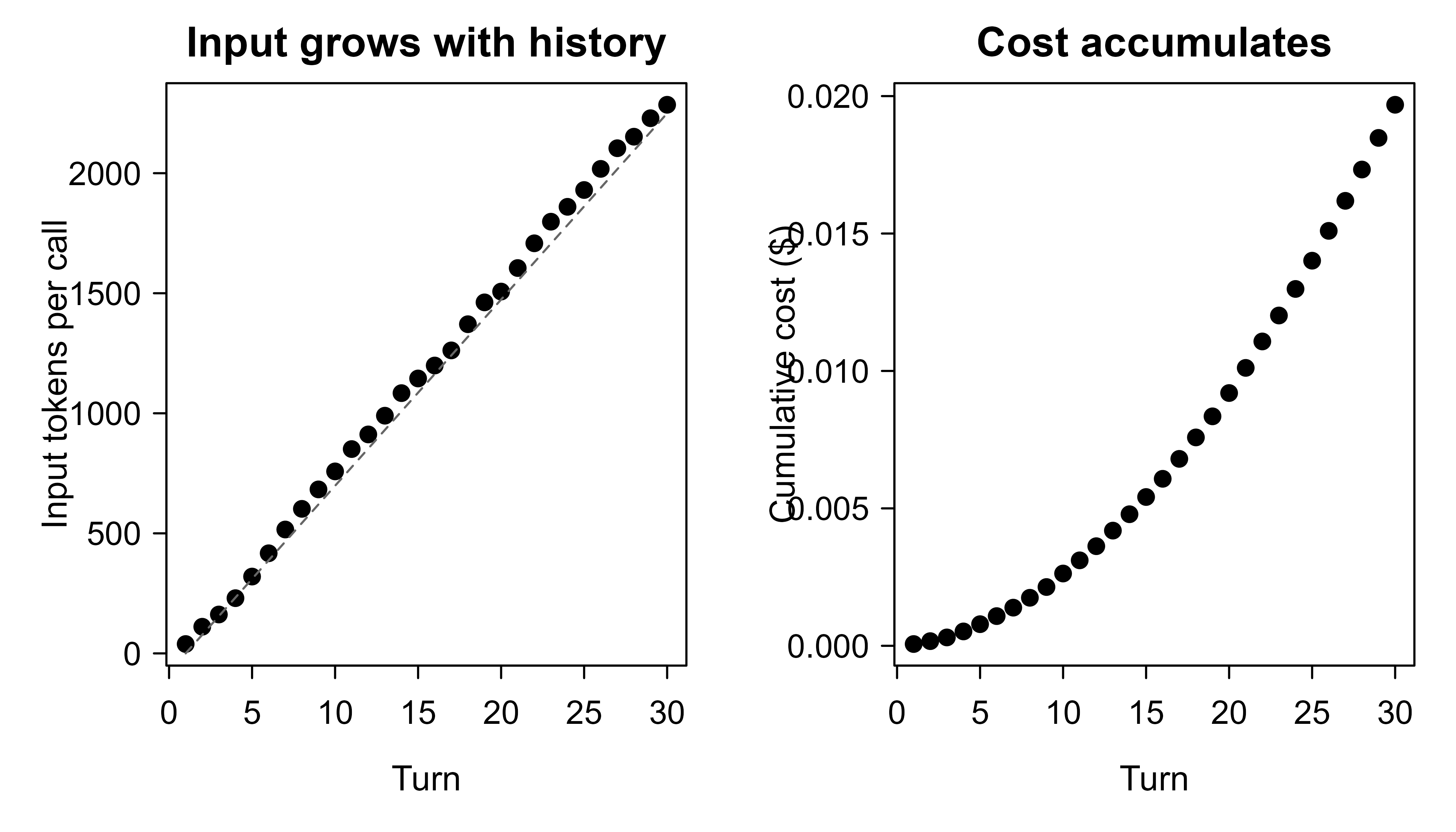
Figure 108.1 plots the two quantities side by side. The dashed line on the left panel is the linear-in-\(k\) approximation \(a(k-1)\) for the per-call input; the cumulative cost on the right is its running sum, which curves upward. The practical lesson: a chat that runs for hundreds of turns can cost far more than the same number of independent one-shot calls, and trimming history is the lever that controls it.
108.5 A Base-R Mock Chat Engine
The cost demo treated tokens as numbers. To see the turn machinery itself, here is a small mock of a chat object. It stores turns, “responds” with canned text keyed on the user message, resends the full history conceptually, and reports token usage exactly as a real client would. No network, no key, fully reproducible. Reading it is the fastest way to understand what ellmer’s chat object does under the surface.
Show code
new_chat <- function(system_prompt = NULL) {
  turns <- list()
  if (!is.null(system_prompt)) {
    turns[[1]] <- list(role = "system", content = system_prompt)
  }
  # Canned "model": deterministic replies so the demo is reproducible.
  respond <- function(user_msg) {
    if (grepl("bias", user_msg, ignore.case = TRUE)) {
      "Bias is error from wrong assumptions; variance is sensitivity to the sample."
    } else if (grepl("knn|nearest", user_msg, ignore.case = TRUE)) {
      "Small k means low bias and high variance; large k means the opposite."
    } else {
      "I am a mock model and only answer questions about bias, variance, or kNN."
    }
  }
  count_tokens <- function(text) ceiling(nchar(text) / 4)

  list(
    chat = function(user_msg) {
      # Append the user turn, then condition the reply on the FULL history.
      turns[[length(turns) + 1]] <<- list(role = "user", content = user_msg)
      reply <- respond(user_msg)
      turns[[length(turns) + 1]] <<- list(role = "assistant", content = reply)
      reply
    },
    get_turns = function() turns,
    get_tokens = function() {
      # Input tokens billed on a call = all prior turns + the new user turn.
      # We reconstruct that per assistant turn to mirror real billing.
      contents <- vapply(turns, function(t) t$content, character(1))
      tok      <- count_tokens(contents)
      roles    <- vapply(turns, function(t) t$role, character(1))
      input_billed <- 0
      running <- 0
      for (i in seq_along(turns)) {
        if (roles[i] == "assistant") input_billed <- input_billed + running
        running <- running + tok[i]
      }
      out_tok <- sum(tok[roles == "assistant"])
      c(input = input_billed, output = out_tok)
    }
  )
}

chat <- new_chat(system_prompt = "You are a terse ML tutor.")
chat$chat("Explain the bias-variance tradeoff.")
#> [1] "Bias is error from wrong assumptions; variance is sensitivity to the sample."
chat$chat("How does it show up in kNN?")
#> [1] "Small k means low bias and high variance; large k means the opposite."

# Inspect the turn list: roles alternate user/assistant after the system turn.
do.call(rbind, lapply(chat$get_turns(),
        function(t) data.frame(role = t$role, content = substr(t$content, 1, 50))))
#>        role                                            content
#> 1    system                          You are a terse ML tutor.
#> 2      user                Explain the bias-variance tradeoff.
#> 3 assistant Bias is error from wrong assumptions; variance is
#> 4      user                        How does it show up in kNN?
#> 5 assistant Small k means low bias and high variance; large k

chat$get_tokens()
#>  input output
#>     58     37
The mock reproduces the two facts that matter most. First, the model conditions on the entire turn list, not just the latest message. Second, input tokens are billed on the accumulated history, so the third turn pays for the first two. Replacing respond() with a real HTTP call and count_tokens() with the provider’s reported usage turns this into a working client, which is essentially what ellmer is.
108.6 Rate Limits, Retries, and Backoff
So far the model has always answered. In production it sometimes will not, and how you handle that is the difference between a robust pipeline and one that falls over under load.
Providers cap how fast you can call them, usually as requests per minute (RPM) and tokens per minute (TPM). Exceed either and the server returns HTTP 429 (“too many requests”). Transient failures (500s, timeouts, brief network errors) also happen. A production client must retry, but retrying immediately and in lockstep makes things worse: many clients that all failed at once will all retry at the same instant and overload the server again.4 The standard fix is exponential backoff with jitter.
Intuition
“Exponential backoff” means wait longer after each failure, doubling the ceiling each time, so a struggling server gets breathing room. “Jitter” means add randomness to the wait, so two clients that failed together do not retry together. The first prevents hammering; the second prevents resynchronizing.
On the \(r\)-th retry, wait a random time
\[ w_r = U\!\left(0,\; \min(B_{\max},\; b \cdot 2^{\,r})\right), \]
where \(b\) is the base delay, \(B_{\max}\) caps the wait, and \(U(0, m)\) is uniform on \([0, m]\). The doubling \(2^r\) spreads load out exponentially as failures persist; the uniform jitter desynchronizes clients so they do not retry in a thundering herd. The expected wait before the \(r\)-th retry is \(\tfrac12 \min(B_{\max}, b\,2^r)\), so the expected total wait before giving up after \(R\) retries is
\[ \mathbb{E}\!\left[\sum_{r=0}^{R-1} w_r\right] = \frac{1}{2}\sum_{r=0}^{R-1}\min(B_{\max},\, b\,2^{r}). \]
ellmer and its HTTP layer (httr2) implement this for you, honoring the provider’s Retry-After header when present.5
Show code
# ellmer delegates HTTP to httr2, which retries on 429/5xx with
# exponential backoff and jitter by default. You can tune it:
library(httr2)

chat <- chat_openai(model = "gpt-4o-mini")

# Set retry policy on the underlying request (advanced usage):
# req_retry(max_tries = 5, backoff = ~ runif(1, 0, min(60, 2^.x)))
# ellmer exposes sensible defaults; override only if you hit limits often.
The backoff logic itself is simple enough to demonstrate in base R.
Show code
backoff_wait <- function(retry, base = 1, cap = 60) {
  runif(1, 0, min(cap, base * 2^retry))
}

# Expected total wait before giving up after R retries.
expected_total_wait <- function(R, base = 1, cap = 60) {
  0.5 * sum(pmin(cap, base * 2^(0:(R - 1))))
}

set.seed(1301)
sapply(0:6, function(r) round(backoff_wait(r), 2))   # one sampled draw per retry
#> [1]  0.56  1.92  1.46  5.03 10.19 25.53 46.20
sapply(1:6, expected_total_wait)                      # expected cumulative wait
#> [1]  0.5  1.5  3.5  7.5 15.5 31.5
The sampled draws are random but bounded by the doubling cap; the expected cumulative wait grows quickly and then flattens once the per-retry cap binds. Choose the cap and the number of retries so the worst-case total wait fits your latency budget.
108.7 Structured Output and Tool Calling
The features so far return prose. The last two features change what comes back so that your program, not just a human, can use it.
Free text is hard to parse. When you want fields, ask for a schema and let the provider constrain the decoding so the reply is valid JSON matching a type you define. ellmer calls these type specifications and returns parsed R objects, not raw strings. This is the right way to do extraction tasks: instead of regexing the model’s prose, you get a list or data frame directly.
Tip
If you ever find yourself writing a regular expression to pull a number or a category out of the model’s sentence, stop and define a schema instead. Schema-constrained output is more reliable and removes a whole class of parsing bugs.
Show code
library(ellmer)

# Define the shape of the answer.
schema <- type_object(
  sentiment = type_string("positive, negative, or neutral"),
  score     = type_number("confidence from 0 to 1"),
  topics    = type_array(items = type_string())
)

chat <- chat_openai(model = "gpt-4o-mini")
chat$chat_structured(
  "Review: the dashboard is fast but the docs are thin.",
  type = schema
)
# Returns a parsed R list: list(sentiment = "...", score = ..., topics = c(...))
Tool calling lets the model request that your code run a function and return the result, which it then folds into its answer. You register R functions; ellmer advertises their signatures to the model, parses the model’s requested call, runs the function locally, and feeds the result back.
Show code
# Register a real R function as a tool the model can call.
get_quantile <- tool(
  function(x_values, p) as.numeric(quantile(x_values, probs = p)),
  description = "Compute the p-th quantile of a numeric vector.",
  arguments = list(
    x_values = type_array(items = type_number()),
    p        = type_number("probability in [0,1]")
  )
)

chat <- chat_openai(model = "gpt-4o-mini")
chat$register_tool(get_quantile)
chat$chat("What is the 90th percentile of 3, 7, 1, 9, 4, 6?")
Use structured output whenever a downstream program consumes the result. Use tools when the model needs facts or computation it cannot do reliably on its own (arithmetic, database lookups, current data).
108.8 Practical Guidance and Pitfalls
The mechanics above are necessary but not sufficient. The following habits separate a demo that works once from a feature you can put in front of real users and real bills. Each one corresponds to a way LLM features tend to fail in practice.
Warning
Treat every model output as untrusted input from the open internet, because that is effectively what it is. Never eval() returned R code, never run returned SQL unsandboxed, and never let user-supplied text silently rewrite your system prompt. The two pitfalls below on validation and prompt injection are the ones most likely to cause real damage.
- Never hard-code keys. Read them from environment variables (
Sys.getenv("OPENAI_API_KEY")) or a secrets manager. Keep them out of source control, logs, and saved.RData. - Pin the model version. Names like “latest” drift over time and break reproducibility. Record the exact model id alongside your results, the same way you would record a package version.
- Budget tokens explicitly. The whole-history resend makes long chats quadratic in cost. Cap the history, summarize old turns, or use independent one-shot calls when you do not actually need memory.
- Set timeouts and retries. Default to exponential backoff with jitter and honor
Retry-After. Decide a maximum wait so a hung call cannot stall a pipeline. - Expect nondeterminism. Even at temperature 0, outputs can vary across calls and across model updates. For evaluation, fix the model id, run multiple samples, and report variability rather than a single number.
- Validate every output. Treat the reply as untrusted input. Parse structured output against a schema and check ranges; never
eval()returned code or run returned SQL without sandboxing. - Measure against a baseline. Before shipping an LLM feature, compare its accuracy and cost to a cheap conventional model on held-out examples. Often a small classifier wins.
- Watch for prompt injection. If user-supplied text reaches the model, it can contain instructions that hijack your system prompt. Keep tools narrow, sandbox their effects, and do not give the model authority it does not need. Systematic evaluation and guardrails for LLM outputs are the subject of Chapter 113.
When the task is well-specified and you have labels, the models from earlier chapters are usually the better engineering choice. Reach for a hosted LLM when the input is unstructured, labels are scarce, and the cost per call is acceptable for your volume.
108.9 Further Reading
- Vaswani, Shazeer, Parmar, Uszkoreit, Jones, Gomez, Kaiser, and Polosukhin (2017), “Attention Is All You Need”, the transformer architecture behind these models.
- Brown et al. (2020), “Language Models are Few-Shot Learners”, on zero- and few-shot prediction with large models.
- Wickham, Cheng, and the Posit team (2024),
ellmerpackage documentation and vignettes, for the chat object, providers, streaming, structured output, and tools. - Wickham (2023),
httr2package documentation, for the HTTP layer, retries, and backoff thatellmerbuilds on. - Ouyang et al. (2022), “Training language models to follow instructions with human feedback”, on why instruction-tuned chat models behave the way they do.
The name is a play on “LLM” read aloud, in the same spirit as the tidyverse habit of phonetic package names. It is maintained by the same Posit team behind
dplyrandhttr2, so it follows the conventions you already know.↩︎The agent pattern is just tool calling, covered later in this chapter, wrapped in a loop: the model proposes a call, your code runs it, the result goes back to the model, and the cycle repeats until the model produces a final answer.↩︎
Common words are often a single token while rare words, code, and non-English text fragment into many. “tokenization” might be one token; an unusual surname or a hex string might be five. The 4-characters rule is a planning heuristic, not an exact count, which is why
ellmerreports the provider’s real numbers after each call.↩︎This synchronized stampede is called the “thundering herd” problem, and it shows up well beyond LLM APIs: any time many clients react to the same signal at the same moment, they can knock over the service they are all waiting on.↩︎
When a 429 response includes a
Retry-Afterheader, the server is telling you exactly how long to wait. A well-behaved client obeys that instead of using its own guess, which is both more polite and usually faster to recover.↩︎