8  Classification and Regression Trees

Imagine you are trying to predict the price of a house, but instead of writing down a formula, you ask a series of yes-or-no questions. Is the house large? If so, is it in a good neighborhood? If so, is it newly built? Each answer sends you down a different path, and at the end of the path you arrive at a guess. That chain of questions is exactly what a decision tree does, and it is probably the closest thing in statistics to the way people actually reason about decisions.

A tree works by carving the predictor space into a set of simple, non-overlapping regions and then making one constant prediction inside each region. The “questions” are splitting rules of the form “is feature \(X_j\) below some threshold?”, and because each rule splits the data in two and then we split again, the rules naturally form a branching structure that looks like an upside-down tree. The same machinery handles both numeric and categorical responses, which is why the method is called CART, short for Classification And Regression Trees.¹

Key idea

A tree partitions the feature space into regions and predicts a single value per region. For regression, that value is the average response of the training points in the region; for classification, it is the most common class in the region.

The first split, at the top of the tree (the “root”), is usually the one that buys you the largest drop in prediction error, measured by the sum of squared residuals (SSR) for regression. Once that split is chosen, the procedure repeats inside each of the two resulting pieces, and so on.

In this chapter you will learn how a tree is grown one split at a time, how to stop it from memorizing the training data by pruning it back, and how to fit and interpret both regression and classification trees in R. Trees on their own are rarely the most accurate predictors, but they are the building block for some of the most powerful methods in this book, including bagging (Chapter 10), random forests (Chapter 13), and boosting (Chapter 11), so understanding them well pays off later.

When to use this

Reach for a single tree when interpretability matters more than raw accuracy, when you want a model a non-specialist can read off a diagram, or when you suspect the relationship between features and response is genuinely nonlinear and full of interactions. If the truth is close to linear, ordinary linear or logistic regression will usually beat a tree.

It helps to be honest up front about where trees struggle, because most of these weaknesses are the reason the later ensemble chapters exist.

• Categorical predictors with many levels are awkward. A categorical variable with \(q\) unordered values has \(2^{q-1} - 1\) possible ways to split its levels into two groups, and with so many candidate splits the tree can easily latch onto a spurious one and overfit.

• Missing predictor values need special handling. For categorical variables you can treat “missing” as its own category, or you can build surrogate splits, backup rules that mimic the chosen split using other variables when the primary variable is unavailable.²

• Non-binary (multiway) splits are tempting but discouraged. Splitting a node into many children at once shatters the data so quickly that little is left for splits further down the tree.

• Linear-combination splits, which split on a weighted combination of variables (in the spirit of principal-component regression), can improve prediction but cost you the easy interpretability that made trees attractive in the first place.

• Trees are unstable. A small change in the training data can flip an early split and produce a completely different tree, which is another way of saying trees have high variance. Bagging (bootstrap aggregating) is the standard fix, and the instability persists even after pruning.

• Trees produce a non-smooth prediction surface, a staircase of flat regions, which can be a poor match for a genuinely smooth regression function. The MARS procedure (multivariate adaptive regression splines, Chapter 9) is a smoother alternative.

• Trees cannot naturally represent additive structure. Because every split conditions on the splits above it, a clean additive effect of several variables is hard to express, whereas MARS can capture it.

• Most importantly, a single tree usually does not predict as accurately as competing regression and classification methods.

Warning

A single fully grown tree almost always overfits. The variance problem is severe enough that in practice you should either prune aggressively or move to an ensemble of trees. Treat the lone tree as a teaching device and an interpretability tool, not as your final predictor.

Set against those drawbacks, trees have real and durable advantages, which is why they remain so widely used.

• They are easy to explain, even to people with no statistics background.
• They mirror the way humans often make decisions, as a sequence of branching questions.
• They are easy to interpret because you can draw the whole model as a diagram.
• They handle qualitative predictors directly, with no need to create dummy variables.

8.1 Regression Trees

We start with the regression case, where the response is numeric, because the logic is cleanest there. Everything about how the tree is grown carries over to classification later; only the splitting criterion changes.

Say we have \(p\) inputs and a response for each of \(n\) observations, \((x_i, y_i), i = 1, \dots, n\) with \(x_i = (x_{i1}, \dots , x_{ip})^T\)

Suppose that we have a partition of the predictor space into \(J\) regions \(R_1, \dots, R_J\) . Then, our prediction in each region is some constant, \(c_j\). Thus, we could write the response function as

\[ f(x) = \sum_{j=1}^J c_j I (x \in R_j) \]

where \(I(x \in R_j)\) is an indicator function (1 when \(x\) is in the j-th region, 0 otherwise). In words, the fitted function is flat inside each region and simply hands back that region’s constant.

Given the partitions, the estimate \(\hat{c}_j\) is the average of of \(y_i\) in \(R_j\)

\[\hat{c}_j = \hat{y}_{R_j} \equiv ave(y_i |x_i \in R_j)\]

This is the natural choice: within a region the prediction that minimizes squared error is the mean of the responses there. To find the partitions, we seek to divide the predictor space into high-dimensional rectangles (boxes) (i.e., we want to find the boxes \(R_1, \dots, R_J\) that minimize the residual sum of squares)

\[ \sum_{j=1}^J \sum_{i \in R_j} (y_i - \hat{y}_{R_j})^2 \]

where \(\hat{y}_{R_j}\) is the mean response for the training observations within the j-th box (e..g, \(\hat{c}_j\) )

Note

Why rectangles? Restricting the regions to axis-aligned boxes is what makes a tree readable. Each split asks about one variable at a time, so every region is described by a simple list of “this variable above this value, that variable below that value” conditions.

Since we can’t consider every possible partition (computationally constraint), we seek binary partitions and specifically, a top down, greedy approach (i.e., at each step the best split is made at that step, once we make a split, we don’t go back and change it) known as recursive binary splitting.

Intuition

“Greedy” means the algorithm grabs the single best split available right now without worrying about whether a slightly worse split today might enable a much better split tomorrow. This is not guaranteed to find the globally optimal tree, but searching all trees is computationally hopeless, and the greedy tree is fast and usually good enough.

8.1.1 Recursive Binary Splitting

Step 1: we select the predictors \(X_j\) and the cutpoints such that splitting the predictor space into the regions \(\{ X|X_j <s\}\) and \(\{ X | X_j \ge s\}\) leads to the maximum reduction in RSS (i.e., for any j and s, we define the regions (half-planes):

\[ R_1 (j,s) = \{ X|X_j <s\} ; R_2(j,s) = \{ X|X_j \ge s\} \]

and seek the value of j and s the minimizes

\[ \sum_{i: x_i \in R_1 (j,s)} (y_i - \hat{y}_{R_1})^2 + \sum_{i: x_i \in R_2 (j,s)} (y_i - \hat{y}_{R_2})^2 \tag{8.1}\]

where \(\hat{y}_{R_1} = \hat{c}_1\) is the mean response in \(R_1(j,s)\)

8.1.1.1 Why the region constant is the mean, and the split objective

Before describing the search over splits, it is worth deriving the two facts that the procedure rests on. Both follow from a single observation about squared error.

Fix any region \(R\) containing the index set \(\{i : x_i \in R\}\) of size \(n_R\), and suppose we must predict a single constant \(c\) for every point in \(R\). The within-region squared-error loss is \(L(c) = \sum_{i \in R} (y_i - c)^2\). Differentiating and setting to zero,

\[ \frac{dL}{dc} = -2 \sum_{i \in R} (y_i - c) = 0 \quad\Longrightarrow\quad \hat c = \frac{1}{n_R} \sum_{i \in R} y_i = \bar y_R , \]

and \(L''(c) = 2 n_R > 0\), so the minimizer is unique and is the region mean. This is exactly the claim \(\hat c_j = \operatorname{ave}(y_i \mid x_i \in R_j)\), now derived rather than asserted. The minimized loss is the within-region sum of squares \(\sum_{i \in R} (y_i - \bar y_R)^2 = n_R \, \widehat{\operatorname{Var}}(y \mid R)\), so minimizing squared error is the same as choosing splits that minimize a weighted sum of within-node response variances.

Because the constant is pinned to the mean, the split search optimizes only over \((j, s)\). Define the parent loss \(Q(R) = \sum_{i \in R} (y_i - \bar y_R)^2\). Splitting \(R\) at \((j,s)\) into children \(R_1(j,s)\) and \(R_2(j,s)\) replaces \(Q(R)\) by \(Q(R_1) + Q(R_2)\), and the impurity reduction is

\[ \Delta(j,s) = Q(R) - \big[\, Q\big(R_1(j,s)\big) + Q\big(R_2(j,s)\big) \,\big] . \]

Since \(Q(R)\) does not depend on the split, minimizing \(Q(R_1)+Q(R_2)\) in Equation 8.1 below is identical to maximizing \(\Delta(j,s)\). The reduction is always nonnegative: \(\bar y_R\) is the single best constant for the pooled data, and allowing two constants can only lower the squared error. A useful algebraic identity is

\[ \Delta(j,s) = \frac{n_{R_1} n_{R_2}}{n_R}\,\big(\bar y_{R_1} - \bar y_{R_2}\big)^2 , \]

so the best split is the one that drives the two child means as far apart as possible, weighted by how evenly it divides the data. This is the regression analogue of a two-sample mean contrast and explains why a feature that cleanly separates high from low responses is favored.

8.1.1.2 Cost of the search

For a continuous predictor \(X_j\), only the \(n_R - 1\) cutpoints lying between consecutive distinct sorted values can change the partition, so the candidate set is finite. A naive evaluation of each candidate from scratch costs \(O(n_R)\), giving \(O(n_R^2)\) per feature. The standard trick is to sort the node’s responses by \(x_{ij}\) once and sweep the cutpoint left to right, maintaining the running counts and sums \(\big(n_{R_1}, \sum_{R_1} y_i\big)\) incrementally. Each child mean, and therefore \(\Delta(j,s)\) via the identity above, then updates in \(O(1)\) per cutpoint, so one feature costs \(O(n_R \log n_R)\) (dominated by the sort) and a node costs \(O(p\, n_R \log n_R)\). Summing over a balanced tree of depth \(O(\log n)\), where each level partitions all \(n\) points, gives an overall growth cost of roughly \(O(p\, n \log^2 n)\). Presorting each feature once at the root reduces the per-node work to a linear scan and is what production implementations do.

Having made that first cut, we treat each resulting piece as a fresh problem and repeat. A few practical points are worth keeping in mind as the tree grows.

• When \(p\) is small, it’s computationally efficient to find values of j and s.

• After the partition is selected, we repeat the process, looking for the best predictor (j) and best cut point (s) to split one of the two new regions to minimize the RSS, which will give us three regions. We continue to split one of these three regions to minimize the RSS

• The stopping criterion is usually when a region contains fewer than some specified number of observations (because we have to the averages of these regressions for our mean response)

• The end regressions of the tree \((R_1, \dots, R_J)\) are known as terminal nodes or leaves of the tree

• The points along the tree where the predictor space is spit are internal nodes

• Regression trees can usually lead to over-fitting on the test set, to reduce this problem, we can prune (i.e., remove leaves) to obtain a subtree using cross-validation.

Tip

Vocabulary you will see everywhere: a leaf (terminal node) is an end region where a prediction is made, an internal node is a point where a split happens, and the connections between them are branches. Pruning means snipping branches off to get a smaller subtree.

8.1.2 Cost complexity pruning

If we grew the tree until every leaf was pure, it would fit the training data beautifully and generalize poorly: classic overfitting. The remedy is to grow a large tree first and then prune it back, keeping only the structure that earns its keep. The technique for doing this is cost complexity pruning, also known as weakest link pruning.

The intuition is a scoring contest among candidate subtrees. We want a tree that fits well but is not bloated with leaves, so we score each candidate by adding a penalty for size.

1. Calculate the total Sum of Squared Residual for each tree

2. Calculate a Tree Score: \(\text{Tree Score} = SSR + \alpha T\) where

   1. SSR = Sum of Squared Residuals for the tree or sub-tree

   2. T = number of leaves (or Terminal nodes) in the tree or sub-tree

   3. \(\alpha\) = tuning parameter (based on cross-validation)

3. Pick tree with lowest tree score

The Tree Complexity Penalty (\(\alpha T\)) compensates for the difference in the number of leaves: a bigger tree only wins if its improvement in fit outweighs the extra penalty it pays for each additional leaf.

More formally, we first grow a very large tree \(T_0\). Instead of considering every possible subtree, we consider a sequence of trees indeed a non-negative tuning parameters, \(\alpha\) (i.e., for each value of \(\alpha\) there is a subtree \(T\) such that \(T \in T_0\) that minimizes

\[ C_\alpha(T) = \sum_{j=1}^{|T|} \sum_{i:x_i \in R_j} (y_i - \hat{y}_{R_j})^2 + \alpha |T| \tag{8.2}\]

where \(|T|\) is the number of terminal nodes

The parameter \(\alpha\) controls a tradoff between the subtree’s complexity and how well it fits the training data (\(\alpha = 0\) implies \(T = T_0\)). As \(\alpha\) gets larger, the penalty for a larger tree is higher, so it penalizes similarly to lasso regression. Moreover, as \(\alpha\) increases, the branches get pruned in a nested a predictable fashion. Hence, it’s possible to get the whole sequence of subtrees as a function of \(\alpha\) (based on cross-validation). After getting \(\alpha\) using cross-validation, we can use that value with the full data set to obtain the fitted subtree

Intuition

The penalty \(\alpha |T|\) plays the same role here that the penalty term plays in lasso regression: it shrinks model complexity. Small \(\alpha\) lets the tree stay large and flexible; large \(\alpha\) forces it down to a stump. The beauty is that as \(\alpha\) slides from 0 upward, the leaves drop off in a single nested sequence, so cross-validation only has to compare a handful of subtrees rather than all of them.

8.1.2.1 The weakest-link algorithm and why the sequence is nested

The claim that the leaves “drop off in a single nested sequence” is not obvious, and it is what makes pruning tractable. A tree with \(|T_0|\) leaves has exponentially many subtrees, so brute-force minimization of Equation 8.2 over all subtrees at every \(\alpha\) would be hopeless. The weakest-link procedure of Breiman et al. proves that the minimizers, taken over all \(\alpha \ge 0\), form a finite nested chain \(T_0 \supset T_1 \supset \cdots \supset \{\text{root}\}\), each \(T_{m+1}\) obtained from \(T_m\) by collapsing a single internal node and the subtree below it.

The argument is local. For any internal node \(t\), let \(T_t\) denote the branch rooted at \(t\) (all of \(t\)’s descendants), let \(R(t) = \sum_{i \in t}(y_i - \bar y_t)^2\) be the squared error if \(t\) were collapsed to a leaf, and let \(R(T_t) = \sum_{\ell \in T_t}\sum_{i \in \ell}(y_i - \bar y_\ell)^2\) be the error of the branch as it stands, with \(|T_t|\) leaves. Collapsing the branch removes \(|T_t| - 1\) leaves. The penalized cost of keeping the branch versus pruning it crosses exactly when

\[ R(t) + \alpha \cdot 1 = R(T_t) + \alpha\,|T_t| \quad\Longrightarrow\quad g(t) = \frac{R(t) - R(T_t)}{|T_t| - 1} . \]

The numerator \(R(t) - R(T_t) \ge 0\) is the extra training error you pay for pruning, and the denominator is the number of leaves you save, so \(g(t)\) is the increase in error per leaf eliminated, the “cost per leaf” of node \(t\). The node with the smallest \(g(t)\) is the weakest link: it is the cheapest branch to remove, and it is the first to be sacrificed as \(\alpha\) rises. The algorithm therefore reads:

1. Start with the full grown tree \(T_0\) (the minimizer at \(\alpha = 0\), up to ties resolved toward the smallest such tree).
2. Compute \(g(t)\) for every internal node, find \(t^\star = \arg\min_t g(t)\), and collapse \(T_{t^\star}\) to a leaf. This yields the next tree in the chain and the breakpoint \(\alpha = g(t^\star)\).
3. Recompute \(g(t)\) on the smaller tree (only ancestors of \(t^\star\) change) and repeat until only the root remains.

This produces a finite increasing sequence of breakpoints \(0 = \alpha_0 < \alpha_1 < \cdots < \alpha_M\) and a matching nested sequence of trees \(T_0 \supset T_1 \supset \cdots \supset T_M\). The key theorem (Breiman et al., 1984) is that for any \(\alpha \in [\alpha_m, \alpha_{m+1})\) the subtree \(T_m\) is the unique smallest minimizer of \(C_\alpha(T)\) over all subtrees of \(T_0\). Cross-validation then needs only to score the \(M+1\) trees in this chain rather than search the full subtree lattice, which is precisely why cv.tree returns error against size over a short list. The same recursion applies verbatim in classification once \(R(\cdot)\) is replaced by the node deviance or misclassification cost.

Note

The cost-per-leaf \(g(t)\) is the discrete analogue of the lasso’s “entry \(\lambda\)” in least-angle regression: both order the model terms by the regularization strength at which they switch off, and both yield a one-dimensional solution path that turns an exponential search into a linear one. The penalty \(\alpha|T|\) is itself an \(\ell_0\)-type complexity penalty (a count of active leaves), so cost-complexity pruning is best-subset selection made feasible by the nesting guarantee, not by relaxation.

8.1.3 Algorithm for regression tree

Putting the pieces together, fitting a regression tree is a three-step recipe: grow, generate a sequence of prunings, then pick the best one by cross-validation.

1. Recursive Binary Splitting for growing a tree with your choice of stopping rule (e.g., observation-based)
2. Use Cost complexity pruning to obtain a sequence of best subtrees as a function of \(\alpha\)
3. Use K-fold cross-validation (see the introduction, Chapter 1) to choose \(\alpha\)

Let us walk through this on the Boston housing data, where the goal is to predict medv, the median home value in a suburb. We grow a tree on a random half of the data so that we can later test it on the half we held out.

library(ISLR2)
library(tree)

set.seed(1)

train <- sample(1:nrow(Boston), nrow(Boston)/2)
tree.boston <- tree(medv ~ ., Boston, subset = train)

# to fit a bigger tree
# tree.boston <-
#     tree(medv ~ .,
#          Boston,
#          subset = train,
#          control = tree.control(nobs = length(train), mindev = 0))

summary(tree.boston) # only 4 vars have been used (rm, lstat, crim, age)
#> 
#> Regression tree:
#> tree(formula = medv ~ ., data = Boston, subset = train)
#> Variables actually used in tree construction:
#> [1] "rm"    "lstat" "crim"  "age"  
#> Number of terminal nodes:  7 
#> Residual mean deviance:  10.38 = 2555 / 246 
#> Distribution of residuals:
#>     Min.  1st Qu.   Median     Mean  3rd Qu.     Max. 
#> -10.1800  -1.7770  -0.1775   0.0000   1.9230  16.5800

Notice that even though the data has many predictors, the tree chose to split on only four of them (rm, lstat, crim, age). Automatic variable selection like this is a side benefit of trees: irrelevant predictors simply never get picked. In the output, deviance = sum of squared errors for the tree, so smaller is better.

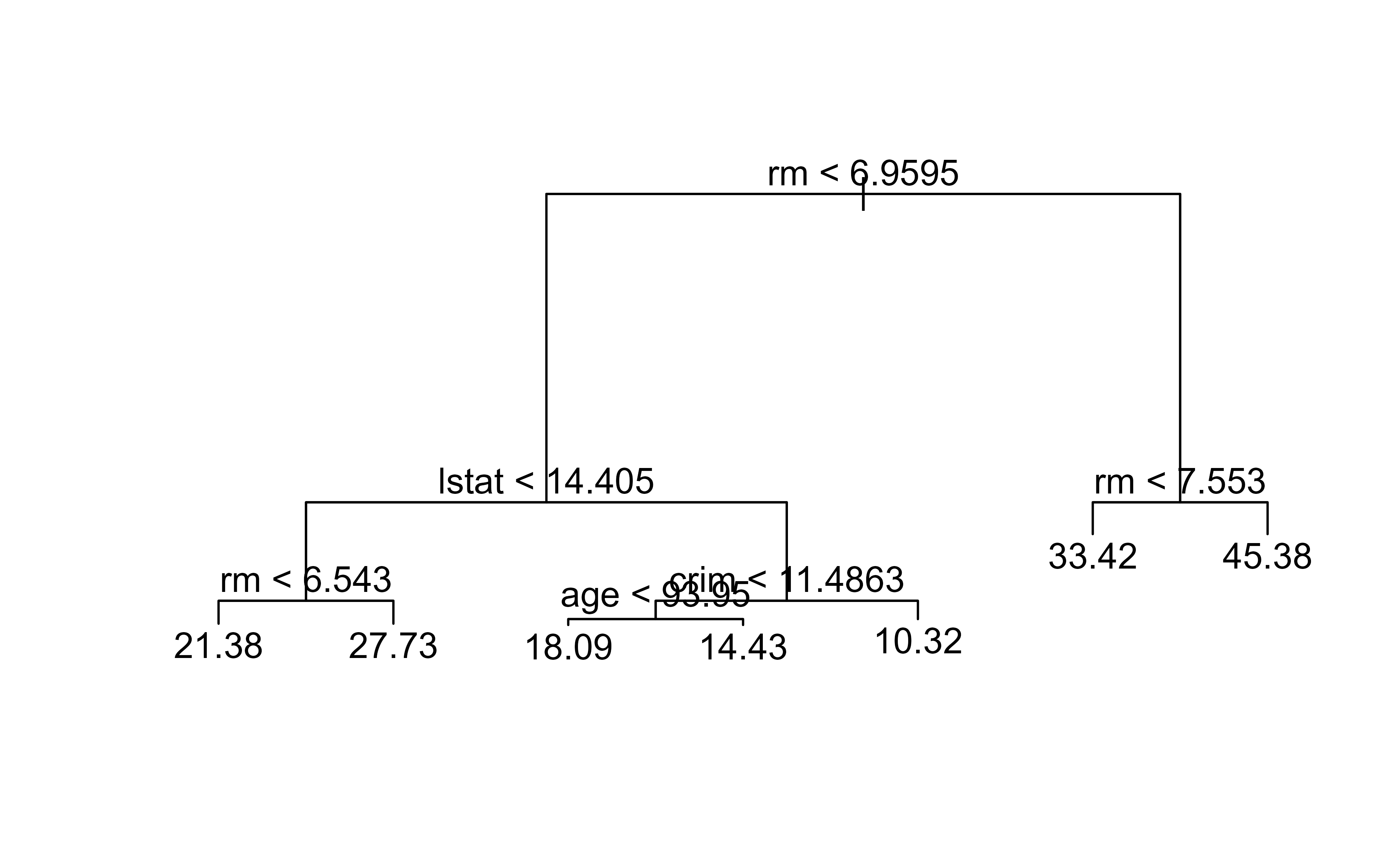
Now we can draw the tree. The text() call labels each split, and reading from the top down gives you the exact sequence of questions the model asks. Figure 8.1 shows the resulting unpruned regression tree fitted to the Boston data.

plot(tree.boston)
text(tree.boston, pretty = 0)

Figure 8.1: Unpruned regression tree fitted to the Boston housing data, predicting median home value from the selected predictors.

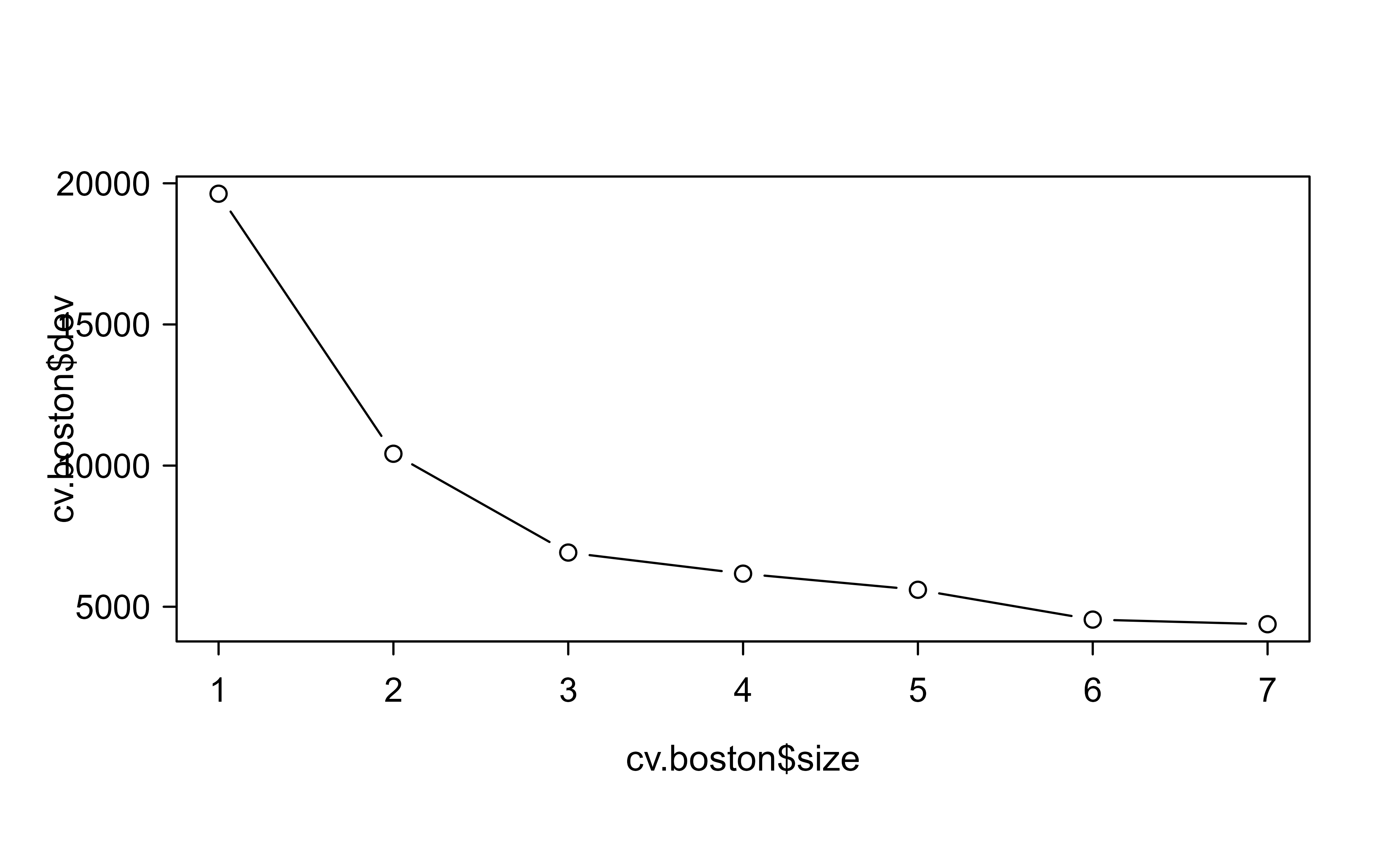
To decide how much to prune, we run cross-validation across tree sizes and look for the size with the lowest cross-validated error. Figure 8.2 plots the cross-validated deviance against tree size.

cv.boston <- cv.tree(tree.boston) # tree complexity selected by cross-validation
plot(cv.boston$size, cv.boston$dev, type = "b")

Figure 8.2: Cross-validated deviance as a function of tree size for the Boston regression tree, used to choose how much to prune.

Tip

Read this plot the way you would read any model-selection curve: error usually drops as the tree grows, then flattens or rises once extra leaves start fitting noise. The smallest tree near the bottom of the curve is the one to prefer, since it is simpler at little or no cost in accuracy.

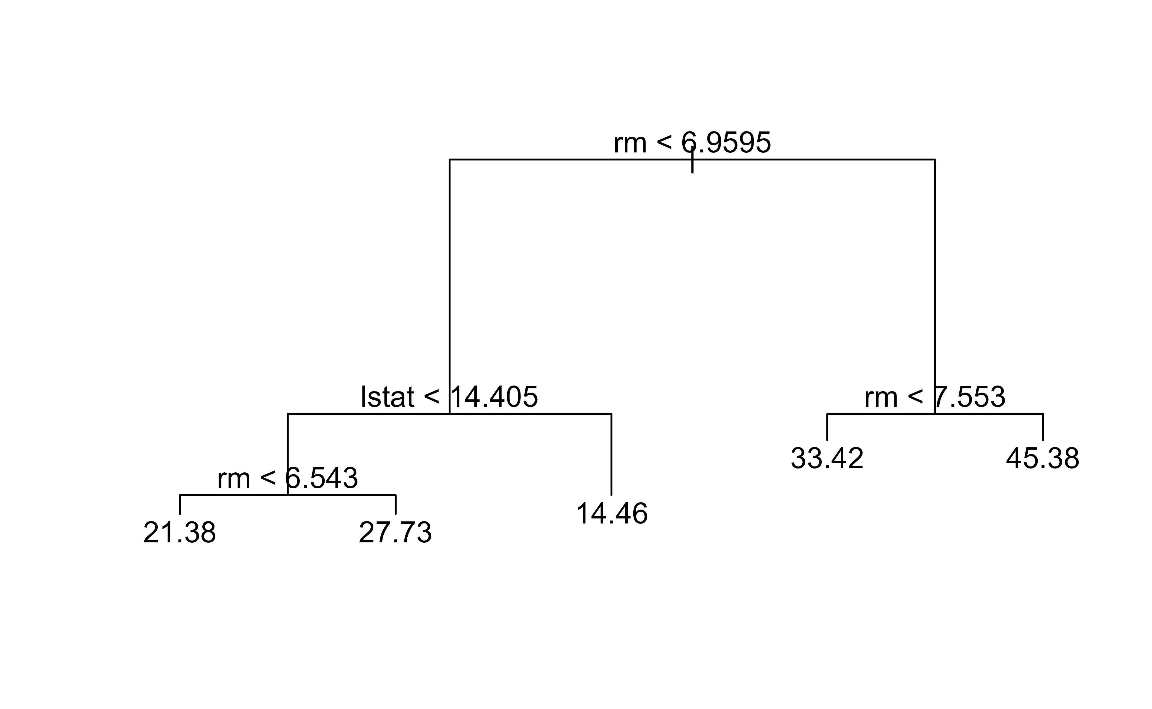
If we want to prune the complex tree back to, say, five leaves, we hand prune.tree() the size we want. Figure 8.3 shows the pruned five-leaf tree.

prune.boston <- prune.tree(tree.boston, best = 5)
plot(prune.boston)
text(prune.boston, pretty = 0)

Figure 8.3: Boston regression tree pruned back to five terminal nodes using prune.tree().

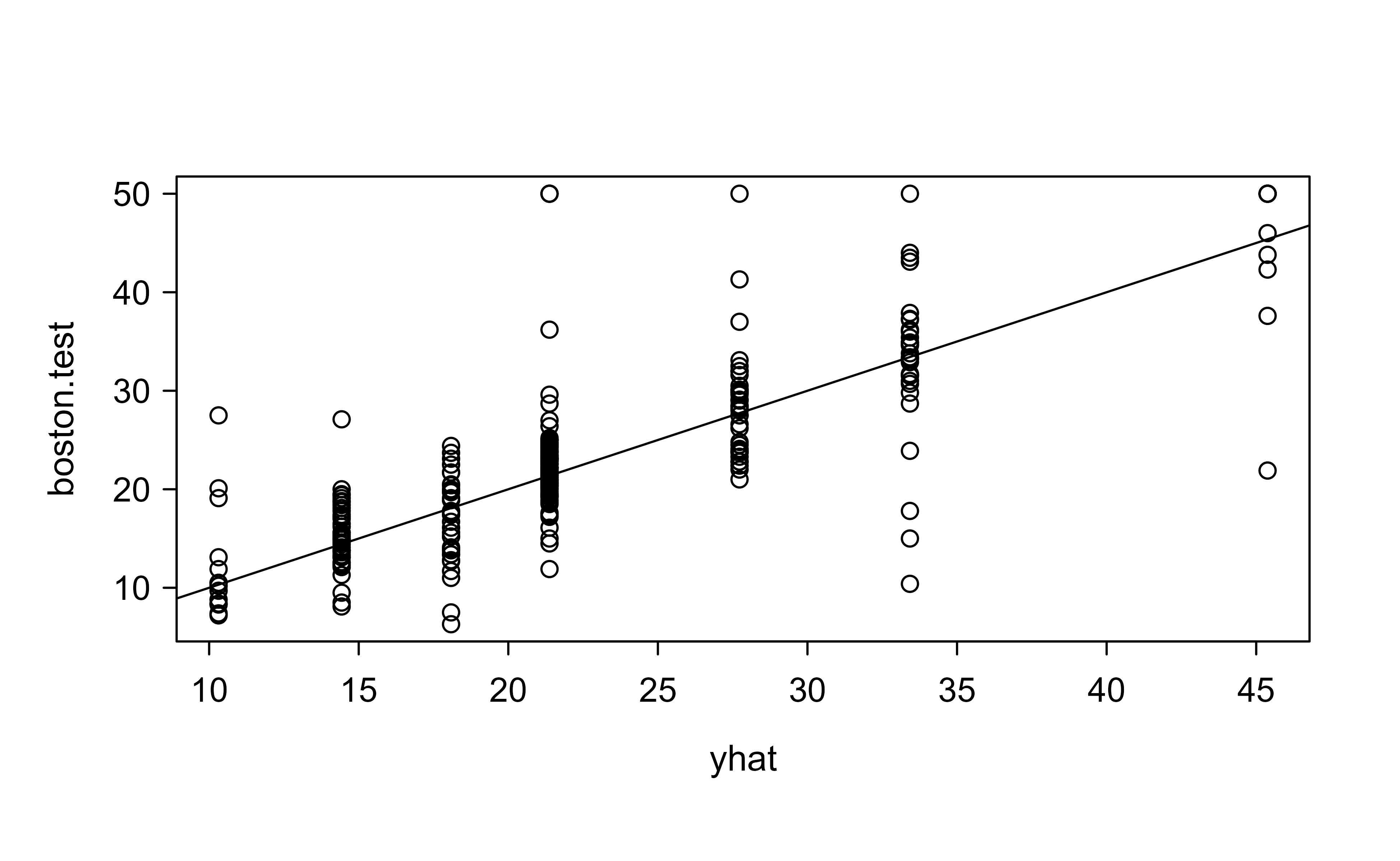
Finally, the real test: how well does the tree predict on the held-out half of the data? We compare predictions against the truth and compute the mean squared error. Figure 8.4 plots the predicted values against the observed test responses.

yhat <- predict(tree.boston, newdata = Boston[-train, ])
boston.test <- Boston[-train, "medv"]
plot(yhat, boston.test)
abline(0, 1)
mean((yhat - boston.test) ^ 2) # Mean squared error
#> [1] 35.28688

Figure 8.4: Predicted versus observed median home values on the held-out Boston test set, with the 45-degree reference line.

The square root of the MSE is 5.9, meaning on average we predict within $5.9k of the true median home value. The points scattering around the 45-degree line (abline(0, 1)) are a quick visual check: the closer they hug that line, the better the predictions.

8.1.4 Statistical properties and failure modes

A tree is a piecewise-constant (histogram-type) regressor, and its behavior is best understood through the bias-variance decomposition. Inside a leaf \(R\) the estimate is the local mean \(\bar y_R\), so its conditional variance is \(\sigma^2 / n_R\): deeper trees have fewer points per leaf and therefore higher variance, while shallow trees average over wide regions and have low variance but high bias because a smooth \(f\) is approximated by a step. Tree depth, controlled in practice through \(\alpha\), the minimum node size, or mindev, is the knob that trades these off, and cross-validation in Equation 8.2 is choosing the point on that curve.

For consistency, suppose \(f\) is continuous and trees are grown so that, as \(n \to \infty\), every leaf diameter shrinks to zero (bias to zero) while the number of points per leaf grows without bound (variance to zero). Under these two conditions the regression tree is universally consistent, \(\mathbb{E}\,[(\hat f_n(x) - f(x))^2] \to 0\). The conditions are exactly the histogram-consistency requirements: a leaf must become both small and well-populated. The catch is the rate. For a \(d\)-dimensional Lipschitz \(f\), an axis-aligned partition estimator attains the minimax rate \(n^{-2/(2+d)}\), the same curse of dimensionality that afflicts kernel and nearest-neighbor methods (Chapter 4). Greedy CART does not always achieve this rate, because its splits are chosen to reduce error on the observed responses rather than to shrink every coordinate uniformly, so a feature that happens to look uninformative early can be starved of splits.

Two structural failure modes follow directly from the axis-aligned, greedy construction.

• Instability (high variance as a function of the data). Because a split is chosen by an \(\arg\max\) over \((j,s)\), two competing splits with nearly equal \(\Delta(j,s)\) can swap under a tiny perturbation of the data, and since every descendant split conditions on the one above it, an early swap cascades into a wholly different tree. This is why a single tree is high-variance even after pruning, and it is the precise weakness that bagging and random forests (Chapter 10, Chapter 13) exploit: averaging many trees fit to resampled data reduces variance without raising bias, because each tree is approximately unbiased but noisy.

• No additive or oblique structure. A true model \(f(x) = g_1(x_1) + g_2(x_2)\) requires the tree to re-split on \(x_2\) inside every \(x_1\) region, spending leaves to reconstruct an effect that an additive model captures in two terms; the data is fragmented exponentially in the number of additive components. Likewise, a linear decision boundary such as \(x_1 > x_2\) can only be approximated by a staircase of axis-aligned cuts, costing many leaves for a boundary MARS (Chapter 9) or a linear model represents exactly. These are not tuning issues; they are intrinsic to the hypothesis class.

Warning

Greedy splitting also creates a selection bias toward features with many candidate cutpoints. A continuous predictor or a categorical one with many levels offers more places to split and so more chances for one split to look good by chance, inflating its apparent importance even when it is noise. Conditional-inference trees (the ctree procedure in the partykit package) address this by separating the choice of splitting variable, via a permutation test, from the choice of cutpoint, which removes the bias at the cost of more computation.

The identity \(\Delta(j,s) = \tfrac{n_{R_1} n_{R_2}}{n_R}(\bar y_{R_1} - \bar y_{R_2})^2\) from Section 8.1.1.1 is easy to confirm numerically, which also serves as a check on the impurity bookkeeping any implementation must get right.

set.seed(1)
y <- rnorm(50); n <- length(y)
Q <- function(v) sum((v - mean(v))^2)
left <- 1:20; right <- 21:50
delta_direct  <- Q(y) - (Q(y[left]) + Q(y[right]))
delta_formula <- (length(left) * length(right) / n) *
    (mean(y[left]) - mean(y[right]))^2
c(direct = delta_direct, formula = delta_formula)
#>    direct   formula 
#> 0.2704538 0.2704538

The two numbers agree, confirming that the impurity reduction equals the weighted squared gap between child means.

8.2 Classification Trees

Everything above was for a numeric response. Often, though, the response is a label rather than a number: spam or not spam, high sales or low sales, disease or healthy. When we have a qualitative response we can use a classification tree.

The main difference from Regression Trees is that we predict the response based on the most commonly occurring class in the region associated with that terminal node.

We may also be interested in the class proportion for each node when interpreting a classification tree, because a leaf that is 95% one class is far more trustworthy than a leaf that is 51% one class, even though both predict the same label.

We grow a classification tree in the same manner as the Regression Trees, with Recursive Binary Splitting. However, instead of using RSS we use other measure related to the classification summary. The reason is simple: squared error is meaningless for a category label, so we need a criterion that rewards splits which make the resulting nodes as “pure” as possible, meaning dominated by a single class.

First we define the proportion of class \(k\) observation in the j-th node as

\[ \hat{p}_{jk} = \frac{1}{n_j} \sum_{x_i \in R_j} I(y_i = k) \]

we classify an observation in node j to class k with the maximum value of \(\hat{p}_{jk}\)

There are three standard measures used to score a split, all of which are smallest when a node is pure.

1. Classification error rate: \(1 - \max_{{k}} (\hat{p}_{jk})\)

   • measures the fraction of the training observations in that region that do not belong to the most common class

2. Gini index: \(\sum_{k=1}^K \hat{p}_{jk}(1 - \hat{p}_{jk})\)

   • measures the total variance across the K classes

3. Cross-Entropy or Deviance: \(-\sum_{k=1}^K \hat{p}_{jk} \log (\hat{p}_{jk})\)

   • related to an information measures and the deviance

The Gini index and Cross-Entory both take small values when all \(\hat{p}_{jk}\) are close to 1 or 0. Hence, we say they measure node purity, which are more sensitive to node probabilities than the classification error rate. Hence, we typically use the last two to grow the tree.

Key idea

Use the Gini index or cross-entropy to grow the tree, because they respond smoothly to changes in class proportions and so produce better splits. Use the classification error rate when your goal is the predictive accuracy of the final pruned tree.

As a rule of thumb: use Gini and cross-entropy to build and prune a tree, and use the classification error rate for pruning if prediction accuracy of the pruned tree is the goal.

8.2.0.1 Why a split criterion must be strictly concave

The preference for Gini and entropy over the misclassification rate has a precise justification: the impurity reduction from a split is guaranteed nonnegative only when the impurity function is concave, and it is guaranteed strictly positive (so the criterion actually rewards informative splits) only when it is strictly concave. The misclassification rate is concave but only piecewise linear, so it can report zero gain for a split that the other two strictly prefer.

Write impurity as a function of the class-proportion vector \(\hat p = (\hat p_1, \dots, \hat p_K)\), and let a split send a fraction \(w_1 = n_{R_1}/n_R\) of the node to child \(R_1\) with proportions \(\hat p^{(1)}\) and \(w_2 = n_{R_2}/n_R\) to \(R_2\) with \(\hat p^{(2)}\). Conservation of counts gives \(\hat p = w_1 \hat p^{(1)} + w_2 \hat p^{(2)}\), so the parent proportion is the weighted average of the children’s. The impurity gain is

\[ \Delta = \phi(\hat p) - \big[\, w_1\,\phi(\hat p^{(1)}) + w_2\,\phi(\hat p^{(2)}) \,\big] . \]

If \(\phi\) is concave, Jensen’s inequality gives \(\phi(\hat p) = \phi\big(w_1 \hat p^{(1)} + w_2 \hat p^{(2)}\big) \ge w_1\phi(\hat p^{(1)}) + w_2\phi(\hat p^{(2)})\), so \(\Delta \ge 0\): any split weakly reduces impurity. The Gini index \(\phi(\hat p) = \sum_k \hat p_k(1-\hat p_k) = 1 - \sum_k \hat p_k^2\) and the entropy \(\phi(\hat p) = -\sum_k \hat p_k \log \hat p_k\) are both strictly concave on the simplex (their Hessians are negative definite on the affine subspace \(\sum_k \hat p_k = 1\)), so the inequality is strict whenever \(\hat p^{(1)} \neq \hat p^{(2)}\). Every split that separates the classes at all strictly improves the score, which gives the search a smooth gradient to follow.

The misclassification impurity \(\phi(\hat p) = 1 - \max_k \hat p_k\) is concave but linear on each region where the same class is the majority. Consider a two-class node with \(\hat p = (0.8, 0.2)\) and a split into children with \((0.9, 0.1)\) and \((0.7, 0.3)\) in equal halves: class 1 is the majority in the parent and in both children, so the misclassification rate is \(0.2\) before and \(\tfrac12(0.1) + \tfrac12(0.3) = 0.2\) after, a gain of zero. Gini, by contrast, drops from \(0.32\) to \(\tfrac12(0.18) + \tfrac12(0.42) = 0.30\), correctly registering that the split purified the node. This is the concrete reason the misclassification rate makes a poor growing criterion: it is blind to splits that shift probability mass without flipping the majority label. It remains the right yardstick for pruning, because there the object of interest is the count of final misclassifications, not the quality of intermediate splits.

For the binary case the three criteria are easy to compare directly. With \(p = \hat p_1\), misclassification is \(\min(p, 1-p)\), Gini is \(2p(1-p)\), and (scaled) entropy is \(-p\log p - (1-p)\log(1-p)\). All three vanish at \(p \in \{0,1\}\) and peak at \(p = \tfrac12\), but only the latter two are strictly concave, and entropy is the most peaked near the pure endpoints, which is why entropy-grown trees tend to keep splitting to push nodes toward purity.

8.2.0.2 Practical choices and diagnostics

A few decisions recur whenever you fit a tree, and the theory above tells you how to make them.

• Stopping versus pruning. Do not rely on a stringent stopping rule (a large minimum node size or a high minimum-gain threshold) to control size. A weak split high in the tree can enable a strong one below it, and a greedy stop never sees it. The robust recipe is to grow deliberately too large, then let cost-complexity pruning and cross-validation in Equation 8.2 choose the size. The minimum node size still matters as a floor: a leaf with one or two points has a wildly variable mean, so values like 5 (regression) or 10 (classification) are common defaults.

• Choosing \(\alpha\). Because \(\alpha\) indexes the finite nested chain of Section 8.1.2.1, cross-validation evaluates only that short list. The one-standard-error rule is standard practice: among trees whose cross-validated error is within one standard error of the minimum, pick the smallest. This buys interpretability and stability at no statistically meaningful cost in accuracy, and it counteracts the optimism of selecting the literal minimum of a noisy curve.

• Categorical predictors. For a \(K\)-class response with an unordered categorical predictor of \(q\) levels, the \(2^{q-1}-1\) possible binary groupings are not all searched in the two-class (or regression) case: ordering the levels by their mean response (regression) or by the proportion of one class (binary classification) and splitting that ordering is provably optimal and reduces the search to \(q-1\) candidates (Breiman et al., 1984; Fisher’s grouping theorem). For multiclass responses no such shortcut exists, which is the practical reason many-level factors are dangerous.

• Cost and scale. Growth costs about \(O(p\,n\log^2 n)\) as derived in Section 8.1.1.2; pruning and cross-validation add a constant factor. Memory is \(O(\text{nodes})\). Trees need no feature scaling, since splits depend only on the order of each feature’s values, and they are invariant to any monotone transformation of an individual predictor, a property linear models lack.

Reading variable importance

A single tree’s split positions are a crude importance signal and inherit the instability of the tree. A more stable summary sums, for each variable, the total impurity reduction \(\Delta\) it produces across all nodes where it is used. Even so, this measure is biased toward high-cardinality and continuous features (the selection bias noted above), so treat single-tree importances as suggestive and prefer the permutation or out-of-bag importances available from the ensemble methods in later chapters.

We illustrate with the Carseats data. The response Sales is continuous, so we first turn it into a binary label High (yes if sales exceed 8, no otherwise) and then predict that label from the other variables.

library(tree)
library(ISLR2)
High <- factor(ifelse(Carseats$Sales <= 8, "No", "Yes")) # transform Sales (conitnuous) to binary variable

Carseats <- data.frame(Carseats, High)

tree.carseats <- tree(High ~ . - Sales, Carseats) # using all variables but Sales

summary(tree.carseats) # training error rate of 9%
#> 
#> Classification tree:
#> tree(formula = High ~ . - Sales, data = Carseats)
#> Variables actually used in tree construction:
#> [1] "ShelveLoc"   "Price"       "Income"      "CompPrice"   "Population" 
#> [6] "Advertising" "Age"         "US"         
#> Number of terminal nodes:  27 
#> Residual mean deviance:  0.4575 = 170.7 / 373 
#> Misclassification error rate: 0.09 = 36 / 400
# tree.carseats

The summary reports a training error rate of about 9%. It also reports a deviance, defined as

\[ -2 \sum_m \sum_k n_{mk} \log \hat{p}_{mk} \]

where \(n_{mk}\) = number of observations in the m-th terminal node in the k-th class. Smaller deviance is preferable (good fit to the training data).

The summary also reports a residual mean deviance, which is just the deviance scaled by the degrees of freedom,

\[ \frac{-2 \sum_m \sum_k n_{mk} \log \hat{p}_{mk}}{n - |T_0|} \]

where \(|T_0|\) = number of terminal nodes. Dividing by \(n - |T_0|\) makes the number comparable across trees of different sizes.

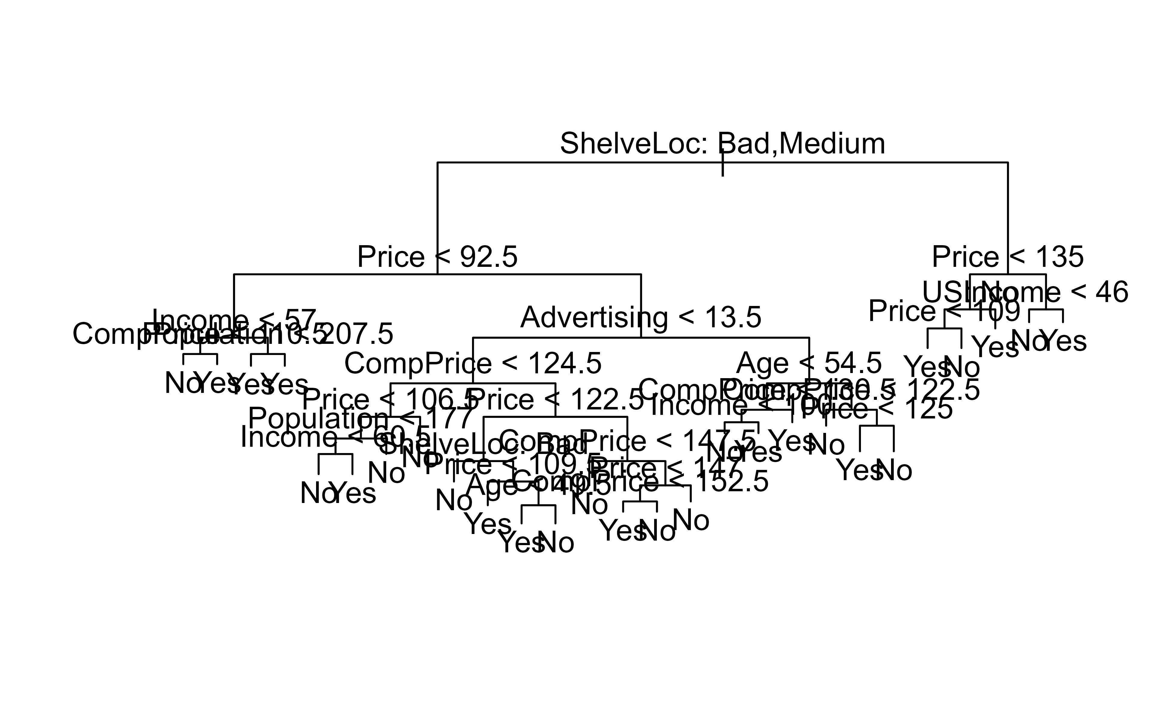
Plotting the tree shows which questions matter most. The variable nearest the root carries the most predictive weight, and here that is the shelving location. Figure 8.5 shows the full classification tree.

plot(tree.carseats)
text(tree.carseats, pretty = 0) # shelving location is the most important indicator

Figure 8.5: Classification tree for the Carseats data predicting whether sales are High, with shelving location as the root split.

A training error rate is optimistic, so the honest evaluation is on data the tree has never seen. We split off 200 observations to train and predict on the rest.

set.seed(1)
train <- sample(1:nrow(Carseats), 200) # index 200 training datapoints

# get the test data
Carseats.test <- Carseats[-train,]

# get actual prediction
High.test <- High[-train]
tree.carseats <- tree(High ~ . - Sales, Carseats, subset = train)

tree.pred <- predict(tree.carseats, Carseats.test, type = "class") # return actual class predidction

table(tree.pred, High.test)
#>          High.test
#> tree.pred No Yes
#>       No  84  37
#>       Yes 35  44

# correct prediction rate
(table(tree.pred, High.test)[1, 1] + table(tree.pred, High.test)[2, 2])/nrow(Carseats.test) # 64% correct predictions
#> [1] 0.64

The cross-tabulation (a confusion matrix) compares predicted labels against true labels; the diagonal entries are correct calls. Dividing the diagonal by the total gives roughly 64% correct on the test set.

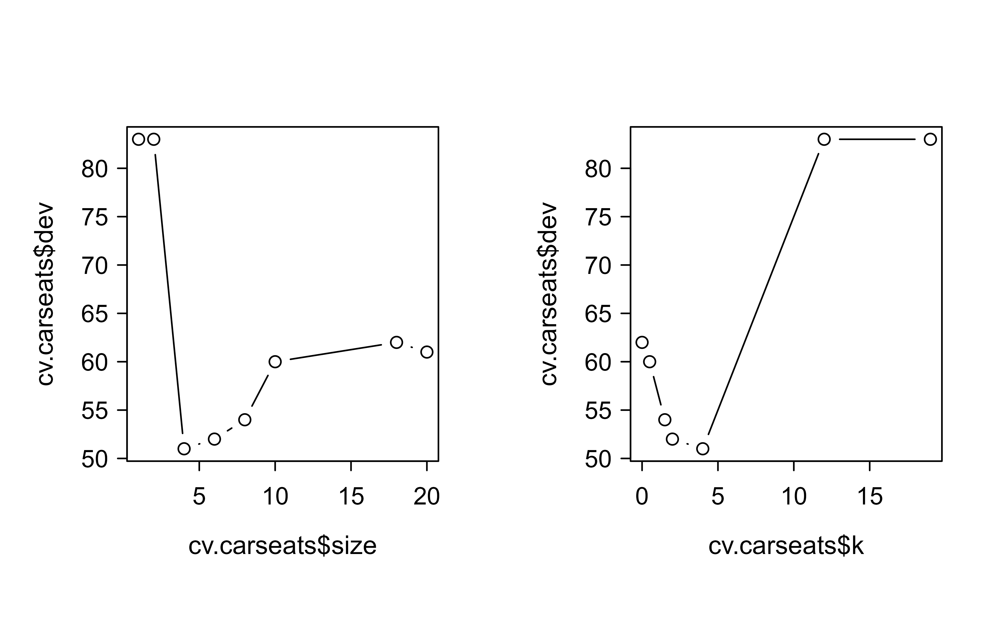
Can we do better by pruning? We cross-validate, this time telling cv.tree() to judge candidate trees by their misclassification rate rather than the default deviance.

set.seed(7)
cv.carseats <- cv.tree(tree.carseats, FUN = prune.misclass) # cross-validation to get the optimal level of tree complexity (depth);
# prune.misclass = classification error rate guides the cross-validation and pruning process
# default = deviance guides the cross-validation and pruning process

cv.carseats
#> $size
#> [1] 20 18 10  8  6  4  2  1
#> 
#> $dev
#> [1] 61 62 60 54 52 51 83 83
#> 
#> $k
#> [1] -Inf  0.0  0.5  1.5  2.0  4.0 12.0 19.0
#> 
#> $method
#> [1] "misclass"
#> 
#> attr(,"class")
#> [1] "prune"         "tree.sequence"

In this output, size = number of terminal nodes of each tree, k = \(\alpha\) = cost-complexity parameter, and dev = number of cross-validation errors.

Note

Despite the name, dev here counts cross-validation errors (misclassifications), not deviance, because we asked for prune.misclass. The tree size with the smallest dev is the one we want.

Plotting error against both tree size and the penalty \(\alpha\) makes the trade-off visible at a glance. Figure 8.6 shows both views side by side.

par(mfrow = c(1, 2))
plot(cv.carseats$size, cv.carseats$dev, type = "b")
plot(cv.carseats$k, cv.carseats$dev, type = "b")

Figure 8.6: Cross-validation errors for the Carseats classification tree plotted against tree size (left) and the cost-complexity parameter (right).

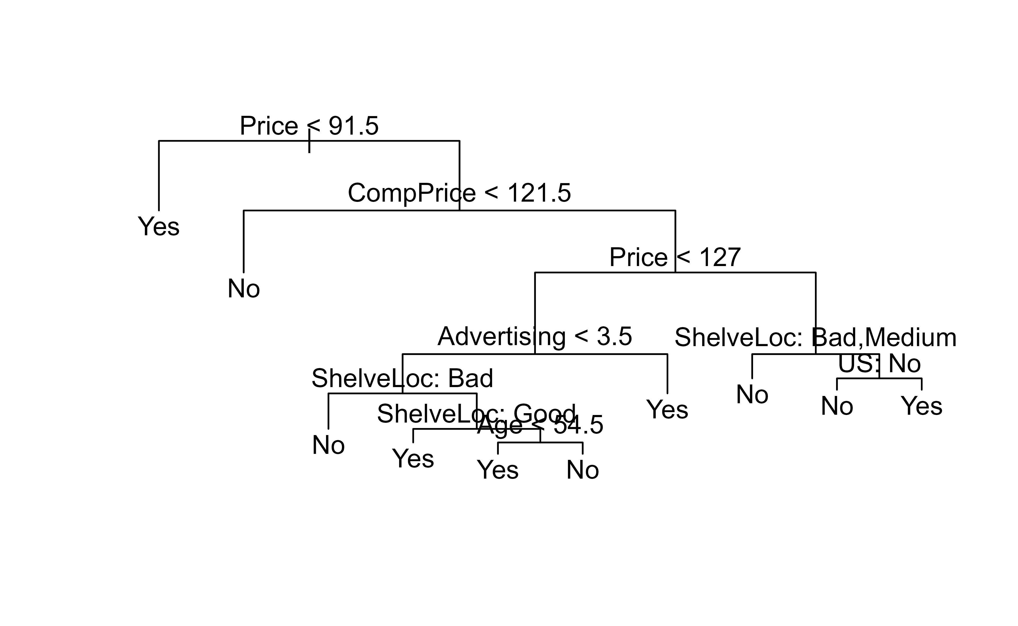
It seems like 9 tree nodes have the lowest number of cv errors (dev in this case). Hence, we will pick this tree and prune to that size. Figure 8.7 shows the resulting nine-leaf pruned tree.

set.seed(7)
prune.carseats <- prune.misclass(tree.carseats, best = 9)
plot(prune.carseats)
text(prune.carseats, pretty = 0)

Figure 8.7: Carseats classification tree pruned to nine terminal nodes, the size with the smallest cross-validation error.

Now we re-evaluate the pruned tree on the same test set to see whether the simpler model actually predicts better.

tree.pred <- predict(prune.carseats, Carseats.test, type = "class")
table(tree.pred, High.test)
#>          High.test
#> tree.pred No Yes
#>       No  89  25
#>       Yes 30  56

(table(tree.pred, High.test)[1, 1] + table(tree.pred, High.test)[2, 2]) /
    nrow(Carseats.test)
#> [1] 0.725

We can see slight improvement of prediction rate from 64 to over 70 percent. This is the pruning payoff in action: a smaller tree generalized better than the larger one, exactly as the overfitting story predicted.

We could keep growing the tree to push training accuracy higher, but only at the price of added complexity and worse generalization. That tension between fit and simplicity is the through-line of this chapter, and it is precisely what the ensemble methods in the following chapters are built to manage.

---

1. The acronym CART comes from the title of the foundational book by Breiman, Friedman, Olshen, and Stone (1984), which introduced the modern version of the algorithm.

2. A surrogate split is a second-best rule that agrees as closely as possible with the primary split on the training data, so it can stand in when an observation is missing the primary variable.