Picture a sheet of rubber laid out as a grid of pins, and a cloud of data points floating in some high-dimensional space above it. Each pin is tied to a position in that high-dimensional space, but the pins are also tied to each other along the sheet, so a pin cannot move far without dragging its neighbors along. Now repeatedly poke the sheet toward wherever the data happen to be dense. Over time the rubber sheet drapes itself over the data cloud, folding and stretching to cover the regions that matter, while the grid structure keeps neighboring pins close together. When you are done, you can read the data by looking at the flat grid instead of the high-dimensional cloud, and points that were close in the original space tend to land on pins that are close on the grid. That draped, neighbor-respecting grid is a self-organizing map.
The self-organizing map (SOM), introduced by Teuvo Kohonen, is two things at once. It is a clustering and vector quantization method, in that it summarizes a dataset by a modest number of prototype vectors, much as K-means does (Chapter 23). It is also a dimension reduction and visualization method, in that those prototypes are arranged on a low-dimensional grid (almost always two-dimensional) whose layout reflects the geometry of the data (Chapter 27). The defining property, the thing that separates a SOM from plain K-means, is that the prototypes are not free to roam independently. They live on the grid and are constrained to be smooth across it, so the map is forced to preserve topology: nearby inputs map to nearby grid cells.
This chapter develops the SOM from the ground up. We start with the competitive learning idea and the online update rule, give a precise mathematical statement, derive the update as a stochastic gradient step on a neighborhood-weighted objective, examine its properties and failure modes, connect it to K-means and to manifold learning, lay out the practical recipe (the U-matrix and component planes), and finish with a small base-R implementation you can run and inspect.
Key idea
A SOM is K-means with a leash. The prototypes minimize a quantization error like K-means, but each update also drags the winner’s grid neighbors along, so the final prototypes vary smoothly across the grid and the map preserves the neighborhood structure of the data.
26.1 Competitive Learning and the SOM Update
The plain-language version of the algorithm is short. We have a grid of units, each carrying a prototype (or codebook, or weight) vector in input space. We show the map one data point at a time. We find the prototype closest to that point, call it the best matching unit (BMU) or winner. We then move the winner toward the data point, and we also move the winner’s grid neighbors toward the data point, by a smaller amount the farther they sit from the winner on the grid. We repeat, slowly shrinking both how far we move (the learning rate) and how wide the neighborhood reaches (the radius). That is competitive learning (units compete to be the winner) with a cooperative twist (the winner shares its prize with its neighbors).
Two distances are in play, and keeping them straight is the whole conceptual content of a SOM. There is distance in the input space, \(\mathbb{R}^p\), used to pick the winner, and there is distance on the grid, the map lattice, used to decide how much each unit cooperates. The map’s magic comes entirely from the interaction between the two.
26.1.1 Setup and notation
Let the data be \(x_1, \dots, x_n \in \mathbb{R}^p\). Fix a grid of \(K\) units, typically a rectangular lattice of size \(q_1 \times q_2\) with \(K = q_1 q_2\). Each unit \(k\) has two coordinates:
a fixed grid position \(r_k \in \mathbb{R}^2\) (for example the integer coordinates of cell \(k\) on the lattice), and
a learnable prototype \(m_k \in \mathbb{R}^p\) in the input space.
The grid positions \(r_k\) never change; they define the map’s geometry. The prototypes \(m_k\) are what learning adjusts. For a presented input \(x\), the best matching unit is the index of the nearest prototype,
Cooperation between units is governed by a neighborhood function \(h_{ck}\), which depends on the grid distance between the winner \(c\) and the unit \(k\). The standard choice is a Gaussian on the lattice,
where \(\sigma > 0\) is the neighborhood radius. Note \(h_{cc} = 1\) (a unit fully cooperates with itself) and \(h_{ck} \to 0\) as a unit gets far from the winner on the grid. A simpler “bubble” neighborhood sets \(h_{ck} = 1\) for units within radius \(\sigma\) of the winner and \(0\) otherwise, which is just a hard-edged version of the same idea.
26.1.2 The online (Kohonen) update
The classic online SOM, presented with input \(x(t)\) at iteration \(t\), updates every prototype toward \(x(t)\) in proportion to its cooperation with the current winner \(c = c(x(t))\):
where \(\alpha(t) \in (0,1)\) is the learning rate. Both \(\alpha(t)\) and the radius \(\sigma(t)\) inside \(h_{ck}(t)\) decay over time, commonly geometrically,
over \(T\) total iterations, from large starting values \((\alpha_0, \sigma_0)\) to small final values \((\alpha_T, \sigma_T)\). Early on, with a wide \(\sigma\), almost every unit moves toward each input and the whole grid unrolls and orients itself globally (the ordering phase). Later, with a narrow \(\sigma\), only the winner and a few immediate neighbors move, so the prototypes settle into a fine quantization of the data (the convergence phase).
Setting \(h_{ck} = \mathbb{1}[k = c]\) (a unit cooperates only with itself) collapses Equation 26.3 to the online version of K-means: only the winning prototype moves toward the data point. So the neighborhood function is precisely the ingredient that turns competitive vector quantization into a topology-preserving map.
Intuition
Think of \(\sigma\) as a zoom level. A large radius means the map cares about getting the big picture right, the global arrangement of regions. A small radius means it cares about local detail, placing each prototype precisely. Annealing \(\sigma\) from large to small is “coarse to fine”: fix the overall shape first, then sharpen.
26.1.3 The batch update
There is also a batch SOM that removes the learning rate and the input ordering entirely, which makes it deterministic given the data and the initialization. Hold \(\sigma\) fixed for a sweep, assign every data point to its BMU, and set each prototype to the neighborhood-weighted mean of all data points,
then shrink \(\sigma\) and repeat. With \(h_{ck} = \mathbb{1}[k=c]\) this is exactly Lloyd’s algorithm for K-means: each prototype becomes the mean of the points assigned to it. The general SOM replaces “mean of my points” with “neighborhood-weighted mean of everyone’s points,” which is what stitches neighboring prototypes together. The batch form is the cleanest way to see the K-means connection, and it is what the kohonen package uses by default.
26.2 Deriving the Update as Descent on a Neighborhood-Weighted Energy
The online rule Equation 26.3 was originally proposed by analogy to biological self-organization rather than derived from an objective, and in its exact form with a fixed neighborhood it is known not to be the gradient of any energy function (the assignment \(c(x)\) and the weights \(h_{ck}\) both depend on the prototypes in a way that does not integrate cleanly). The standard fix, due to Heskes, is to define the BMU using the neighborhood-weighted distortion rather than the raw nearest-prototype distance. Under that definition the SOM does descend a well-defined energy, and the derivation is instructive because it shows exactly where the smoothing comes from.
26.2.1 A neighborhood-weighted distortion
Define the cost of assigning input \(x\) to unit \(k\) not as the squared distance to \(m_k\) alone, but as the neighborhood-weighted squared distance to \(m_k\) and all its grid neighbors,
Choose the winner to minimize this local error, \(c(x) = \arg\min_k e_k(x)\). (When \(\sigma\) is small, \(h_{kj} \approx \mathbb{1}[j=k]\) and this reduces to the ordinary nearest-prototype rule of Equation 26.1.) The total energy summed over the dataset is
Hold the assignments \(c(x_i)\) fixed (they change only at the discrete moments when a point switches winners, contributing nothing to the gradient elsewhere). Differentiating Equation 26.7 with respect to a single prototype \(m_k\),
since only the \(j = k\) term in the inner sum of Equation 26.7 depends on \(m_k\), and \(\tfrac{\partial}{\partial m_k}\lVert x_i - m_k\rVert^2 = -2(x_i - m_k)\). Two routes lead from this gradient to the two SOM variants.
For the online rule, take a stochastic gradient descent step on a single example \(x(t)\) with step size \(\alpha(t)\). The single-sample estimate of Equation 26.8 is \(-h_{c k}\,(x(t) - m_k)\), and the descent step \(m_k \leftarrow m_k - \alpha(t)\,\partial E / \partial m_k\) gives
which is exactly the Kohonen update Equation 26.3. The neighborhood weight \(h_{ck}\), which looked like a heuristic bonus for neighbors, is just the chain-rule factor: input \(x(t)\) pulls on prototype \(m_k\) with strength equal to how much \(k\) cooperates with the winner.
For the batch rule, set the full gradient Equation 26.8 to zero and solve for \(m_k\),
which is the batch update Equation 26.5. So both forms are descent on the same energy: online SGD versus a coordinate-style exact minimization over prototypes with assignments held fixed. This is the same alternating “assign, then update centers” structure as K-means (Chapter 23), and indeed taking \(\sigma \to 0\) in Equation 26.7 recovers the K-means distortion \(\tfrac{1}{2}\sum_i \lVert x_i - m_{c(x_i)}\rVert^2\) exactly.
Why annealing \(\sigma\) is not optional
The energy in Equation 26.7 depends on \(\sigma\) through \(h\). Each value of \(\sigma\) defines a different cost surface. The smoother (large \(\sigma\)) surfaces are gentle and easy to descend but only crudely fit the data; the sharp (small \(\sigma\)) surface is the one we ultimately want but is riddled with poor local minima (twisted, knotted maps). Annealing \(\sigma\) from large to small is a deterministic-annealing schedule: start on an easy surface, track the minimum as it morphs toward the hard one. Holding \(\sigma\) fixed at a small value from the start routinely produces a folded map.
26.3 Properties, Assumptions, and Failure Modes
A few facts make SOMs easier to use well.
Topology preservation is the point, and it is approximate. The map aims to preserve neighborhoods, not distances. Two prototypes that are adjacent on the grid will usually be close in input space, but the converse can fail at the seams where the grid has to fold to cover a curved or branching data manifold. SOMs perform best when the intrinsic dimension of the data is close to the grid dimension (usually two); forcing a high-dimensional, isotropic cloud onto a 2D sheet necessarily distorts something. This is the same tension that all manifold learners face (Chapter 27).
Quantization error versus topographic error. Two complementary diagnostics quantify the two jobs of the map. The quantization error is the mean distance from each point to its BMU, \(\tfrac{1}{n}\sum_i \lVert x_i - m_{c(x_i)}\rVert\), measuring how faithfully the prototypes summarize the data (lower is better, and adding units always lowers it). The topographic error is the fraction of points whose first and second best matching units are not adjacent on the grid, measuring how well topology is preserved (lower is better). The two trade off: a finer grid lowers quantization error but can raise topographic error.
It is not the gradient of a fixed objective in its classic form. As noted, the original online rule with the naive BMU Equation 26.1 does not minimize any single energy; convergence cannot be proven by monotone descent, and in dimension greater than one no general convergence proof exists. In practice the maps do organize reliably under a sensible annealing schedule, and the Heskes form Equation 26.7 restores a clean descent story.
Sensitivity to scaling, initialization, and shape. Because the BMU uses Euclidean distance in input space, features on larger scales dominate; standardize the columns first unless scale is meaningful (the same caution as in K-means clustering). Random prototype initialization works but is slow to order; initializing the prototypes on the plane spanned by the top two principal components (Chapter 27) gives a pre-aligned sheet and much faster, more reproducible convergence. A grid whose aspect ratio matches the data’s leading eigenvalue ratio reduces folding.
Common pathologies. A neighborhood that shrinks too fast yields a folded or knotted map (high topographic error). A learning rate that stays too high never settles. A grid much larger than the data has dead units, prototypes that win for no data point, analogous to empty clusters in K-means. Visual inspection of the U-matrix (below) usually reveals these immediately.
Complexity. Each presentation costs \(O(Kp)\) to find the BMU plus \(O(Kp)\) to update prototypes (the neighborhood weights touch all \(K\) units, though with a hard bubble only the local ones), so one epoch over \(n\) points is \(O(nKp)\). With \(E\) epochs the total is \(O(EnKp)\), linear in everything, which is why SOMs scale comfortably to large datasets. Memory is \(O(Kp)\) for the codebook.
26.4 Reading a Trained Map: U-matrix and Component Planes
A SOM is only as useful as the pictures you draw from it. Two are standard.
The U-matrix (unified distance matrix) visualizes cluster structure on the grid. For each unit, compute the average distance in input space between its prototype and the prototypes of its immediate grid neighbors, then shade the grid by that value. Low values (valleys) mark regions where adjacent prototypes are similar, that is, the interiors of clusters; high values (ridges) mark boundaries where the map has had to stretch across a gap between clusters. Reading a U-matrix is like reading a topographic map: basins are clusters, mountain ranges are the separations between them. This is how a SOM exposes clusters even though, unlike K-means, it never commits to a fixed number of them.
Component planes open up what each input feature contributes. Draw one copy of the grid per feature \(j\), shading unit \(k\) by the \(j\)-th coordinate of its prototype, \(m_{kj}\). Laying the planes side by side shows how each feature varies across the map and, crucially, which features are correlated: two features whose component planes look alike vary together across the data. Component planes turn the SOM into an exploratory tool for understanding feature relationships, not just for clustering.
Beyond these, one typically plots counts (how many data points map to each unit, revealing dense versus empty regions) and, when labels happen to be available, the majority label per unit, which turns the map into a quick visual classifier.
26.5 A Base-R Self-Organizing Map
We now build a small online SOM from scratch on the classic iris measurements, fit a \(7 \times 7\) hexless rectangular grid, and read it through a U-matrix and a component plane. Everything uses base R plus the book’s default plotting setup; nothing beyond standard packages is required. The production package kohonen is shown afterward with eval: false.
Show code
set.seed(1301)## --- Data: scale the four iris measurements (BMU uses Euclidean distance) ---X<-scale(as.matrix(iris[, 1:4]))species<-iris$Speciesn<-nrow(X); p<-ncol(X)## --- Grid: q1 x q2 rectangular lattice; grid positions r_k are integer cells -q1<-7; q2<-7; K<-q1*q2grid<-expand.grid(gx =seq_len(q1), gy =seq_len(q2))# r_k for each unit## Pairwise grid distances ||r_c - r_k|| (used by the neighborhood function)grid_dist<-as.matrix(dist(grid))## --- Initialize prototypes from the data range (small random codebook) ------M<-matrix(runif(K*p, min =rep(apply(X, 2, min), each =K), max =rep(apply(X, 2, max), each =K)), nrow =K, ncol =p)## --- Annealing schedule (geometric decay of learning rate and radius) -------n_iter<-8000a0<-0.5; aT<-0.01# learning rate alpha_0 -> alpha_Ts0<-max(q1, q2)/2; sT<-0.7# radius sigma_0 -> sigma_T## --- Online Kohonen training loop -------------------------------------------for(tinseq_len(n_iter)){frac<-(t-1)/(n_iter-1)alpha<-a0*(aT/a0)^fracsigma<-s0*(sT/s0)^fracx<-X[sample.int(n, 1), ]# present one random inputd2<-colSums((t(M)-x)^2)# ||x - m_k||^2 for all unitsbmu<-which.min(d2)# best matching unit c(x)h<-exp(-(grid_dist[bmu, ]^2)/(2*sigma^2))# neighborhood weights h_ck## update every prototype toward x, scaled by alpha * h_ck (recycles h by row)M<-M+alpha*(h*(matrix(x, K, p, byrow =TRUE)-M))}## --- Diagnostics: BMU of every point, quantization & topographic error ------bmu_of<-function(z){d2<-colSums((t(M)-z)^2); order(d2)[1:2]# top-2 BMUs}bmus<-t(apply(X, 1, bmu_of))qerr<-mean(sqrt(rowSums((X-M[bmus[, 1], ])^2)))terr<-mean(grid_dist[cbind(bmus[, 1], bmus[, 2])]>1.5)# 1st & 2nd not adjacentround(c(quantization_error =qerr, topographic_error =terr), 3)#> quantization_error topographic_error #> 0.402 0.000
The two error numbers report the two jobs of the map: a low quantization error means the prototypes summarize the data well, and a low topographic error means the grid did not have to fold much to do so.
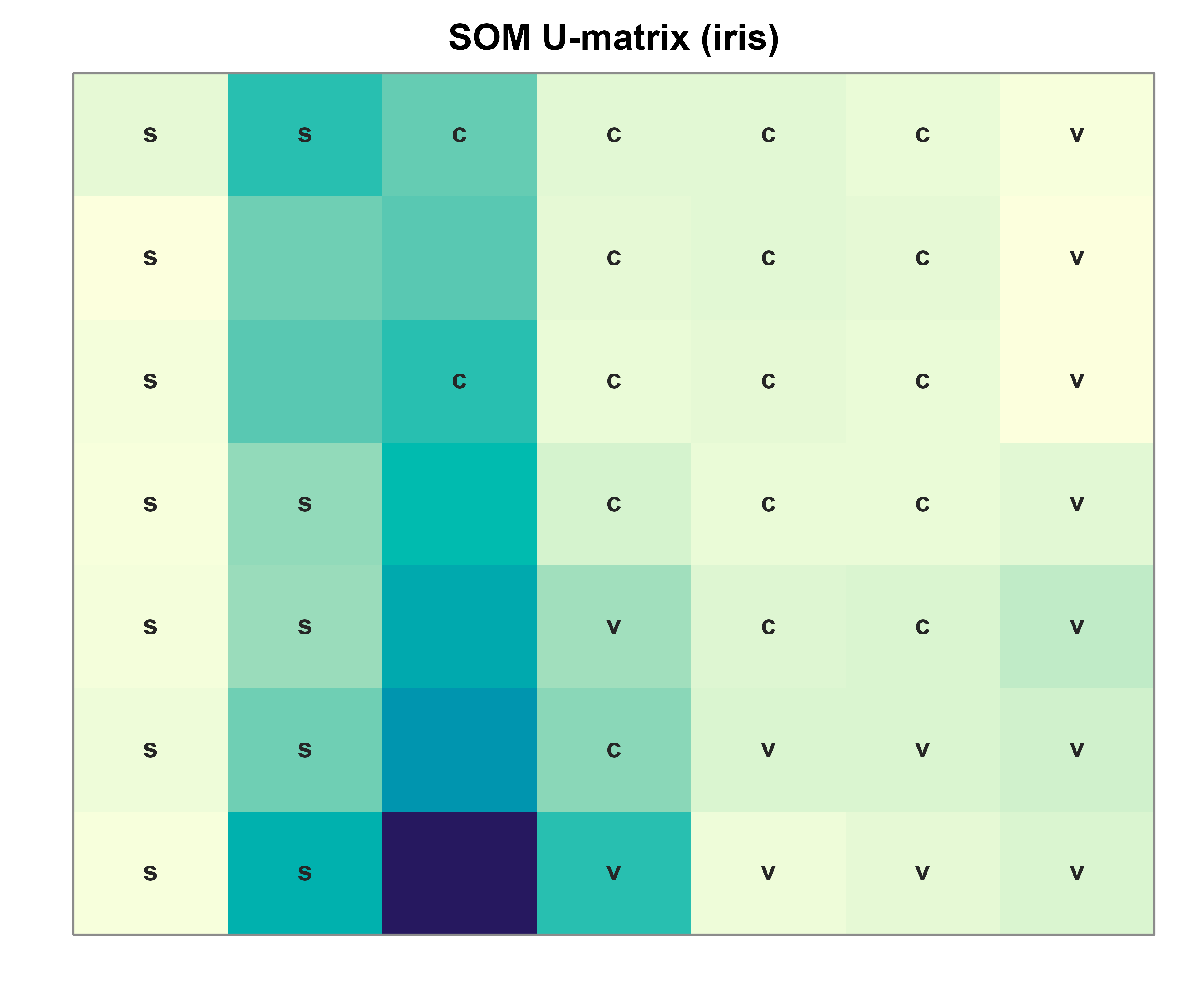
Now the U-matrix. For each unit we average the input-space distance to its grid neighbors, then shade the lattice. Figure 26.1 shows the result, with the dominant species at each unit overlaid so we can confirm the map separated the data.
Show code
## U-matrix: mean distance from each prototype to its immediate grid neighborsumat<-numeric(K)for(kinseq_len(K)){nb<-which(grid_dist[k, ]>0&grid_dist[k, ]<=1.001)# 4-neighborhoodumat[k]<-mean(sqrt(rowSums((M[nb, , drop =FALSE]-matrix(M[k, ], length(nb), p, byrow =TRUE))^2)))}U<-matrix(umat, nrow =q1, ncol =q2)## Dominant species per unit (for overlay)lab_letter<-c(setosa ="s", versicolor ="c", virginica ="v")dom<-rep(NA_character_, K)for(kinseq_len(K)){members<-species[bmus[, 1]==k]if(length(members)>0)dom[k]<-lab_letter[names(which.max(table(members)))]}par(mar =c(2, 2, 2, 1))image(seq_len(q1), seq_len(q2), U, col =hcl.colors(64, "YlGnBu", rev =TRUE), xlab ="", ylab ="", main ="SOM U-matrix (iris)", axes =FALSE)text(grid$gx, grid$gy, labels =ifelse(is.na(dom), "", dom), cex =0.9, col ="grey15", font =2)box(col ="grey55")
Figure 26.1: U-matrix of the trained 7 by 7 SOM on the scaled iris data. Dark valleys are cluster interiors (neighboring prototypes are similar); bright ridges are boundaries. The letter at each unit is the most common species among points whose best matching unit it is (s = setosa, c = versicolor, v = virginica); blank units win no data. The setosa basin is cleanly walled off, while versicolor and virginica share a softer border.
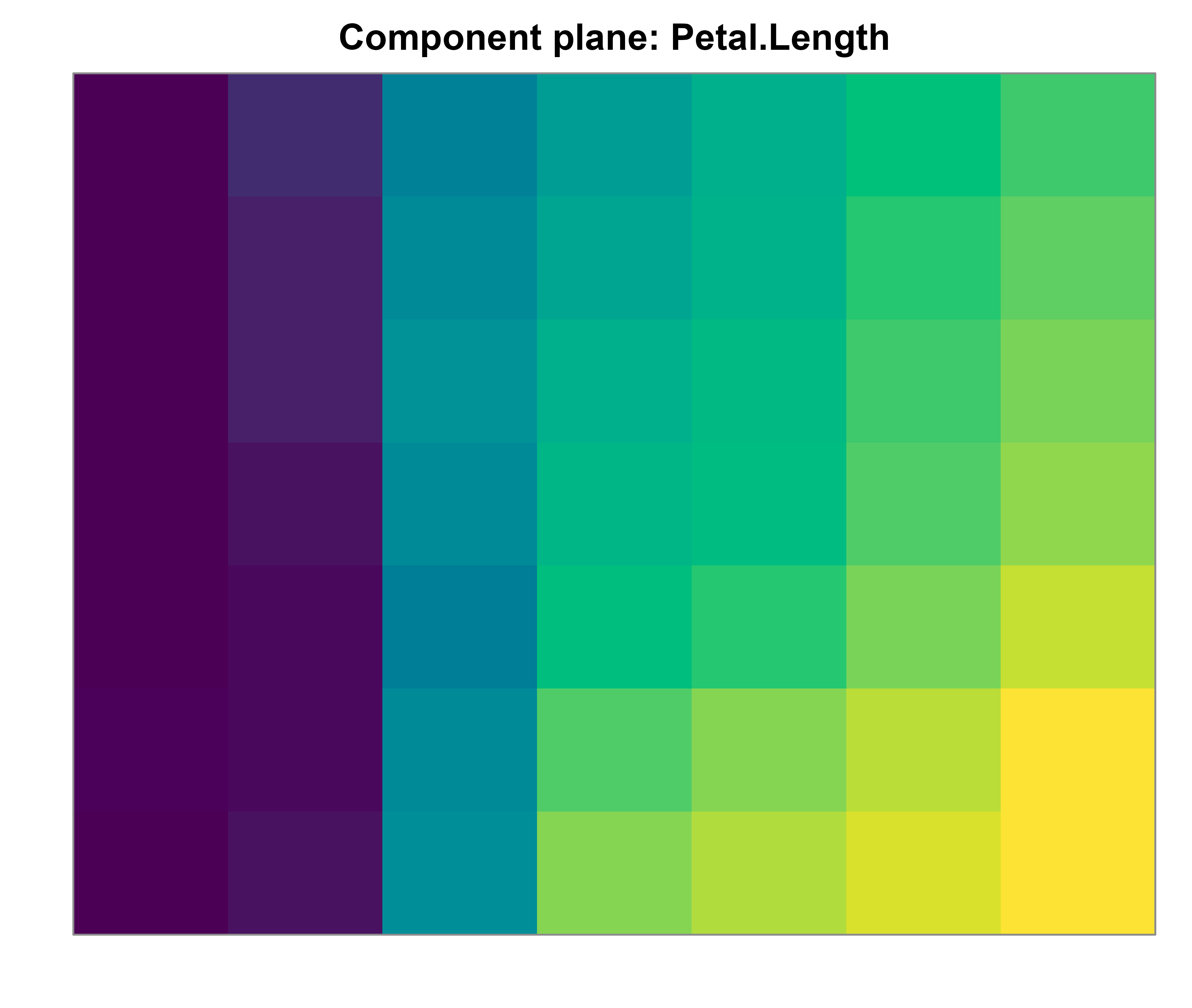
The setosa units cluster in one corner separated from the rest by a bright ridge, exactly the well-known fact that setosa is linearly separable from the other two species while versicolor and virginica overlap. Finally, a component plane in Figure 26.2 shows how one feature, petal length, varies smoothly across the same grid.
Figure 26.2: Component plane for petal length (standardized) across the trained map. Each cell is shaded by its prototype’s petal-length coordinate. The smooth gradient from one corner to the other shows that petal length increases steadily across the map, tracking the setosa-to-virginica ordering visible in the U-matrix.
Comparing the petal-length component plane with the U-matrix shows the feature increasing as we move away from the setosa basin, which is the SOM’s way of telling us that petal length is what most strongly orders these flowers. In a real analysis you would draw all four component planes at once and scan for features whose planes look alike (correlated features) or opposite (anti-correlated), turning the map into an exploratory display of the feature structure.
26.6 Using the kohonen Package
For real work, the kohonen package implements the batch SOM (and the “supersom” extension for multiple data layers) efficiently, with built-in plotting for the U-matrix, counts, and component planes. The snippet below mirrors the analysis above; it is not run here because the package is not installed in this environment.
Show code
library(kohonen)X_iris<-scale(as.matrix(iris[, 1:4]))som_grid<-somgrid(xdim =7, ydim =7, topo ="hexagonal")som_fit<-som(X_iris, grid =som_grid, rlen =500, # number of batch sweeps alpha =c(0.5, 0.01), # online learning rate range (if used) radius =c(4, 0.7))# neighborhood radius scheduleplot(som_fit, type ="dist.neighbours")# U-matrixplot(som_fit, type ="codes")# all component planes at onceplot(som_fit, type ="property", # one component plane property =som_fit$codes[[1]][, "Petal.Length"])plot(som_fit, type ="counts")# data points per unit## Quantization error is reported directly:mean(som_fit$distances)
The topo = "hexagonal" grid is usually preferred over rectangular because each unit then has six equidistant neighbors instead of a mix of four edge and four diagonal neighbors, which makes the neighborhood more isotropic and the U-matrix easier to read.
26.7 Connections to Other Methods
It helps to place the SOM among its relatives.
K-means and vector quantization (Chapter 23). As derived above, a SOM with a zero-radius neighborhood is online K-means, and the batch SOM with zero radius is Lloyd’s algorithm. The neighborhood term is the only difference, and it buys topology preservation at the cost of a small upward bias in quantization error (the prototypes are pulled toward their neighbors rather than sitting at their own cluster means). You can think of a SOM as a smoothness-regularized K-means whose centers live on a graph.
Manifold learning and PCA (Chapter 27). A SOM is a discrete, nonlinear generalization of principal components: PCA fits the best linear subspace, while a SOM fits a flexible 2D sheet that can bend to follow a curved manifold. PCA initialization makes this explicit, since the untrained sheet starts as the top-2 principal plane and then deforms. Unlike t-SNE or UMAP, a SOM produces an explicit, reusable mapping (any new point gets a BMU), and the grid gives a fixed coordinate system rather than a fresh embedding each run.
Density estimation (Chapter 32). The density of data points across the grid (the counts plot) is a coarse, topology-aware estimate of where probability mass concentrates, and the magnification of the map (prototypes are denser where data are denser, though not in exact proportion to the density) connects the SOM to vector-quantization theories of efficient coding.
Neural networks (Chapter 15) and autoencoders (Chapter 41). The SOM is a single-layer competitive (unsupervised) neural network and was historically grouped with them, but it learns by competition and cooperation rather than by backpropagating a reconstruction loss. An autoencoder with a 2D bottleneck plays a similar dimension-reducing role with a smooth, learned, invertible-ish code, whereas the SOM gives a discrete grid and an explicit neighborhood structure that is easier to visualize but coarser.
Takeaways
A self-organizing map is topology-preserving vector quantization: prototypes that minimize a quantization error like K-means, but constrained to vary smoothly across a low-dimensional grid by a decaying neighborhood. The online rule is stochastic gradient descent on a neighborhood-weighted distortion, and the batch rule is its exact-minimization counterpart; both reduce to K-means when the radius goes to zero. Standardize features, anneal the radius from wide to narrow (PCA-initialize for speed), and read the result through the U-matrix (clusters as valleys, boundaries as ridges) and component planes (per-feature structure and correlations). Check both quantization error and topographic error, since a SOM is judged on summarizing the data and on preserving its neighborhoods at once.
Source Code
# Self-Organizing Maps {#sec-self-organizing-maps}```{r}#| include: falsesource("_common.R")```Picture a sheet of rubber laid out as a grid of pins, and a cloud of data points floating in some high-dimensional space above it. Each pin is tied to a position in that high-dimensional space, but the pins are also tied to each other along the sheet, so a pin cannot move far without dragging its neighbors along. Now repeatedly poke the sheet toward wherever the data happen to be dense. Over time the rubber sheet drapes itself over the data cloud, folding and stretching to cover the regions that matter, while the grid structure keeps neighboring pins close together. When you are done, you can read the data by looking at the flat grid instead of the high-dimensional cloud, and points that were close in the original space tend to land on pins that are close on the grid. That draped, neighbor-respecting grid is a self-organizing map.The self-organizing map (SOM), introduced by Teuvo Kohonen, is two things at once. It is a clustering and vector quantization method, in that it summarizes a dataset by a modest number of prototype vectors, much as K-means does (@sec-cluster). It is also a dimension reduction and visualization method, in that those prototypes are arranged on a low-dimensional grid (almost always two-dimensional) whose layout reflects the geometry of the data (@sec-dimension-reduction). The defining property, the thing that separates a SOM from plain K-means, is that the prototypes are not free to roam independently. They live on the grid and are constrained to be smooth across it, so the map is forced to preserve topology: nearby inputs map to nearby grid cells.This chapter develops the SOM from the ground up. We start with the competitive learning idea and the online update rule, give a precise mathematical statement, derive the update as a stochastic gradient step on a neighborhood-weighted objective, examine its properties and failure modes, connect it to K-means and to manifold learning, lay out the practical recipe (the U-matrix and component planes), and finish with a small base-R implementation you can run and inspect.::: {.callout-important title="Key idea"}A SOM is K-means with a leash. The prototypes minimize a quantization error like K-means, but each update also drags the winner's grid neighbors along, so the final prototypes vary smoothly across the grid and the map preserves the neighborhood structure of the data.:::## Competitive Learning and the SOM UpdateThe plain-language version of the algorithm is short. We have a grid of units, each carrying a prototype (or codebook, or weight) vector in input space. We show the map one data point at a time. We find the prototype closest to that point, call it the best matching unit (BMU) or winner. We then move the winner toward the data point, and we also move the winner's grid neighbors toward the data point, by a smaller amount the farther they sit from the winner on the grid. We repeat, slowly shrinking both how far we move (the learning rate) and how wide the neighborhood reaches (the radius). That is competitive learning (units compete to be the winner) with a cooperative twist (the winner shares its prize with its neighbors).Two distances are in play, and keeping them straight is the whole conceptual content of a SOM. There is distance in the input space, $\mathbb{R}^p$, used to pick the winner, and there is distance on the grid, the map lattice, used to decide how much each unit cooperates. The map's magic comes entirely from the interaction between the two.### Setup and notationLet the data be $x_1, \dots, x_n \in \mathbb{R}^p$. Fix a grid of $K$ units, typically a rectangular lattice of size $q_1 \times q_2$ with $K = q_1 q_2$. Each unit $k$ has two coordinates:- a fixed grid position $r_k \in \mathbb{R}^2$ (for example the integer coordinates of cell $k$ on the lattice), and- a learnable prototype $m_k \in \mathbb{R}^p$ in the input space.The grid positions $r_k$ never change; they define the map's geometry. The prototypes $m_k$ are what learning adjusts. For a presented input $x$, the best matching unit is the index of the nearest prototype,$$c(x) = \arg\min_{k \in \{1,\dots,K\}} \; \lVert x - m_k \rVert .$$ {#eq-self-organizing-maps-bmu}Cooperation between units is governed by a neighborhood function $h_{ck}$, which depends on the grid distance between the winner $c$ and the unit $k$. The standard choice is a Gaussian on the lattice,$$h_{ck} = \exp\!\left( -\frac{\lVert r_c - r_k \rVert^2}{2 \sigma^2} \right),$$ {#eq-self-organizing-maps-neighborhood}where $\sigma > 0$ is the neighborhood radius. Note $h_{cc} = 1$ (a unit fully cooperates with itself) and $h_{ck} \to 0$ as a unit gets far from the winner on the grid. A simpler "bubble" neighborhood sets $h_{ck} = 1$ for units within radius $\sigma$ of the winner and $0$ otherwise, which is just a hard-edged version of the same idea.### The online (Kohonen) updateThe classic online SOM, presented with input $x(t)$ at iteration $t$, updates every prototype toward $x(t)$ in proportion to its cooperation with the current winner $c = c(x(t))$:$$m_k(t+1) = m_k(t) + \alpha(t)\, h_{ck}(t)\, \bigl( x(t) - m_k(t) \bigr),\qquad k = 1, \dots, K,$$ {#eq-self-organizing-maps-update}where $\alpha(t) \in (0,1)$ is the learning rate. Both $\alpha(t)$ and the radius $\sigma(t)$ inside $h_{ck}(t)$ decay over time, commonly geometrically,$$\alpha(t) = \alpha_0 \left( \frac{\alpha_T}{\alpha_0} \right)^{t/T},\qquad\sigma(t) = \sigma_0 \left( \frac{\sigma_T}{\sigma_0} \right)^{t/T},$$ {#eq-self-organizing-maps-decay}over $T$ total iterations, from large starting values $(\alpha_0, \sigma_0)$ to small final values $(\alpha_T, \sigma_T)$. Early on, with a wide $\sigma$, almost every unit moves toward each input and the whole grid unrolls and orients itself globally (the ordering phase). Later, with a narrow $\sigma$, only the winner and a few immediate neighbors move, so the prototypes settle into a fine quantization of the data (the convergence phase).Setting $h_{ck} = \mathbb{1}[k = c]$ (a unit cooperates only with itself) collapses @eq-self-organizing-maps-update to the online version of K-means: only the winning prototype moves toward the data point. So the neighborhood function is precisely the ingredient that turns competitive vector quantization into a topology-preserving map.::: {.callout-tip title="Intuition"}Think of $\sigma$ as a zoom level. A large radius means the map cares about getting the big picture right, the global arrangement of regions. A small radius means it cares about local detail, placing each prototype precisely. Annealing $\sigma$ from large to small is "coarse to fine": fix the overall shape first, then sharpen.:::### The batch updateThere is also a batch SOM that removes the learning rate and the input ordering entirely, which makes it deterministic given the data and the initialization. Hold $\sigma$ fixed for a sweep, assign every data point to its BMU, and set each prototype to the neighborhood-weighted mean of all data points,$$m_k \;\leftarrow\; \frac{\displaystyle\sum_{i=1}^n h_{\,c(x_i)\,k}\, x_i}{\displaystyle\sum_{i=1}^n h_{\,c(x_i)\,k}} ,$$ {#eq-self-organizing-maps-batch}then shrink $\sigma$ and repeat. With $h_{ck} = \mathbb{1}[k=c]$ this is exactly Lloyd's algorithm for K-means: each prototype becomes the mean of the points assigned to it. The general SOM replaces "mean of my points" with "neighborhood-weighted mean of everyone's points," which is what stitches neighboring prototypes together. The batch form is the cleanest way to see the K-means connection, and it is what the `kohonen` package uses by default.## Deriving the Update as Descent on a Neighborhood-Weighted EnergyThe online rule @eq-self-organizing-maps-update was originally proposed by analogy to biological self-organization rather than derived from an objective, and in its exact form with a fixed neighborhood it is known not to be the gradient of any energy function (the assignment $c(x)$ and the weights $h_{ck}$ both depend on the prototypes in a way that does not integrate cleanly). The standard fix, due to Heskes, is to define the BMU using the neighborhood-weighted distortion rather than the raw nearest-prototype distance. Under that definition the SOM does descend a well-defined energy, and the derivation is instructive because it shows exactly where the smoothing comes from.### A neighborhood-weighted distortionDefine the cost of assigning input $x$ to unit $k$ not as the squared distance to $m_k$ alone, but as the neighborhood-weighted squared distance to $m_k$ and all its grid neighbors,$$e_k(x) = \frac{1}{2}\sum_{j=1}^{K} h_{kj}\, \lVert x - m_j \rVert^2 .$$ {#eq-self-organizing-maps-localerror}Choose the winner to minimize this local error, $c(x) = \arg\min_k e_k(x)$. (When $\sigma$ is small, $h_{kj} \approx \mathbb{1}[j=k]$ and this reduces to the ordinary nearest-prototype rule of @eq-self-organizing-maps-bmu.) The total energy summed over the dataset is$$E(m_1, \dots, m_K) = \sum_{i=1}^{n} e_{\,c(x_i)}(x_i)= \frac{1}{2}\sum_{i=1}^{n} \sum_{j=1}^{K} h_{\,c(x_i)\,j}\, \lVert x_i - m_j \rVert^2 .$$ {#eq-self-organizing-maps-energy}### Gradient and stochastic stepHold the assignments $c(x_i)$ fixed (they change only at the discrete moments when a point switches winners, contributing nothing to the gradient elsewhere). Differentiating @eq-self-organizing-maps-energy with respect to a single prototype $m_k$,$$\frac{\partial E}{\partial m_k}= \frac{1}{2}\sum_{i=1}^{n} h_{\,c(x_i)\,k}\, \frac{\partial}{\partial m_k}\lVert x_i - m_k \rVert^2= -\sum_{i=1}^{n} h_{\,c(x_i)\,k}\,\bigl( x_i - m_k \bigr),$$ {#eq-self-organizing-maps-grad}since only the $j = k$ term in the inner sum of @eq-self-organizing-maps-energy depends on $m_k$, and $\tfrac{\partial}{\partial m_k}\lVert x_i - m_k\rVert^2 = -2(x_i - m_k)$. Two routes lead from this gradient to the two SOM variants.For the online rule, take a stochastic gradient descent step on a single example $x(t)$ with step size $\alpha(t)$. The single-sample estimate of @eq-self-organizing-maps-grad is $-h_{c k}\,(x(t) - m_k)$, and the descent step $m_k \leftarrow m_k - \alpha(t)\,\partial E / \partial m_k$ gives$$m_k(t+1) = m_k(t) + \alpha(t)\, h_{\,c\,k}\, \bigl( x(t) - m_k(t) \bigr),$$ {#eq-self-organizing-maps-recover}which is exactly the Kohonen update @eq-self-organizing-maps-update. The neighborhood weight $h_{ck}$, which looked like a heuristic bonus for neighbors, is just the chain-rule factor: input $x(t)$ pulls on prototype $m_k$ with strength equal to how much $k$ cooperates with the winner.For the batch rule, set the full gradient @eq-self-organizing-maps-grad to zero and solve for $m_k$,$$\sum_{i=1}^{n} h_{\,c(x_i)\,k}\,\bigl( x_i - m_k \bigr) = 0\;\;\Longrightarrow\;\;m_k = \frac{\sum_{i=1}^{n} h_{\,c(x_i)\,k}\, x_i}{\sum_{i=1}^{n} h_{\,c(x_i)\,k}} ,$$ {#eq-self-organizing-maps-batchsolve}which is the batch update @eq-self-organizing-maps-batch. So both forms are descent on the same energy: online SGD versus a coordinate-style exact minimization over prototypes with assignments held fixed. This is the same alternating "assign, then update centers" structure as K-means (@sec-cluster), and indeed taking $\sigma \to 0$ in @eq-self-organizing-maps-energy recovers the K-means distortion $\tfrac{1}{2}\sum_i \lVert x_i - m_{c(x_i)}\rVert^2$ exactly.::: {.callout-note title="Why annealing $\sigma$ is not optional"}The energy in @eq-self-organizing-maps-energy depends on $\sigma$ through $h$. Each value of $\sigma$ defines a different cost surface. The smoother (large $\sigma$) surfaces are gentle and easy to descend but only crudely fit the data; the sharp (small $\sigma$) surface is the one we ultimately want but is riddled with poor local minima (twisted, knotted maps). Annealing $\sigma$ from large to small is a deterministic-annealing schedule: start on an easy surface, track the minimum as it morphs toward the hard one. Holding $\sigma$ fixed at a small value from the start routinely produces a folded map.:::## Properties, Assumptions, and Failure ModesA few facts make SOMs easier to use well.**Topology preservation is the point, and it is approximate.** The map aims to preserve neighborhoods, not distances. Two prototypes that are adjacent on the grid will usually be close in input space, but the converse can fail at the seams where the grid has to fold to cover a curved or branching data manifold. SOMs perform best when the intrinsic dimension of the data is close to the grid dimension (usually two); forcing a high-dimensional, isotropic cloud onto a 2D sheet necessarily distorts something. This is the same tension that all manifold learners face (@sec-dimension-reduction).**Quantization error versus topographic error.** Two complementary diagnostics quantify the two jobs of the map. The quantization error is the mean distance from each point to its BMU, $\tfrac{1}{n}\sum_i \lVert x_i - m_{c(x_i)}\rVert$, measuring how faithfully the prototypes summarize the data (lower is better, and adding units always lowers it). The topographic error is the fraction of points whose first and second best matching units are not adjacent on the grid, measuring how well topology is preserved (lower is better). The two trade off: a finer grid lowers quantization error but can raise topographic error.**It is not the gradient of a fixed objective in its classic form.** As noted, the original online rule with the naive BMU @eq-self-organizing-maps-bmu does not minimize any single energy; convergence cannot be proven by monotone descent, and in dimension greater than one no general convergence proof exists. In practice the maps do organize reliably under a sensible annealing schedule, and the Heskes form @eq-self-organizing-maps-energy restores a clean descent story.**Sensitivity to scaling, initialization, and shape.** Because the BMU uses Euclidean distance in input space, features on larger scales dominate; standardize the columns first unless scale is meaningful (the same caution as in K-means clustering). Random prototype initialization works but is slow to order; initializing the prototypes on the plane spanned by the top two principal components (@sec-dimension-reduction) gives a pre-aligned sheet and much faster, more reproducible convergence. A grid whose aspect ratio matches the data's leading eigenvalue ratio reduces folding.**Common pathologies.** A neighborhood that shrinks too fast yields a folded or knotted map (high topographic error). A learning rate that stays too high never settles. A grid much larger than the data has dead units, prototypes that win for no data point, analogous to empty clusters in K-means. Visual inspection of the U-matrix (below) usually reveals these immediately.**Complexity.** Each presentation costs $O(Kp)$ to find the BMU plus $O(Kp)$ to update prototypes (the neighborhood weights touch all $K$ units, though with a hard bubble only the local ones), so one epoch over $n$ points is $O(nKp)$. With $E$ epochs the total is $O(EnKp)$, linear in everything, which is why SOMs scale comfortably to large datasets. Memory is $O(Kp)$ for the codebook.## Reading a Trained Map: U-matrix and Component PlanesA SOM is only as useful as the pictures you draw from it. Two are standard.The **U-matrix** (unified distance matrix) visualizes cluster structure on the grid. For each unit, compute the average distance in input space between its prototype and the prototypes of its immediate grid neighbors, then shade the grid by that value. Low values (valleys) mark regions where adjacent prototypes are similar, that is, the interiors of clusters; high values (ridges) mark boundaries where the map has had to stretch across a gap between clusters. Reading a U-matrix is like reading a topographic map: basins are clusters, mountain ranges are the separations between them. This is how a SOM exposes clusters even though, unlike K-means, it never commits to a fixed number of them.**Component planes** open up what each input feature contributes. Draw one copy of the grid per feature $j$, shading unit $k$ by the $j$-th coordinate of its prototype, $m_{kj}$. Laying the planes side by side shows how each feature varies across the map and, crucially, which features are correlated: two features whose component planes look alike vary together across the data. Component planes turn the SOM into an exploratory tool for understanding feature relationships, not just for clustering.Beyond these, one typically plots counts (how many data points map to each unit, revealing dense versus empty regions) and, when labels happen to be available, the majority label per unit, which turns the map into a quick visual classifier.## A Base-R Self-Organizing MapWe now build a small online SOM from scratch on the classic `iris` measurements, fit a $7 \times 7$ hexless rectangular grid, and read it through a U-matrix and a component plane. Everything uses base R plus the book's default plotting setup; nothing beyond standard packages is required. The production package `kohonen` is shown afterward with `eval: false`.```{r}#| label: som-fitset.seed(1301)## --- Data: scale the four iris measurements (BMU uses Euclidean distance) ---X <-scale(as.matrix(iris[, 1:4]))species <- iris$Speciesn <-nrow(X); p <-ncol(X)## --- Grid: q1 x q2 rectangular lattice; grid positions r_k are integer cells -q1 <-7; q2 <-7; K <- q1 * q2grid <-expand.grid(gx =seq_len(q1), gy =seq_len(q2)) # r_k for each unit## Pairwise grid distances ||r_c - r_k|| (used by the neighborhood function)grid_dist <-as.matrix(dist(grid))## --- Initialize prototypes from the data range (small random codebook) ------M <-matrix(runif(K * p,min =rep(apply(X, 2, min), each = K),max =rep(apply(X, 2, max), each = K)),nrow = K, ncol = p)## --- Annealing schedule (geometric decay of learning rate and radius) -------n_iter <-8000a0 <-0.5; aT <-0.01# learning rate alpha_0 -> alpha_Ts0 <-max(q1, q2) /2; sT <-0.7# radius sigma_0 -> sigma_T## --- Online Kohonen training loop -------------------------------------------for (t inseq_len(n_iter)) { frac <- (t -1) / (n_iter -1) alpha <- a0 * (aT / a0)^frac sigma <- s0 * (sT / s0)^frac x <- X[sample.int(n, 1), ] # present one random input d2 <-colSums((t(M) - x)^2) # ||x - m_k||^2 for all units bmu <-which.min(d2) # best matching unit c(x) h <-exp(-(grid_dist[bmu, ]^2) / (2* sigma^2)) # neighborhood weights h_ck## update every prototype toward x, scaled by alpha * h_ck (recycles h by row) M <- M + alpha * (h * (matrix(x, K, p, byrow =TRUE) - M))}## --- Diagnostics: BMU of every point, quantization & topographic error ------bmu_of <-function(z) { d2 <-colSums((t(M) - z)^2); order(d2)[1:2] # top-2 BMUs}bmus <-t(apply(X, 1, bmu_of))qerr <-mean(sqrt(rowSums((X - M[bmus[, 1], ])^2)))terr <-mean(grid_dist[cbind(bmus[, 1], bmus[, 2])] >1.5) # 1st & 2nd not adjacentround(c(quantization_error = qerr, topographic_error = terr), 3)```The two error numbers report the two jobs of the map: a low quantization error means the prototypes summarize the data well, and a low topographic error means the grid did not have to fold much to do so.Now the U-matrix. For each unit we average the input-space distance to its grid neighbors, then shade the lattice. @fig-self-organizing-maps-umatrix shows the result, with the dominant species at each unit overlaid so we can confirm the map separated the data.```{r}#| label: fig-self-organizing-maps-umatrix#| fig-cap: "U-matrix of the trained 7 by 7 SOM on the scaled iris data. Dark valleys are cluster interiors (neighboring prototypes are similar); bright ridges are boundaries. The letter at each unit is the most common species among points whose best matching unit it is (s = setosa, c = versicolor, v = virginica); blank units win no data. The setosa basin is cleanly walled off, while versicolor and virginica share a softer border."#| fig-width: 6.5#| fig-height: 5.5## U-matrix: mean distance from each prototype to its immediate grid neighborsumat <-numeric(K)for (k inseq_len(K)) { nb <-which(grid_dist[k, ] >0& grid_dist[k, ] <=1.001) # 4-neighborhood umat[k] <-mean(sqrt(rowSums((M[nb, , drop =FALSE] -matrix(M[k, ], length(nb), p, byrow =TRUE))^2)))}U <-matrix(umat, nrow = q1, ncol = q2)## Dominant species per unit (for overlay)lab_letter <-c(setosa ="s", versicolor ="c", virginica ="v")dom <-rep(NA_character_, K)for (k inseq_len(K)) { members <- species[bmus[, 1] == k]if (length(members) >0) dom[k] <- lab_letter[names(which.max(table(members)))]}par(mar =c(2, 2, 2, 1))image(seq_len(q1), seq_len(q2), U, col =hcl.colors(64, "YlGnBu", rev =TRUE),xlab ="", ylab ="", main ="SOM U-matrix (iris)", axes =FALSE)text(grid$gx, grid$gy, labels =ifelse(is.na(dom), "", dom),cex =0.9, col ="grey15", font =2)box(col ="grey55")```The setosa units cluster in one corner separated from the rest by a bright ridge, exactly the well-known fact that setosa is linearly separable from the other two species while versicolor and virginica overlap. Finally, a component plane in @fig-self-organizing-maps-component shows how one feature, petal length, varies smoothly across the same grid.```{r}#| label: fig-self-organizing-maps-component#| fig-cap: "Component plane for petal length (standardized) across the trained map. Each cell is shaded by its prototype's petal-length coordinate. The smooth gradient from one corner to the other shows that petal length increases steadily across the map, tracking the setosa-to-virginica ordering visible in the U-matrix."#| fig-width: 6.5#| fig-height: 5.5j <-which(colnames(X) =="Petal.Length")CP <-matrix(M[, j], nrow = q1, ncol = q2)par(mar =c(2, 2, 2, 1))image(seq_len(q1), seq_len(q2), CP, col =hcl.colors(64, "Viridis"),xlab ="", ylab ="", main ="Component plane: Petal.Length", axes =FALSE)box(col ="grey55")```Comparing the petal-length component plane with the U-matrix shows the feature increasing as we move away from the setosa basin, which is the SOM's way of telling us that petal length is what most strongly orders these flowers. In a real analysis you would draw all four component planes at once and scan for features whose planes look alike (correlated features) or opposite (anti-correlated), turning the map into an exploratory display of the feature structure.## Using the `kohonen` PackageFor real work, the `kohonen` package implements the batch SOM (and the "supersom" extension for multiple data layers) efficiently, with built-in plotting for the U-matrix, counts, and component planes. The snippet below mirrors the analysis above; it is not run here because the package is not installed in this environment.```{r}#| eval: falselibrary(kohonen)X_iris <-scale(as.matrix(iris[, 1:4]))som_grid <-somgrid(xdim =7, ydim =7, topo ="hexagonal")som_fit <-som(X_iris, grid = som_grid,rlen =500, # number of batch sweepsalpha =c(0.5, 0.01), # online learning rate range (if used)radius =c(4, 0.7)) # neighborhood radius scheduleplot(som_fit, type ="dist.neighbours") # U-matrixplot(som_fit, type ="codes") # all component planes at onceplot(som_fit, type ="property", # one component planeproperty = som_fit$codes[[1]][, "Petal.Length"])plot(som_fit, type ="counts") # data points per unit## Quantization error is reported directly:mean(som_fit$distances)```The `topo = "hexagonal"` grid is usually preferred over rectangular because each unit then has six equidistant neighbors instead of a mix of four edge and four diagonal neighbors, which makes the neighborhood more isotropic and the U-matrix easier to read.## Connections to Other MethodsIt helps to place the SOM among its relatives.**K-means and vector quantization (@sec-cluster).** As derived above, a SOM with a zero-radius neighborhood is online K-means, and the batch SOM with zero radius is Lloyd's algorithm. The neighborhood term is the only difference, and it buys topology preservation at the cost of a small upward bias in quantization error (the prototypes are pulled toward their neighbors rather than sitting at their own cluster means). You can think of a SOM as a smoothness-regularized K-means whose centers live on a graph.**Manifold learning and PCA (@sec-dimension-reduction).** A SOM is a discrete, nonlinear generalization of principal components: PCA fits the best linear subspace, while a SOM fits a flexible 2D sheet that can bend to follow a curved manifold. PCA initialization makes this explicit, since the untrained sheet starts as the top-2 principal plane and then deforms. Unlike t-SNE or UMAP, a SOM produces an explicit, reusable mapping (any new point gets a BMU), and the grid gives a fixed coordinate system rather than a fresh embedding each run.**Density estimation (@sec-density-estimation).** The density of data points across the grid (the counts plot) is a coarse, topology-aware estimate of where probability mass concentrates, and the magnification of the map (prototypes are denser where data are denser, though not in exact proportion to the density) connects the SOM to vector-quantization theories of efficient coding.**Neural networks (@sec-neural-networks) and autoencoders (@sec-autoencoders).** The SOM is a single-layer competitive (unsupervised) neural network and was historically grouped with them, but it learns by competition and cooperation rather than by backpropagating a reconstruction loss. An autoencoder with a 2D bottleneck plays a similar dimension-reducing role with a smooth, learned, invertible-ish code, whereas the SOM gives a discrete grid and an explicit neighborhood structure that is easier to visualize but coarser.::: {.callout-important title="Takeaways"}A self-organizing map is topology-preserving vector quantization: prototypes that minimize a quantization error like K-means, but constrained to vary smoothly across a low-dimensional grid by a decaying neighborhood. The online rule is stochastic gradient descent on a neighborhood-weighted distortion, and the batch rule is its exact-minimization counterpart; both reduce to K-means when the radius goes to zero. Standardize features, anneal the radius from wide to narrow (PCA-initialize for speed), and read the result through the U-matrix (clusters as valleys, boundaries as ridges) and component planes (per-feature structure and correlations). Check both quantization error and topographic error, since a SOM is judged on summarizing the data and on preserving its neighborhoods at once.:::