Advanced Data Analysis

Nguyen, Mike

121 But-for World

Suppose a competitor opens a store across the street and, over the next year, your sales fall. How much of that decline was actually caused by the new competitor? You cannot simply point at the drop, because sales move for many reasons at once: the season changed, the economy softened, you ran fewer promotions. To answer the question honestly you need to compare what really happened against a careful estimate of what would have happened if the competitor had never arrived. That hypothetical, never-observed world is what economists, marketers, and litigators call the but-for world: the state of affairs that would have prevailed “but for” the event in question.

This chapter introduces the but-for world as a way of thinking, then shows how to turn it into a number. The idea sits at the heart of causal reasoning, and it is the same logic that runs underneath the treatment-effect machinery you met earlier in the book. Here we approach it from the applied side, the way an analyst building a damages model or an impact study would, because that is where the phrase is most often used and where getting it wrong is most costly.¹

Key idea

The effect of an event is the gap between the world we observed and the but-for world we did not. All the difficulty lives in estimating that second, invisible world, because we never get to see it directly.

By the end of the chapter you should be able to state precisely what a but-for world is, recognize the assumptions that make an estimate of it credible, and build a simple counterfactual baseline in R. We will keep the example small on purpose so the logic stays visible, but the same scaffolding scales up to the published studies cited at the end.

121.1 What “but-for” actually means

The but-for world is a counterfactual: a description of how things would have gone under a scenario that did not occur.² In the language of causal inference from the causal machine learning chapter (Chapter 76), it is the potential outcome under no treatment, evaluated for units that were in fact treated.

It helps to fix notation. Let $Y_t^{(1)}$ be the outcome we actually observe at time $t$ after the event, and let $Y_t^{(0)}$ be the outcome that would have occurred at the same time in the but-for world, with no event. The quantity we want, the effect of the event at time $t$, is the difference between them:

\[ \tau_t = Y_t^{(1)} - Y_t^{(0)}. \]

The cumulative effect over a window, the kind of figure that shows up as “lost sales” or “damages,” is just the sum:

\[ \Delta = \sum_{t} \left( Y_t^{(1)} - Y_t^{(0)} \right). \]

The honest problem is that $Y_t^{(0)}$ for the treated period is never observed. Once the competitor enters, every sales figure we record is a $Y_t^{(1)}$. The but-for value $Y_t^{(0)}$ has to be predicted, and that prediction is the entire game.

Intuition

Think of the but-for world as a forecast that ignores the event. You take everything you knew about the outcome before the event, plus anything that kept moving independently of the event, and you project it forward as if the event had never happened. The space between that projection and reality is the estimated impact.

121.2 How the but-for world is estimated

Because $Y_t^{(0)}$ is unobservable, every method for the but-for world is really a strategy for borrowing information from somewhere the event did not reach. There are three common sources, and most serious studies combine them.

The first source is the past. Before the event, the treated unit is its own clean record of life without the event. If sales followed a stable seasonal pattern with a gentle trend, you can fit that pattern on the pre-event data and extrapolate it across the event window. This is the logic of an interrupted time series, and the same forecasting tools covered in the time-series forecasting chapter (Chapter 88) supply the projection; it is the approach we will code below.

The second source is a control group. Somewhere there may be comparable units that the event never touched: stores in cities the competitor did not enter, product lines a layoff did not affect, markets a regulation skipped. If those controls track the treated unit closely before the event, their post-event path is a natural stand-in for the treated unit’s but-for path. Difference-in-differences and synthetic-control methods formalize exactly this borrowing.³

The third source is covariates, other measured variables that drive the outcome but are not themselves affected by the event, such as the overall economy, weather, or category-wide demand. Including them lets the model separate movement caused by the event from movement that would have happened anyway.

When to use this

Reach for a pre-period extrapolation when you have a long, stable history and no good control group. Reach for difference-in-differences or synthetic control when you have credible untreated units. Add covariates whenever common shocks (a recession, a holiday) could otherwise be mistaken for the effect you are measuring.

Whatever the source, the validity of a but-for estimate stands or falls on one assumption: that the relationship you fit before the event would have continued, unchanged, into the event window had the event not occurred. This is the counterfactual analogue of the parallel-trends assumption. It can never be proven, only made plausible, which is why good practice leans so heavily on showing a clean pre-event fit and on testing whether “effects” appear in periods where none should exist.

Warning

A but-for model that fits the pre-event data poorly will produce a damages number anyway, and that number will look just as authoritative as a good one. Always inspect the pre-event fit and stress-test the no-event assumption before you trust the gap.

121.3 A worked example in R

Let us make the idea concrete with a small simulated series. We will create monthly sales that have a trend and a seasonal cycle, introduce an event partway through that depresses sales, and then recover the effect by building a but-for baseline from the pre-event data only. Because we simulate the data, we know the true counterfactual and can check our work, a luxury we never have in practice but a useful one for learning.

We begin by generating the data. The outcome is driven by a linear trend and a twelve-month seasonal pattern; the event arrives at month 37 and knocks a fixed amount off sales each month thereafter.

Show code

set.seed(96)

n_months   <- 60          # five years of monthly data
event_time <- 37          # the event begins here
month_idx  <- 1:n_months

# A smooth trend plus an annual seasonal cycle.
trend    <- 100 + 0.8 * month_idx
seasonal <- 10 * sin(2 * pi * month_idx / 12)
noise    <- rnorm(n_months, mean = 0, sd = 4)

# The true but-for world: what sales would be with no event at all.
y0 <- trend + seasonal + noise

# The true effect: sales drop by 18 units per month after the event.
true_drop <- 18
effect    <- ifelse(month_idx >= event_time, -true_drop, 0)

# The observed world includes the event.
y_obs <- y0 + effect

dat <- data.frame(
  month    = month_idx,
  season   = factor((month_idx - 1) %% 12 + 1),
  observed = y_obs,
  truth0   = y0,
  treated  = month_idx >= event_time
)

head(dat)
#>   month season  observed    truth0 treated
#> 1     1      1 106.07906 106.07906   FALSE
#> 2     2      2 115.89483 115.89483   FALSE
#> 3     3      3 119.79488 119.79488   FALSE
#> 4     4      4 117.29725 117.29725   FALSE
#> 5     5      5 108.43588 108.43588   FALSE
#> 6     6      6  99.21149  99.21149   FALSE

Now we estimate the but-for world using only the pre-event data. We fit a model with a linear trend and seasonal dummies to the first 36 months, then project it across all 60 months. The projection over the post-event window is our estimated $Y_t^{(0)}$, the but-for sales we would have expected with no event.

Show code

pre <- subset(dat, month < event_time)

# Fit trend + seasonality on the clean pre-event period only.
fit <- lm(observed ~ month + season, data = pre)

# Project the fitted relationship across the entire horizon.
dat$but_for <- predict(fit, newdata = dat)

# The estimated effect is observed minus the but-for baseline.
dat$est_effect <- dat$observed - dat$but_for

A but-for model is only as trustworthy as its pre-event fit, so we check that first. If the model tracks the pre-event sales well, we have some reason to believe its post-event projection.

Show code

pre_rmse <- sqrt(mean((dat$observed[dat$month < event_time] -
                       dat$but_for[dat$month < event_time])^2))
round(pre_rmse, 2)
#> [1] 2.91

A small pre-event root mean squared error tells us the baseline reproduces the period it was trained on. Now we can read off the impact. The estimated per-month effect in the post-event window should be close to the true drop of 18 units, and the cumulative gap is our estimate of total lost sales.

Show code

post <- subset(dat, month >= event_time)

avg_effect <- mean(post$est_effect)          # per-month impact
cum_effect <- sum(post$est_effect)           # total "lost sales"

c(estimated_monthly = round(avg_effect, 2),
  true_monthly      = -true_drop,
  estimated_total   = round(cum_effect, 2))
#> estimated_monthly      true_monthly   estimated_total 
#>            -16.46            -18.00           -395.05

The recovered monthly effect lands near the true value of $-18$, and the cumulative figure is our damages-style estimate of everything the event cost over the window. The two numbers differ slightly from the truth because of the random noise in the series, which is exactly the kind of uncertainty a real analysis would have to quantify with confidence intervals, for instance with the distribution-free intervals from the conformal prediction chapter (Chapter 85).

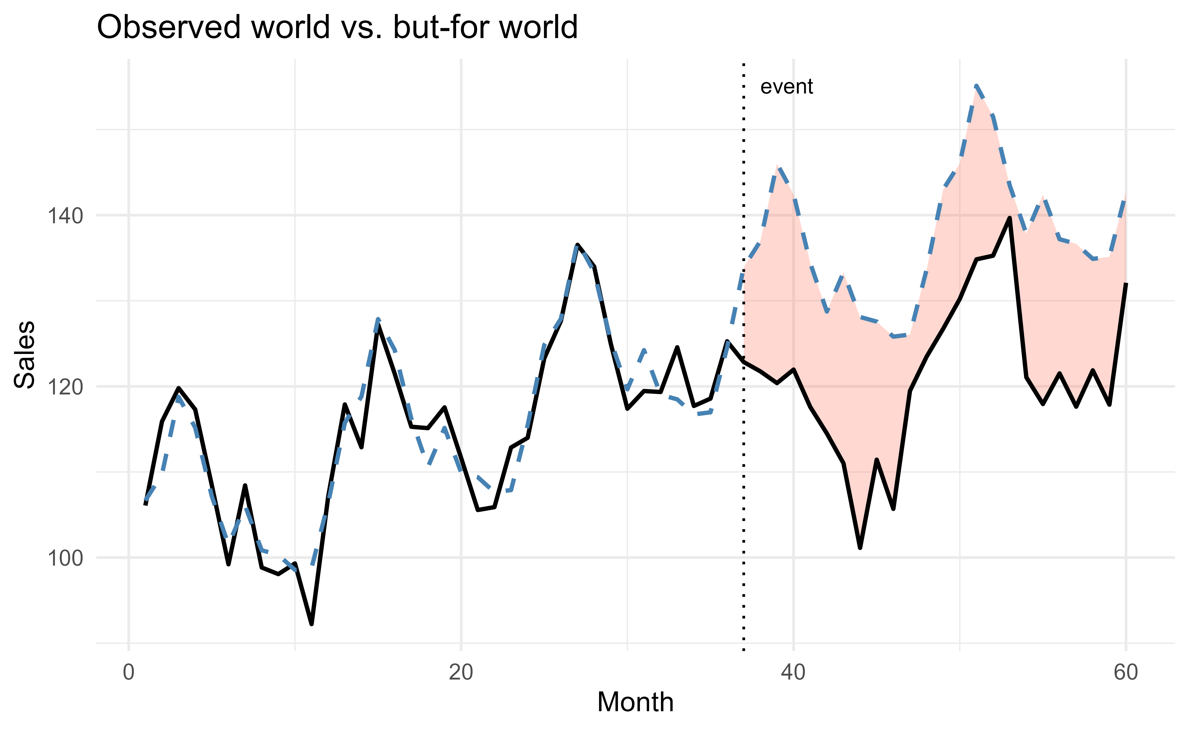
Finally, a picture makes the counterfactual logic obvious. Figure 121.1 plots the observed series, the estimated but-for baseline, and the vertical gap between them after the event.

Show code

library(ggplot2)

ggplot(dat, aes(x = month)) +
  geom_ribbon(
    data = post,
    aes(ymin = observed, ymax = but_for),
    fill = "tomato", alpha = 0.25
  ) +
  geom_line(aes(y = observed), linewidth = 0.8) +
  geom_line(aes(y = but_for), linetype = "dashed", colour = "steelblue",
            linewidth = 0.8) +
  geom_vline(xintercept = event_time, linetype = "dotted") +
  annotate("text", x = event_time + 1, y = max(dat$but_for),
           label = "event", hjust = 0, size = 3) +
  labs(
    x = "Month",
    y = "Sales",
    title = "Observed world vs. but-for world"
  ) +
  theme_minimal()

Figure 121.1: Observed sales (solid) against the estimated but-for baseline (dashed). The shaded gap after the event is the estimated impact, the difference between the world we saw and the world we did not.

The dashed line is the but-for world we constructed; the solid line is what actually happened; the shaded band is the effect. Everything we claimed about the event’s impact is contained in that band, which is why so much care goes into justifying the dashed line.

Tip

Before reporting any number from a plot like this, run a placebo check: pretend the event happened at some earlier date in the pre-event period, refit, and confirm that the estimated “effect” is near zero. A model that finds large effects where none exist is telling you its baseline cannot be trusted.

121.4 From toy model to real studies

The simulated example used the simplest possible counterfactual, a trend-plus-seasonality extrapolation from the unit’s own past. Published work layers on the richer sources of information described above. Mahajan, Sharma, and Buzzell (1993) study the impact of competitive entry on an incumbent’s sales, separating the part of any change that reflects genuine market expansion from the part that reflects sales taken from the incumbent; the but-for world there is the incumbent’s sales path absent the entrant. Landsman and Stremersch (2020) examine what happens to a brand after a collective layoff and a plant closure, asking whether the commercial damage extends to the brand itself; their but-for world is the brand’s commercial trajectory had the plant stayed open. In both cases the analytic task is the one we practiced: estimate the unobserved no-event outcome, then read the effect off the gap.

Note

The methods differ across these studies, but the question does not. Whenever you see a claim about “the effect of X on Y,” look for the but-for world hiding behind it. If the authors cannot tell you clearly what world they are comparing against, treat the effect estimate with suspicion.

121.5 Takeaways

The but-for world reframes “what was the effect of this event?” as “what would have happened without it?”, and that reframing is what makes causal claims tractable. The effect is always a difference between an observed outcome and an estimated counterfactual, $\tau_t = Y_t^{(1)} - Y_t^{(0)}$, with the counterfactual half supplied by a model rather than by observation. Estimating it well means borrowing information from a place the event did not reach, the unit’s own past, a comparable control group, or covariates that moved on their own, and then defending the assumption that the pre-event relationship would have held. The R example showed the whole loop in miniature: fit a baseline on the clean period, project it forward, and measure the gap, while never forgetting that the credibility of the answer rests entirely on the credibility of the baseline.

The term comes from the legal standard for causation. To recover damages, a plaintiff typically must show what their position would have been “but for” the defendant’s conduct, and then claim the difference. The same counterfactual reasoning is used far outside the courtroom whenever we want to isolate the effect of one event from everything else going on.↩︎
A counterfactual is a conditional statement whose premise is contrary to fact, such as “if the competitor had not entered, sales would have been X.” Counterfactuals cannot be observed, only inferred, which is why every but-for analysis rests on a model of some kind.↩︎
A synthetic control builds a weighted average of untreated units that mimics the treated unit’s pre-event behavior, then uses that weighted average as the but-for series afterward. It is the workhorse of modern impact evaluation precisely because it makes the borrowed counterfactual explicit and checkable.↩︎

# But-for World {#sec-but-for-world} ```{r} #| include: false source("_common.R") ``` Suppose a competitor opens a store across the street and, over the next year, your sales fall. How much of that decline was actually caused by the new competitor? You cannot simply point at the drop, because sales move for many reasons at once: the season changed, the economy softened, you ran fewer promotions. To answer the question honestly you need to compare what really happened against a careful estimate of what *would* have happened if the competitor had never arrived. That hypothetical, never-observed world is what economists, marketers, and litigators call the but-for world: the state of affairs that would have prevailed "but for" the event in question. This chapter introduces the but-for world as a way of thinking, then shows how to turn it into a number. The idea sits at the heart of causal reasoning, and it is the same logic that runs underneath the treatment-effect machinery you met earlier in the book. Here we approach it from the applied side, the way an analyst building a damages model or an impact study would, because that is where the phrase is most often used and where getting it wrong is most costly.^[The term comes from the legal standard for causation. To recover damages, a plaintiff typically must show what their position would have been "but for" the defendant's conduct, and then claim the difference. The same counterfactual reasoning is used far outside the courtroom whenever we want to isolate the effect of one event from everything else going on.] ::: {.callout-important title="Key idea"} The effect of an event is the gap between the world we observed and the but-for world we did not. All the difficulty lives in estimating that second, invisible world, because we never get to see it directly. ::: By the end of the chapter you should be able to state precisely what a but-for world is, recognize the assumptions that make an estimate of it credible, and build a simple counterfactual baseline in R. We will keep the example small on purpose so the logic stays visible, but the same scaffolding scales up to the published studies cited at the end. ## What "but-for" actually means The but-for world is a counterfactual: a description of how things would have gone under a scenario that did not occur.^[A counterfactual is a conditional statement whose premise is contrary to fact, such as "if the competitor had not entered, sales would have been X." Counterfactuals cannot be observed, only inferred, which is why every but-for analysis rests on a model of some kind.] In the language of causal inference from the causal machine learning chapter (@sec-causal-machine-learning), it is the potential outcome under no treatment, evaluated for units that were in fact treated. It helps to fix notation. Let $Y_t^{(1)}$ be the outcome we actually observe at time $t$ after the event, and let $Y_t^{(0)}$ be the outcome that would have occurred at the same time in the but-for world, with no event. The quantity we want, the effect of the event at time $t$, is the difference between them: $$ \tau_t = Y_t^{(1)} - Y_t^{(0)}. $$ The cumulative effect over a window, the kind of figure that shows up as "lost sales" or "damages," is just the sum: $$ \Delta = \sum_{t} \left( Y_t^{(1)} - Y_t^{(0)} \right). $$ The honest problem is that $Y_t^{(0)}$ for the treated period is never observed. Once the competitor enters, every sales figure we record is a $Y_t^{(1)}$. The but-for value $Y_t^{(0)}$ has to be *predicted*, and that prediction is the entire game. ::: {.callout-tip title="Intuition"} Think of the but-for world as a forecast that ignores the event. You take everything you knew about the outcome before the event, plus anything that kept moving independently of the event, and you project it forward as if the event had never happened. The space between that projection and reality is the estimated impact. ::: ## How the but-for world is estimated Because $Y_t^{(0)}$ is unobservable, every method for the but-for world is really a strategy for borrowing information from somewhere the event did *not* reach. There are three common sources, and most serious studies combine them. The first source is the past. Before the event, the treated unit is its own clean record of life without the event. If sales followed a stable seasonal pattern with a gentle trend, you can fit that pattern on the pre-event data and extrapolate it across the event window. This is the logic of an interrupted time series, and the same forecasting tools covered in the time-series forecasting chapter (@sec-time-series-forecasting) supply the projection; it is the approach we will code below. The second source is a control group. Somewhere there may be comparable units that the event never touched: stores in cities the competitor did not enter, product lines a layoff did not affect, markets a regulation skipped. If those controls track the treated unit closely before the event, their post-event path is a natural stand-in for the treated unit's but-for path. Difference-in-differences and synthetic-control methods formalize exactly this borrowing.^[A synthetic control builds a weighted average of untreated units that mimics the treated unit's pre-event behavior, then uses that weighted average as the but-for series afterward. It is the workhorse of modern impact evaluation precisely because it makes the borrowed counterfactual explicit and checkable.] The third source is covariates, other measured variables that drive the outcome but are not themselves affected by the event, such as the overall economy, weather, or category-wide demand. Including them lets the model separate movement caused by the event from movement that would have happened anyway. ::: {.callout-tip title="When to use this"} Reach for a pre-period extrapolation when you have a long, stable history and no good control group. Reach for difference-in-differences or synthetic control when you have credible untreated units. Add covariates whenever common shocks (a recession, a holiday) could otherwise be mistaken for the effect you are measuring. ::: Whatever the source, the validity of a but-for estimate stands or falls on one assumption: that the relationship you fit before the event would have continued, unchanged, into the event window had the event not occurred. This is the counterfactual analogue of the parallel-trends assumption. It can never be proven, only made plausible, which is why good practice leans so heavily on showing a clean pre-event fit and on testing whether "effects" appear in periods where none should exist. ::: {.callout-warning} A but-for model that fits the pre-event data poorly will produce a damages number anyway, and that number will look just as authoritative as a good one. Always inspect the pre-event fit and stress-test the no-event assumption before you trust the gap. ::: ## A worked example in R Let us make the idea concrete with a small simulated series. We will create monthly sales that have a trend and a seasonal cycle, introduce an event partway through that depresses sales, and then recover the effect by building a but-for baseline from the pre-event data only. Because we simulate the data, we know the true counterfactual and can check our work, a luxury we never have in practice but a useful one for learning. We begin by generating the data. The outcome is driven by a linear trend and a twelve-month seasonal pattern; the event arrives at month 37 and knocks a fixed amount off sales each month thereafter. ```{r but-for-simulate} set.seed(96) n_months <- 60 # five years of monthly data event_time <- 37 # the event begins here month_idx <- 1:n_months # A smooth trend plus an annual seasonal cycle. trend <- 100 + 0.8 * month_idx seasonal <- 10 * sin(2 * pi * month_idx / 12) noise <- rnorm(n_months, mean = 0, sd = 4) # The true but-for world: what sales would be with no event at all. y0 <- trend + seasonal + noise # The true effect: sales drop by 18 units per month after the event. true_drop <- 18 effect <- ifelse(month_idx >= event_time, -true_drop, 0) # The observed world includes the event. y_obs <- y0 + effect dat <- data.frame( month = month_idx, season = factor((month_idx - 1) %% 12 + 1), observed = y_obs, truth0 = y0, treated = month_idx >= event_time ) head(dat) ``` Now we estimate the but-for world *using only the pre-event data*. We fit a model with a linear trend and seasonal dummies to the first 36 months, then project it across all 60 months. The projection over the post-event window is our estimated $Y_t^{(0)}$, the but-for sales we would have expected with no event. ```{r but-for-fit} pre <- subset(dat, month < event_time) # Fit trend + seasonality on the clean pre-event period only. fit <- lm(observed ~ month + season, data = pre) # Project the fitted relationship across the entire horizon. dat$but_for <- predict(fit, newdata = dat) # The estimated effect is observed minus the but-for baseline. dat$est_effect <- dat$observed - dat$but_for ``` A but-for model is only as trustworthy as its pre-event fit, so we check that first. If the model tracks the pre-event sales well, we have some reason to believe its post-event projection. ```{r but-for-prefit} pre_rmse <- sqrt(mean((dat$observed[dat$month < event_time] - dat$but_for[dat$month < event_time])^2)) round(pre_rmse, 2) ``` A small pre-event root mean squared error tells us the baseline reproduces the period it was trained on. Now we can read off the impact. The estimated per-month effect in the post-event window should be close to the true drop of 18 units, and the cumulative gap is our estimate of total lost sales. ```{r but-for-impact} post <- subset(dat, month >= event_time) avg_effect <- mean(post$est_effect) # per-month impact cum_effect <- sum(post$est_effect) # total "lost sales" c(estimated_monthly = round(avg_effect, 2), true_monthly = -true_drop, estimated_total = round(cum_effect, 2)) ``` The recovered monthly effect lands near the true value of $-18$, and the cumulative figure is our damages-style estimate of everything the event cost over the window. The two numbers differ slightly from the truth because of the random noise in the series, which is exactly the kind of uncertainty a real analysis would have to quantify with confidence intervals, for instance with the distribution-free intervals from the conformal prediction chapter (@sec-conformal-prediction). Finally, a picture makes the counterfactual logic obvious. @fig-but-for-world-counterfactual plots the observed series, the estimated but-for baseline, and the vertical gap between them after the event. ```{r fig-but-for-world-counterfactual, fig.cap="Observed sales (solid) against the estimated but-for baseline (dashed). The shaded gap after the event is the estimated impact, the difference between the world we saw and the world we did not."} library(ggplot2) ggplot(dat, aes(x = month)) + geom_ribbon( data = post, aes(ymin = observed, ymax = but_for), fill = "tomato", alpha = 0.25 ) + geom_line(aes(y = observed), linewidth = 0.8) + geom_line(aes(y = but_for), linetype = "dashed", colour = "steelblue", linewidth = 0.8) + geom_vline(xintercept = event_time, linetype = "dotted") + annotate("text", x = event_time + 1, y = max(dat$but_for), label = "event", hjust = 0, size = 3) + labs( x = "Month", y = "Sales", title = "Observed world vs. but-for world" ) + theme_minimal() ``` The dashed line is the but-for world we constructed; the solid line is what actually happened; the shaded band is the effect. Everything we claimed about the event's impact is contained in that band, which is why so much care goes into justifying the dashed line. ::: {.callout-tip} Before reporting any number from a plot like this, run a placebo check: pretend the event happened at some earlier date in the pre-event period, refit, and confirm that the estimated "effect" is near zero. A model that finds large effects where none exist is telling you its baseline cannot be trusted. ::: ## From toy model to real studies The simulated example used the simplest possible counterfactual, a trend-plus-seasonality extrapolation from the unit's own past. Published work layers on the richer sources of information described above. @Mahajan_1993 study the impact of competitive entry on an incumbent's sales, separating the part of any change that reflects genuine market expansion from the part that reflects sales taken from the incumbent; the but-for world there is the incumbent's sales path absent the entrant. @Landsman_2020 examine what happens to a brand after a collective layoff and a plant closure, asking whether the commercial damage extends to the brand itself; their but-for world is the brand's commercial trajectory had the plant stayed open. In both cases the analytic task is the one we practiced: estimate the unobserved no-event outcome, then read the effect off the gap. ::: {.callout-note} The methods differ across these studies, but the question does not. Whenever you see a claim about "the effect of X on Y," look for the but-for world hiding behind it. If the authors cannot tell you clearly what world they are comparing against, treat the effect estimate with suspicion. ::: ## Takeaways The but-for world reframes "what was the effect of this event?" as "what would have happened without it?", and that reframing is what makes causal claims tractable. The effect is always a difference between an observed outcome and an estimated counterfactual, $\tau_t = Y_t^{(1)} - Y_t^{(0)}$, with the counterfactual half supplied by a model rather than by observation. Estimating it well means borrowing information from a place the event did not reach, the unit's own past, a comparable control group, or covariates that moved on their own, and then defending the assumption that the pre-event relationship would have held. The R example showed the whole loop in miniature: fit a baseline on the clean period, project it forward, and measure the gap, while never forgetting that the credibility of the answer rests entirely on the credibility of the baseline.