89  Recommender Systems

Open almost any app that holds a catalog larger than a person can browse, a streaming service with a hundred thousand films, a store with millions of products, a music library that never ends, and you meet the same quiet machinery: a list of things chosen for you. Somebody, or rather something, decided that of all the items available, these particular ones belong at the top of your screen. That decision is the job of a recommender system, and it is one of the most economically consequential pieces of applied machine learning in the world. The difference between a good ranking and a random one is the difference between a user who stays and one who leaves.

The core difficulty is that the catalog is huge and any single person has touched almost none of it. A user who has rated forty movies out of a hundred thousand has left ninety-nine point nine six percent of the grid blank. The recommendation problem is, at heart, the problem of filling in that grid: guessing how much you would like the things you have not yet seen, using the sparse trail of things you (and everyone else) have. The surprise of the field is how far you can get with almost no information about the items or the people themselves, just the pattern of who-liked-what. That observation, that taste is predictable from co-occurrence alone, is what makes collaborative filtering work, and it is where most of this chapter lives.

We build up in layers. First the recommendation problem and its notation. Then content-based filtering, which recommends items similar to ones you liked, using item features. Then collaborative filtering, which ignores item features entirely and leans on the crowd, in both its user-based and item-based forms. Then matrix factorization, the workhorse idea that compresses the giant sparse grid into a handful of latent factors per user and per item, and which we implement from scratch in base R using both an SVD-style approach and alternating least squares. Along the way we treat implicit feedback (clicks and plays rather than star ratings), the cold-start problem (what to do about a brand-new user or item), and how to measure whether any of it is working, with precision@k, recall@k, and NDCG. The running demo trains on a small user-item ratings matrix, produces top-N lists, and reports a ranking metric.

Note

This chapter is self-contained, but it leans on ideas you may have met elsewhere in the book: the singular value decomposition (dimension reduction, Chapter 27), regularized least squares (ridge regression), and cross-validation style evaluation. No prior exposure to recommender systems is assumed.

89.1 The recommendation problem

Let there be \(m\) users indexed by \(u \in \{1, \dots, m\}\) and \(n\) items indexed by \(i \in \{1, \dots, n\}\). The data is a ratings matrix \(R \in \mathbb{R}^{m \times n}\) whose entry \(r_{ui}\) records how user \(u\) responded to item \(i\): a star rating, a thumbs up, a purchase, a play count. The defining feature is that \(R\) is almost entirely unobserved. Let \(\Omega = \{(u,i) : r_{ui} \text{ is observed}\}\) be the set of known entries. In a realistic system \(|\Omega|\) is a tiny fraction of \(mn\), often well under one percent.

The goal is to learn a function \(\hat r_{ui}\) that predicts the value of unobserved entries, and then, for each user, to return the items with the highest predicted scores that the user has not already seen. Two framings sit side by side and it pays to keep them distinct.

The first is rating prediction: estimate \(r_{ui}\) as accurately as possible, measured by something like root mean squared error on held-out known ratings. This is the framing the Netflix Prize made famous. The second is top-N recommendation: produce, for each user, an ordered list of \(N\) items, and judge the list by whether the items the user actually wanted appear near the top. These are not the same objective. A model can have excellent RMSE and still produce poor lists, because RMSE rewards getting the boring middle of the distribution right, while ranking only cares about the head. We will train models that minimize a prediction loss but evaluate them, in the end, as rankers.

Key idea

Predicting ratings accurately and ranking items well are related but distinct goals. Optimize a prediction loss because it is convenient and smooth, but evaluate with a ranking metric because that is what the user experiences.

A piece of notation we use throughout: write \(\langle x, y \rangle = \sum_k x_k y_k\) for the dot product of two vectors, and \(\lVert x \rVert\) for the Euclidean norm \(\sqrt{\langle x, x \rangle}\). The cosine similarity between two nonzero vectors is

\[ \operatorname{cos}(x, y) = \frac{\langle x, y \rangle}{\lVert x \rVert \, \lVert y \rVert}, \]

which lies in \([-1, 1]\) and measures the angle between them, ignoring magnitude. It is the similarity workhorse of the whole field.

89.2 Content-based filtering

The simplest principled recommender ignores the crowd and looks only at the items. Suppose each item \(i\) carries a feature vector \(\phi_i \in \mathbb{R}^d\): for a movie, perhaps indicator variables for genres, the decade of release, the lead actors. Content-based filtering builds, for each user, a profile in the same feature space, typically a weighted average of the features of items the user liked,

\[ p_u \;=\; \frac{\sum_{i : (u,i) \in \Omega} r_{ui}\, \phi_i}{\sum_{i : (u,i) \in \Omega} r_{ui}}, \]

and then scores a candidate item by how close its features are to the profile, usually with cosine similarity: \(\hat r_{ui} \propto \operatorname{cos}(p_u, \phi_i)\). A user who rated several film-noir titles highly accumulates a profile that points in the “noir” direction of feature space, and other noir films score well even if no other user has ever touched them.

Intuition

Content-based filtering recommends more of what you already liked, described in terms of the items’ own attributes. If you read three books tagged “Roman history,” it will hand you a fourth.

The strengths and weaknesses follow directly from that description. Because scoring needs only the target user’s own history plus item features, a brand-new item with known features can be recommended immediately: there is no item cold-start problem. The recommendations are also easy to explain (“because you liked X, which is also a noir thriller”). The cost is that quality is capped by the feature engineering, the system can only exploit attributes you thought to record, and it tends toward overspecialization: it keeps serving the same narrow slice and rarely surprises the user with something outside their established profile. It also still needs some history per user, so it does nothing for a brand-new user.

89.3 Collaborative filtering

Collaborative filtering throws away item features and bets everything on the structure of the ratings matrix itself. The premise is social: people who agreed in the past tend to agree in the future. If you and I have rated the same twenty films almost identically, then your rating of a twenty-first film I have not seen is a good guess for mine. No genre labels, no metadata, just the columns and rows of \(R\).

There are two symmetric ways to cash this in, depending on whether you compute similarities between rows (users) or columns (items).

89.3.1 User-based collaborative filtering

In the user-based view we find, for the target user \(u\), a neighborhood \(\mathcal{N}(u)\) of other users with similar taste, and predict \(r_{ui}\) as a similarity-weighted average of how those neighbors rated item \(i\), the same nearest-neighbor logic used in the k-nearest neighbors chapter (Chapter 17), here applied over rows of the ratings matrix. A standard formula that corrects for the fact that some users rate generously and others harshly is

\[ \hat r_{ui} \;=\; \bar r_u \;+\; \frac{\sum_{v \in \mathcal{N}(u)} s_{uv}\,(r_{vi} - \bar r_v)}{\sum_{v \in \mathcal{N}(u)} \lvert s_{uv} \rvert}, \]

where \(\bar r_u\) is user \(u\)’s mean rating, \(s_{uv}\) is the similarity between users \(u\) and \(v\) (cosine, or Pearson correlation over their commonly rated items), and the sum runs over neighbors who have rated item \(i\). Subtracting each neighbor’s mean before averaging, then adding back \(u\)’s own mean, removes per-user rating bias so that a harsh rater’s “good” and a generous rater’s “good” count equally.

Note

Pearson correlation over co-rated items is cosine similarity computed on mean-centered vectors. Centering matters because it neutralizes users who rate everything high or everything low, which would otherwise look spuriously similar to everyone.

89.3.2 Item-based collaborative filtering

The item-based view, popularized by Amazon, flips the roles. Instead of asking “which users are like me,” it asks “which items are like the ones I liked.” It precomputes similarities between item columns and predicts

\[ \hat r_{ui} \;=\; \frac{\sum_{j \in \mathcal{N}(i)} s_{ij}\, r_{uj}}{\sum_{j \in \mathcal{N}(i)} \lvert s_{ij} \rvert}, \]

summing over items \(j\) that user \(u\) has rated and that are similar to the target item \(i\). The practical reason this often wins in production is stability and scale: there are usually far fewer items than users, item-item similarities change slowly and can be computed offline, and serving a recommendation is then a cheap lookup. User tastes, by contrast, shift, and the user set churns.

When to use this

Reach for item-based collaborative filtering when the item catalog is smaller and more stable than the user base, which is the common case for retail and media. Use user-based when the opposite holds, or when you want recommendations that adapt quickly to a user’s session.

Both neighborhood methods share a weakness that motivates the next section. They are local: a prediction draws only on the handful of nearest neighbors and the directly co-rated entries. When the matrix is very sparse, two users may have no items in common at all even though they would agree, and the similarity is then undefined or noisy. Matrix factorization addresses this by learning a global low-dimensional structure that connects users and items even when they share no observed entry.

89.4 Matrix factorization and latent factors

The central idea of modern collaborative filtering is that the giant sparse ratings matrix, despite its size, is governed by a small number of hidden dimensions of taste. Films vary along axes like serious-versus-light, action-versus-dialogue, mainstream-versus-niche; users vary in how much they want each axis. If there are \(k\) such latent factors, then we can hope to write

\[ R \;\approx\; P\, Q^{\top}, \qquad P \in \mathbb{R}^{m \times k}, \quad Q \in \mathbb{R}^{n \times k}, \]

where row \(p_u \in \mathbb{R}^k\) is user \(u\)’s position in latent-factor space and row \(q_i \in \mathbb{R}^k\) is item \(i\)’s position. The predicted rating is then a dot product,

\[ \hat r_{ui} \;=\; \langle p_u, q_i \rangle \;=\; \sum_{f=1}^{k} p_{uf}\, q_{if}. \]

A user whose vector points strongly in the “action” direction scores highly on items whose vector also points there. The factors are learned, not specified; the model discovers whatever \(k\) dimensions best reconstruct the observed ratings, and they often, though not always, correspond to interpretable themes.

Intuition

Compress every user and every item into \(k\) numbers, a short coordinate vector, such that the dot product of a user’s vector with an item’s vector reproduces ratings. Recommending then means finding the items whose vectors align best with yours, even items no similar user has touched, because alignment is mediated through the shared latent space rather than through direct co-ratings.

89.4.1 Adding biases

Raw dot products ignore the fact that some items are simply better liked and some users simply rate higher. The standard refinement adds a global mean \(\mu\), a per-user bias \(b_u\), and a per-item bias \(b_i\):

\[ \hat r_{ui} \;=\; \mu + b_u + b_i + \langle p_u, q_i \rangle. \]

The bias terms soak up the “everyone likes this blockbuster” and “this user is a tough grader” effects, leaving the interaction term \(\langle p_u, q_i \rangle\) to model genuine personal taste. In practice the biases alone, with no latent factors, already give a strong baseline.

89.4.2 The learning objective

We fit the factors by minimizing squared error over the observed entries only, with \(\ell_2\) regularization to prevent the many free parameters from overfitting the sparse data:

\[ \min_{P, Q, b}\; \sum_{(u,i) \in \Omega} \Bigl( r_{ui} - \mu - b_u - b_i - \langle p_u, q_i \rangle \Bigr)^2 \;+\; \lambda \Bigl( \lVert p_u \rVert^2 + \lVert q_i \rVert^2 + b_u^2 + b_i^2 \Bigr). \]

The key detail is the restriction to \(\Omega\). We do not treat missing entries as zeros (zero would mean “actively disliked,” which is wrong for explicit ratings; the truth is “unknown”). Two standard algorithms minimize this objective.

The first is stochastic gradient descent (the route Simon Funk took during the Netflix Prize, where it became known as “Funk SVD,” even though it is not the linear-algebra SVD). For each observed \((u,i)\), compute the prediction error \(e_{ui} = r_{ui} - \hat r_{ui}\) and step every parameter against its gradient:

\[ p_u \leftarrow p_u + \eta\,(e_{ui}\, q_i - \lambda p_u), \qquad q_i \leftarrow q_i + \eta\,(e_{ui}\, p_u - \lambda q_i), \]

with analogous updates for the biases and a learning rate \(\eta\).

The second is alternating least squares (ALS). Hold \(Q\) fixed and the objective becomes, for each user \(u\) separately, an ordinary ridge regression of that user’s observed ratings on the item vectors; solve it in closed form. Then hold \(P\) fixed and do the symmetric thing for each item. Alternate until convergence. Each half-step is a set of independent least-squares problems, which makes ALS easy to parallelize and robust, and it is the algorithm we implement in full below. With user \(u\)’s observed items collected into a matrix \(Q_u\) (the rows of \(Q\) for items \(u\) rated) and the corresponding centered ratings into a vector \(\tilde r_u\), the ridge solution is

\[ p_u \;=\; \bigl( Q_u^{\top} Q_u + \lambda I \bigr)^{-1} Q_u^{\top}\, \tilde r_u. \]

Note

The phrase “SVD” in recommender systems is overloaded. The classical SVD factorizes a fully observed matrix and is not directly applicable when most entries are missing. “SVD” as used in the Netflix-Prize literature means the biased latent-factor model above, fit by SGD or ALS over observed entries. We show both: a literal SVD on a mean-imputed matrix as a baseline, and ALS as the proper method.

89.4.3 Connection to the SVD

When a matrix is fully observed, the Eckart-Young theorem says the best rank-\(k\) approximation in squared-error (Frobenius) norm is exactly the truncated SVD (a tool covered in the dimension reduction chapter, Chapter 27): write \(R = U \Sigma V^{\top}\) and keep the top \(k\) singular triplets, \(R \approx U_k \Sigma_k V_k^{\top}\). Setting \(P = U_k \Sigma_k^{1/2}\) and \(Q = V_k \Sigma_k^{1/2}\) recovers a factorization of the form above. This is why the truncated SVD is the natural baseline: it is the optimal low-rank fit when nothing is missing. The catch is that ratings matrices are not fully observed, so applying SVD requires first imputing the gaps (for example with each item’s mean), which biases the result. ALS sidesteps imputation by optimizing over \(\Omega\) directly. We will see both on the same data and compare.

89.5 Implicit feedback

So far we assumed explicit ratings, where a user deliberately scores an item. Most real systems instead see implicit feedback: clicks, plays, purchases, dwell time. This changes the problem in two ways. First, there are no negatives, only positives and absences; not clicking might mean dislike, or might mean the user never saw the item. Second, the signal is a confidence, not a value: watching a film ten times says you like it more strongly than watching once, but neither says how many “stars” you would give.

The standard reformulation, due to Hu, Koren, and Volinsky (2008), splits each implicit count \(r_{ui}\) into a binary preference \(p_{ui} = \mathbb{1}[r_{ui} > 0]\) and a confidence \(c_{ui} = 1 + \alpha r_{ui}\) that grows with the count. The factorization then fits preferences weighted by confidence, summing over all user-item pairs (not just observed ones, since absence is informative):

\[ \min_{P,Q}\; \sum_{u,i} c_{ui}\,\bigl( p_{ui} - \langle p_u, q_i \rangle \bigr)^2 \;+\; \lambda \bigl( \lVert P \rVert_F^2 + \lVert Q \rVert_F^2 \bigr). \]

Because the sum is over all \(mn\) pairs, a naive ALS step looks expensive, but the algebra rearranges so that each step costs little more than the explicit case. The practical lesson stands on its own.

Warning

Do not feed implicit counts into an explicit-rating model as if a “0” meant “disliked.” Absence is not negation. Either use a confidence-weighted method that treats unobserved pairs as weak negatives, or sample negatives deliberately. Treating every unseen item as a hard zero will teach the model that users dislike everything they have not yet encountered.

89.6 Cold start

Collaborative methods need history, and at the edges of the system there is none. The cold-start problem comes in three flavors. A new user has rated nothing, so there is no \(p_u\) to learn from. A new item has been rated by nobody, so there is no \(q_i\). And a brand-new system has an empty matrix entirely. Each calls for a different fallback.

For a new item, content features rescue you: if you know the item’s attributes you can place it in a content-based model, or fold the features into the factorization as side information, until enough ratings accumulate to learn a proper \(q_i\). For a new user, the usual moves are to recommend globally popular items (the bias-only baseline \(\mu + b_i\) is exactly this), to ask a few onboarding questions, or to use whatever context you have (device, location, referrer). For a new system, you begin with non-personalized popularity and graduate to collaborative methods as data arrives. The honest summary is that cold start is not solved by a clever loss function; it is solved by having a fallback hierarchy and degrading gracefully toward popularity when personalization has nothing to stand on.

Key idea

Cold start is a coverage problem, not an accuracy problem. The fix is a fallback ladder: personalized factors when you have history, content features when you have attributes, popularity when you have neither.

89.7 Evaluation

Because users see a ranked list, evaluation should reward putting relevant items near the top. Fix a user \(u\), let the model produce a top-\(N\) list, and let \(\text{rel}_u(i) \in \{0,1\}\) mark whether item \(i\) is actually relevant (held out as a real positive). Three metrics dominate.

Precision@k is the fraction of the top \(k\) recommendations that are relevant; recall@k is the fraction of all relevant items that appear in the top \(k\):

\[ \text{Precision@}k = \frac{\lvert \{\text{relevant}\} \cap \{\text{top } k\} \rvert}{k}, \qquad \text{Recall@}k = \frac{\lvert \{\text{relevant}\} \cap \{\text{top } k\} \rvert}{\lvert \{\text{relevant}\} \rvert}. \]

Both ignore the order within the top \(k\): swapping the first and tenth item leaves them unchanged. Normalized discounted cumulative gain (NDCG) fixes that by discounting gains lower in the list. With relevance \(\text{rel}_j\) at rank \(j\), the discounted cumulative gain and its ideal (best possible ordering) are

\[ \text{DCG@}k = \sum_{j=1}^{k} \frac{2^{\text{rel}_j} - 1}{\log_2(j + 1)}, \qquad \text{NDCG@}k = \frac{\text{DCG@}k}{\text{IDCG@}k}, \]

so NDCG lies in \([0,1]\), equals \(1\) for a perfectly ordered list, and penalizes relevant items that sit lower down. Table 89.1 summarizes when each metric is the right lens.

Warning

Evaluate on a temporal or leave-some-ratings-out split, never on entries the model trained on. And report ranking metrics computed only over items the user had not already interacted with; recommending something the user has already bought looks great on paper and helps no one.

metrics_tbl <- data.frame(
  Metric = c("RMSE / MAE", "Precision@k", "Recall@k", "NDCG@k"),
  Measures = c(
    "Rating-prediction accuracy",
    "Purity of the top-k list",
    "Coverage of relevant items in top-k",
    "Order-aware ranking quality"
  ),
  `Order sensitive` = c("No", "No", "No", "Yes"),
  `Use when` = c(
    "Star-rating prediction is the product goal",
    "Screen space is scarce; false positives costly",
    "Finding all relevant items matters (e.g. retrieval)",
    "Position on the list materially changes outcomes"
  ),
  check.names = FALSE
)
knitr::kable(
  metrics_tbl,
  caption = "Common recommender-system evaluation metrics and when each is the appropriate lens."
)

Table 89.1: Common recommender-system evaluation metrics and when each is the appropriate lens.

Metric	Measures	Order sensitive	Use when
RMSE / MAE	Rating-prediction accuracy	No	Star-rating prediction is the product goal
Precision@k	Purity of the top-k list	No	Screen space is scarce; false positives costly
Recall@k	Coverage of relevant items in top-k	No	Finding all relevant items matters (e.g. retrieval)
NDCG@k	Order-aware ranking quality	Yes	Position on the list materially changes outcomes

Table 89.1 makes the division of labor explicit: prediction-error metrics judge the model as an estimator, the top-\(k\) metrics judge it as a ranker, and only NDCG cares where in the list a relevant item lands.

89.8 A runnable demo: matrix factorization from scratch

We now put the ideas to work on a small synthetic ratings matrix, entirely in base R. The plan: simulate a \(m \times n\) matrix that genuinely has low-rank structure plus noise, hide some entries as a test set, fit the latent factors two ways (a truncated SVD on a mean-imputed matrix, and biased ALS over the observed entries), generate top-\(N\) recommendations, and report ranking metrics. We keep everything reproducible with a fixed seed.

89.8.1 Simulating a ratings matrix

We generate true user and item factors, form their dot products, add user/item biases and noise, clip to a one-to-five scale, and then randomly reveal only a fraction of the entries as observed.

set.seed(42)

m <- 100   # users
n <- 120   # items
k_true <- 3 # true number of latent factors

# True latent factors and biases
P_true <- matrix(rnorm(m * k_true, sd = 1), m, k_true)
Q_true <- matrix(rnorm(n * k_true, sd = 1), n, k_true)
bu_true <- rnorm(m, sd = 0.5)
bi_true <- rnorm(n, sd = 0.5)
mu_true <- 3.2

# Full (latent) rating matrix on a 1-5 scale
latent <- mu_true +
  outer(bu_true, rep(1, n)) +
  outer(rep(1, m), bi_true) +
  P_true %*% t(Q_true)
R_full <- latent + matrix(rnorm(m * n, sd = 0.4), m, n)
R_full <- pmin(pmax(R_full, 1), 5)

# Reveal ~35% of entries as observed; hide the rest
p_obs <- 0.35
mask <- matrix(runif(m * n) < p_obs, m, n)

# Split observed entries into train / test (70/30)
obs_idx <- which(mask)
set.seed(7)
test_idx <- sample(obs_idx, size = round(0.3 * length(obs_idx)))
train_mask <- mask
train_mask[test_idx] <- FALSE

R_train <- matrix(NA_real_, m, n)
R_train[train_mask] <- R_full[train_mask]

cat(sprintf(
  "Users: %d  Items: %d  Observed: %d (%.1f%%)  Train: %d  Test: %d\n",
  m, n, length(obs_idx), 100 * length(obs_idx) / (m * n),
  sum(train_mask), length(test_idx)
))
#> Users: 100  Items: 120  Observed: 4228 (35.2%)  Train: 2960  Test: 1268

89.8.2 Baseline 1: truncated SVD on the mean-imputed matrix

The simplest latent-factor baseline fills the missing training entries with column (item) means, centers, takes the SVD, and keeps the top \(k\) components. This is fast and needs no iteration, but the imputation biases it, which is exactly the point we want to demonstrate.

fit_svd <- function(R, k) {
  # Impute missing with column means (fall back to global mean)
  col_means <- apply(R, 2, function(x) mean(x, na.rm = TRUE))
  glob <- mean(R, na.rm = TRUE)
  col_means[is.na(col_means)] <- glob
  Rfill <- R
  for (j in seq_len(ncol(R))) {
    Rfill[is.na(Rfill[, j]), j] <- col_means[j]
  }
  # Center by row (user) means, then SVD
  row_means <- rowMeans(Rfill)
  Rc <- Rfill - row_means
  sv <- svd(Rc)
  k <- min(k, length(sv$d))
  Uk <- sv$u[, seq_len(k), drop = FALSE]
  Dk <- diag(sv$d[seq_len(k)], k, k)
  Vk <- sv$v[, seq_len(k), drop = FALSE]
  list(
    pred = (Uk %*% Dk %*% t(Vk)) + row_means,
    row_means = row_means
  )
}

svd_model <- fit_svd(R_train, k = 3)
pred_svd <- svd_model$pred

89.8.3 Baseline 2: biased ALS over observed entries

Now the proper method. We implement alternating least squares for the biased model \(\hat r_{ui} = \mu + b_u + b_i + \langle p_u, q_i \rangle\). For numerical simplicity we alternate three blocks: solve the user factors \(p_u\) by ridge regression given the items, solve the item factors \(q_i\) symmetrically, and update the biases by their closed-form regularized means. We track training RMSE per iteration so we can plot convergence.

als_recommender <- function(R, k = 3, lambda = 0.1, n_iter = 30) {
  m <- nrow(R); n <- ncol(R)
  obs <- which(!is.na(R), arr.ind = TRUE)
  mu <- mean(R, na.rm = TRUE)

  # Initialize
  set.seed(1)
  P <- matrix(rnorm(m * k, sd = 0.1), m, k)
  Q <- matrix(rnorm(n * k, sd = 0.1), n, k)
  bu <- rep(0, m); bi <- rep(0, n)

  # Precompute per-user and per-item observed index lists
  user_items <- lapply(seq_len(m), function(u) which(!is.na(R[u, ])))
  item_users <- lapply(seq_len(n), function(i) which(!is.na(R[, i])))

  rmse_hist <- numeric(n_iter)
  Ik <- diag(k)

  for (it in seq_len(n_iter)) {
    # --- Update user factors p_u (ridge on residual after biases) ---
    for (u in seq_len(m)) {
      j <- user_items[[u]]
      if (length(j) == 0) next
      Qi <- Q[j, , drop = FALSE]
      resid <- R[u, j] - mu - bu[u] - bi[j]
      A <- t(Qi) %*% Qi + lambda * length(j) * Ik
      b <- t(Qi) %*% resid
      P[u, ] <- solve(A, b)
    }
    # --- Update item factors q_i ---
    for (i in seq_len(n)) {
      v <- item_users[[i]]
      if (length(v) == 0) next
      Pu <- P[v, , drop = FALSE]
      resid <- R[v, i] - mu - bu[v] - bi[i]
      A <- t(Pu) %*% Pu + lambda * length(v) * Ik
      b <- t(Pu) %*% resid
      Q[i, ] <- solve(A, b)
    }
    # --- Update user biases ---
    for (u in seq_len(m)) {
      j <- user_items[[u]]
      if (length(j) == 0) next
      r <- R[u, j] - mu - bi[j] - as.numeric(P[u, , drop = FALSE] %*% t(Q[j, , drop = FALSE]))
      bu[u] <- sum(r) / (length(j) + lambda * length(j))
    }
    # --- Update item biases ---
    for (i in seq_len(n)) {
      v <- item_users[[i]]
      if (length(v) == 0) next
      r <- R[v, i] - mu - bu[v] - as.numeric(P[v, , drop = FALSE] %*% t(Q[i, , drop = FALSE]))
      bi[i] <- sum(r) / (length(v) + lambda * length(v))
    }
    # --- Training RMSE ---
    pred <- mu + outer(bu, rep(1, n)) + outer(rep(1, m), bi) + P %*% t(Q)
    err <- (R - pred)[!is.na(R)]
    rmse_hist[it] <- sqrt(mean(err^2))
  }

  pred <- mu + outer(bu, rep(1, n)) + outer(rep(1, m), bi) + P %*% t(Q)
  list(pred = pred, P = P, Q = Q, bu = bu, bi = bi, mu = mu,
       rmse_hist = rmse_hist)
}

als_model <- als_recommender(R_train, k = 3, lambda = 0.1, n_iter = 30)
pred_als <- als_model$pred

89.8.4 Convergence figure

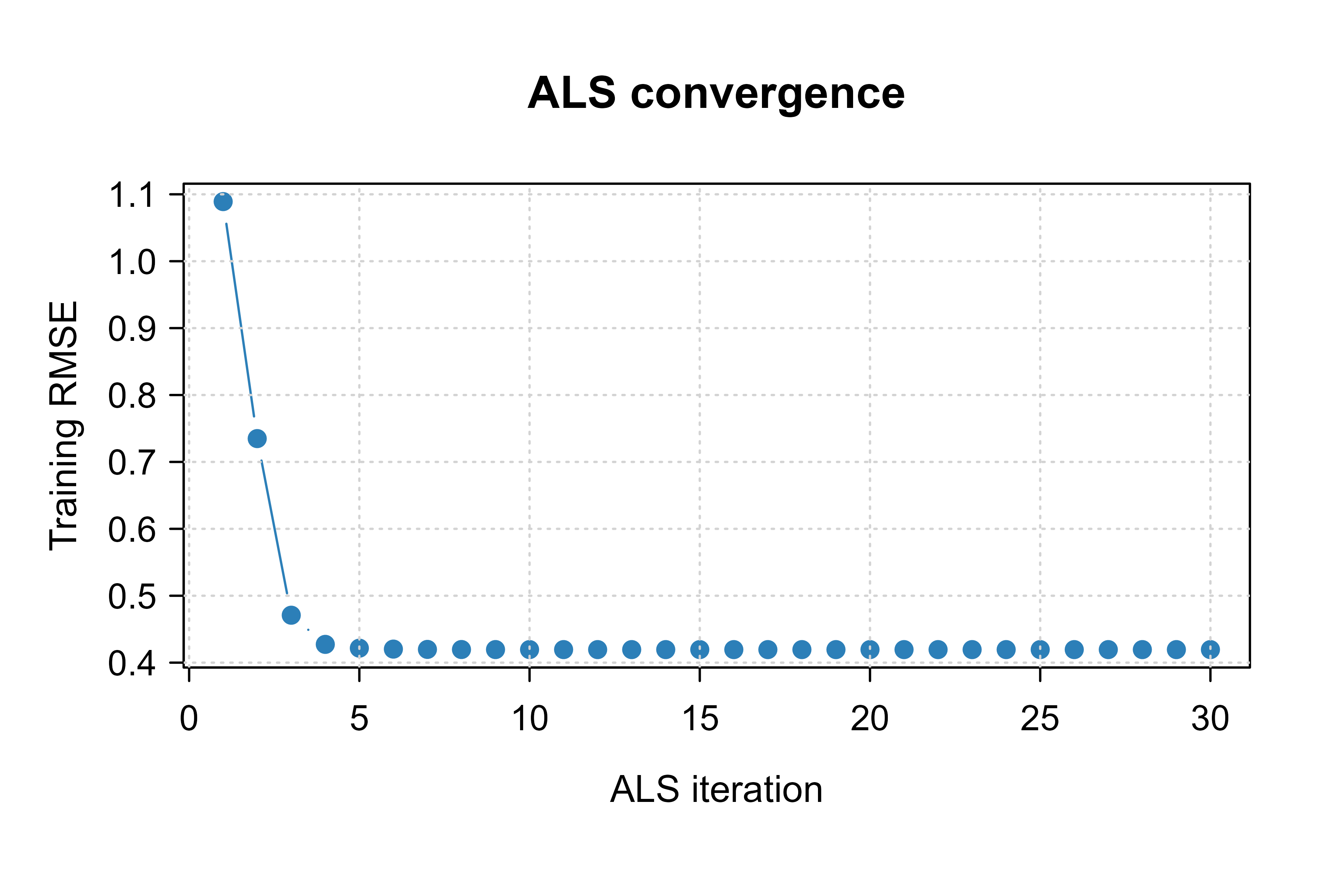
Figure 89.1 shows the ALS training RMSE falling and flattening over iterations, the visual signature of convergence. A curve that keeps dropping would mean we stopped too early; one that bottoms out and rises would warn of an instability.

plot(seq_along(als_model$rmse_hist), als_model$rmse_hist,
     type = "b", pch = 19, col = "#2c7fb8",
     xlab = "ALS iteration", ylab = "Training RMSE",
     main = "ALS convergence")
grid()

Figure 89.1: ALS training RMSE versus iteration. The error drops quickly in the first few sweeps and then flattens, indicating convergence of the alternating least-squares updates.

89.8.5 Test-set rating accuracy

Before ranking, we compare the two models on held-out rating prediction. We also include the simplest possible baseline, predicting the global mean for everything, to anchor the numbers.

rmse <- function(pred, truth, idx) {
  sqrt(mean((pred[idx] - truth[idx])^2))
}

global_mean <- mean(R_train, na.rm = TRUE)
pred_mean <- matrix(global_mean, m, n)

rmse_tbl <- data.frame(
  Model = c("Global mean", "Truncated SVD (imputed)", "Biased ALS"),
  `Test RMSE` = round(c(
    rmse(pred_mean, R_full, test_idx),
    rmse(pred_svd,  R_full, test_idx),
    rmse(pred_als,  R_full, test_idx)
  ), 3),
  check.names = FALSE
)
print(rmse_tbl)
#>                     Model Test RMSE
#> 1             Global mean     1.349
#> 2 Truncated SVD (imputed)     1.143
#> 3              Biased ALS     0.547

89.8.6 Generating top-N recommendations and ranking metrics

Rating error is only half the story. We now treat the models as rankers. For each user we define the relevant held-out items as those test entries whose true rating is at least \(4\) (a genuine “like”). We rank all of a user’s test items by predicted score, take the top \(N\), and compute precision@N, recall@N, and NDCG@N, averaged over users who have at least one relevant test item.

# Build per-user lists of (test item, true rating, predicted score)
test_pos <- which(matrix(FALSE, m, n) | FALSE) # placeholder
test_cells <- arrayInd(test_idx, c(m, n))
colnames(test_cells) <- c("user", "item")

dcg_at_k <- function(rel) {
  if (length(rel) == 0) return(0)
  sum((2^rel - 1) / log2(seq_along(rel) + 1))
}

ranking_metrics <- function(pred, N = 5, thresh = 4) {
  prec <- rec <- ndcg <- c()
  for (u in seq_len(m)) {
    rows <- test_cells[test_cells[, "user"] == u, , drop = FALSE]
    if (nrow(rows) < 2) next
    items <- rows[, "item"]
    truth <- R_full[cbind(u, items)]
    score <- pred[cbind(u, items)]
    rel_all <- as.integer(truth >= thresh)
    if (sum(rel_all) == 0) next
    ord <- order(score, decreasing = TRUE)
    topN <- head(ord, N)
    rel_top <- rel_all[topN]
    prec <- c(prec, sum(rel_top) / length(topN))
    rec  <- c(rec,  sum(rel_top) / sum(rel_all))
    # NDCG: gains in predicted order vs ideal order
    idcg <- dcg_at_k(sort(rel_all, decreasing = TRUE)[seq_len(min(N, length(rel_all)))])
    dcg  <- dcg_at_k(rel_top)
    ndcg <- c(ndcg, if (idcg > 0) dcg / idcg else 0)
  }
  c(precision = mean(prec), recall = mean(rec), ndcg = mean(ndcg))
}

N <- 5
rank_tbl <- rbind(
  `Global mean` = ranking_metrics(pred_mean, N),
  `Truncated SVD` = ranking_metrics(pred_svd, N),
  `Biased ALS` = ranking_metrics(pred_als, N)
)
rank_tbl <- round(rank_tbl, 3)
print(rank_tbl)
#>               precision recall  ndcg
#> Global mean       0.274  0.402 0.364
#> Truncated SVD     0.487  0.737 0.715
#> Biased ALS        0.622  0.914 0.949

rank_df <- data.frame(
  Model = rownames(rank_tbl),
  `Precision@5` = rank_tbl[, "precision"],
  `Recall@5` = rank_tbl[, "recall"],
  `NDCG@5` = rank_tbl[, "ndcg"],
  check.names = FALSE,
  row.names = NULL
)
knitr::kable(
  rank_df,
  caption = "Top-5 ranking quality on held-out test ratings. The global-mean baseline cannot personalize, so its ranking is effectively random within a user; the latent-factor models recover the structure and rank genuine likes higher."
)

Table 89.2: Top-5 ranking quality on held-out test ratings. The global-mean baseline cannot personalize, so its ranking is effectively random within a user; the latent-factor models recover the structure and rank genuine likes higher.

Model	Precision@5	Recall@5	NDCG@5
Global mean	0.274	0.402	0.364
Truncated SVD	0.487	0.737	0.715
Biased ALS	0.622	0.914	0.949

Table 89.2 reports the headline result: both latent-factor models beat the non-personalized global-mean baseline on every ranking metric, and biased ALS, which optimizes over observed entries rather than an imputed matrix, edges out the truncated SVD. The global-mean model assigns the same score to every item for a user, so its ordering carries no personal signal and its ranking metrics hover near what random ordering would give.

Note

Exact numbers depend on the seeds and the small problem size. The qualitative ordering, personalized factor models above the popularity baseline and ALS at or above imputed SVD, is the robust takeaway, and it matches what the literature reports on real data.

89.8.7 Reading off a user’s recommendations

Finally, the payoff: turning predicted scores into an actual list for one user, excluding items they have already rated in training.

recommend_for_user <- function(pred, u, R_train, N = 5) {
  already <- which(!is.na(R_train[u, ]))
  scores <- pred[u, ]
  scores[already] <- -Inf  # never recommend an already-seen item
  top <- order(scores, decreasing = TRUE)[seq_len(N)]
  data.frame(item = top, predicted_rating = round(pred[u, top], 2))
}

cat("Top-5 recommendations for user 1 (ALS model):\n")
#> Top-5 recommendations for user 1 (ALS model):
print(recommend_for_user(pred_als, u = 1, R_train = R_train, N = 5))
#>   item predicted_rating
#> 1   20             5.56
#> 2   70             5.51
#> 3  103             5.47
#> 4  119             5.08
#> 5   99             5.04

The function masks out items the user has already seen, then returns the highest-scoring remainder. In a production system this same step would also filter by availability, business rules, and diversity constraints before the list reaches the screen.

89.9 Practical guidance and pitfalls

A handful of lessons recur across deployments, and most of the costly mistakes are conceptual rather than algorithmic.

Start with the right baseline. The bias-only model \(\mu + b_u + b_i\) (no latent factors at all) is shockingly hard to beat and takes minutes to fit. Always report it; a fancy model that does not clearly beat it is not earning its complexity. Likewise, popularity is the baseline that matters for cold users, and many “improvements” evaporate once you compare against it honestly.

Mind the train/test split. Random hold-out leaks the future into the past: in reality you predict tomorrow from today, so evaluate with a temporal split when timestamps exist. And always remove already-consumed items from the candidate set before scoring; otherwise you reward the model for recommending things the user has obviously already chosen.

Regularize and tune \(k\). The number of latent factors \(k\) and the penalty \(\lambda\) are the two knobs that matter most. Too large a \(k\) with too little regularization memorizes the sparse observations and generalizes poorly; cross-validate both. The sparser the matrix, the smaller the \(k\) you can support.

Respect the feedback type. Explicit ratings and implicit counts are different problems (Section 89.5). Do not paste implicit data into an explicit model with zeros for “not seen.” If your data is clicks and plays, use a confidence-weighted or negative-sampling method.

Watch for feedback loops and popularity bias. A deployed recommender shapes the very data it later trains on: items it shows get clicked, so they accumulate more positive signal, so they get shown more. Left unchecked this collapses diversity and entrenches a popularity rich-get-richer dynamic. Inject exploration, monitor catalog coverage, and beware of evaluating offline on data that a previous version of the same system generated.

Warning

Offline metrics and online outcomes can disagree. A model that wins on held-out NDCG may lose on live engagement because the offline data was itself filtered by the old recommender, and because metrics like NDCG do not capture novelty, diversity, or long-term satisfaction. Treat offline evaluation as a screen, not a verdict; confirm with an A/B test.

Finally, scale shapes the algorithm choice. Neighborhood methods are simple and explainable but degrade on very sparse, very large matrices; matrix factorization scales better and generalizes through the latent space; in industry both are now often components inside a larger two-stage pipeline (a cheap candidate generator followed by a learned re-ranker, a setting taken up in the learning to rank chapter, Chapter 78). Table 89.1 and the demo above cover the foundations every such pipeline rests on.

89.10 Further reading

For the matrix-factorization view that defined the modern field, see Koren, Bell, and Volinsky (2009), “Matrix Factorization Techniques for Recommender Systems,” which distills the Netflix Prize lessons. The implicit-feedback formulation is from Hu, Koren, and Volinsky (2008), “Collaborative Filtering for Implicit Feedback Datasets.” For item-based collaborative filtering at scale, see Sarwar, Karypis, Konstan, and Riedl (2001), “Item-Based Collaborative Filtering Recommendation Algorithms,” and Linden, Smith, and York (2003) on Amazon’s item-to-item approach. The Bayesian Personalized Ranking objective for top-N ranking is Rendle, Freudenthaler, Gantner, and Schmidt-Thieme (2009). For ranking-quality measurement including NDCG, see Jarvelin and Kekalainen (2002). Comprehensive textbook treatments include Aggarwal (2016), “Recommender Systems: The Textbook,” and Ricci, Rokach, and Shapira (eds., 2015), “Recommender Systems Handbook.” Hastie, Tibshirani, and Friedman (2009), “The Elements of Statistical Learning,” gives the SVD and regularized-regression background the factorization models rest on.