| Method | Learns | Action space | Gradient variance | Bias | Update stability |
|---|---|---|---|---|---|
| Q-learning (value-based) | Action values Q | Discrete | n/a (no policy gradient) | Low (tabular) | Can be unstable with approximation |
| REINFORCE | Policy only | Discrete or continuous | Very high | Unbiased | Erratic |
| REINFORCE + baseline | Policy + value baseline | Discrete or continuous | High | Unbiased | Better |
| A2C (actor-critic) | Policy + critic | Discrete or continuous | Lower (bootstrapped) | Biased (TD) | Good |
| PPO (actor-critic) | Policy + critic | Discrete or continuous | Lower (bootstrapped) | Biased (TD) | Strong (clipped) |
67 Policy Gradient and Actor-Critic Methods
In the previous reinforcement learning chapters (Chapter 64, Chapter 66) the agent learned a value function and then read a policy off it: estimate \(Q(s, a)\), then act greedily. That detour through values is not the only way, and sometimes it is the wrong way. Suppose the best action in a state is not “the single highest-value choice” but “choose left \(70\%\) of the time and right \(30\%\).” A greedy reading of a value function cannot express that; it always commits to one action. Or suppose the action is a continuous quantity, such as a steering angle or a dosage, where taking a \(\max\) over actions means searching over an infinite set on every step. In these situations it is more natural to skip the value function as the object of interest and instead adjust the policy itself, nudging the probabilities of actions up or down according to how well they turned out.
That is the idea behind policy gradient methods. We write the policy as a parameterized function, \(\pi_\theta(a \mid s)\), with tunable parameters \(\theta\) (the weights of a small model or a neural network). We define a scalar objective: the expected return when the agent follows that policy. Then we do what the rest of this book does everywhere else, climb the objective by gradient ascent. The twist is that the thing we are differentiating involves an expectation over trajectories that the policy itself generates, so the gradient is not a textbook derivative of a fixed loss. The central result of this chapter, the policy gradient theorem, tells us how to compute that gradient from sampled experience.
Intuition
A policy gradient method does not ask “which action is best?” It asks “in which direction should I shift my action probabilities so that, on average, returns go up?” If an action led to a good outcome, make it more likely; if it led to a bad outcome, make it less likely. The math below is a precise, unbiased way of carrying out that simple instinct.
By the end of the chapter you will understand parameterized policies, the policy gradient theorem and its score-function derivation, the REINFORCE algorithm, why REINFORCE is noisy and how a baseline fixes it, the advantage function, the actor-critic family (with A2C as the concrete case), and the trust-region ideas behind TRPO and PPO that make these methods stable enough for production. A fully runnable base-R demonstration trains REINFORCE on a softmax-policy bandit and shows the average return climbing over training. This chapter sits naturally after the value-based reinforcement learning material and directly underpins the reinforcement learning from human feedback (RLHF) stage used to align large language models (Chapter 40), which is built on PPO.
67.1 Why parameterize the policy directly
Value-based methods such as Q-learning store or approximate \(Q(s, a)\) and act greedily. That works well when the action set is small and discrete and when a deterministic policy is acceptable. Policy-based methods earn their place in three situations.
The first is continuous or very large action spaces. Taking \(\arg\max_a Q(s, a)\) is cheap when there are four actions and impossible when the action is a real-valued vector. A parameterized policy can output the parameters of a distribution (for example, the mean and variance of a Gaussian over steering angles) and sample from it directly, with no maximization step.
The second is stochastic optimal policies. In games with hidden information, or any setting an adversary can exploit, the best policy is genuinely random. Rock-paper-scissors has a unique optimal policy: play each action one third of the time. A greedy value reader cannot represent that; a parameterized stochastic policy can.
The third is smoothness. Value-based methods can change the policy abruptly: a tiny change in estimated values can flip the \(\arg\max\) and swing behavior from one action to another. Policy gradients move the action probabilities continuously, which often makes learning more stable, though at the cost of higher variance in the gradient estimate.
When to use this
Reach for policy gradients when actions are continuous, when the optimal policy is stochastic, or when you want smooth policy updates and are willing to accept noisier gradients. If actions are few and discrete and a deterministic greedy policy is fine, value-based methods are usually more sample efficient. Actor-critic methods, introduced later, try to capture the benefits of both.
67.1.1 Parameterized policies
A parameterized policy is a function \(\pi_\theta(a \mid s)\) that gives the probability of action \(a\) in state \(s\), controlled by parameters \(\theta \in \mathbb{R}^d\). The only requirements are that it defines a valid probability distribution over actions for every state and that it is differentiable in \(\theta\). Two forms cover most cases.
For discrete actions, the softmax (or Gibbs) policy assigns each action a preference \(h_\theta(s, a)\) (a linear function of features, or the output of a network) and normalizes:
\[ \pi_\theta(a \mid s) = \frac{\exp\!\big(h_\theta(s, a)\big)}{\sum_{a'} \exp\!\big(h_\theta(s, a')\big)}. \]
For continuous actions, a common choice is a Gaussian policy whose mean \(\mu_\theta(s)\) (and possibly variance) is a function of the state:
\[ \pi_\theta(a \mid s) = \frac{1}{\sqrt{2\pi}\,\sigma}\exp\!\left(-\frac{(a - \mu_\theta(s))^2}{2\sigma^2}\right). \]
The quantity that appears throughout the theory is the gradient of the log-probability, \(\nabla_\theta \log \pi_\theta(a \mid s)\), called the score function.1 For the softmax policy with linear preferences \(h_\theta(s, a) = \theta^\top \phi(s, a)\), where \(\phi(s, a)\) is a feature vector, the score has a clean closed form:
\[ \nabla_\theta \log \pi_\theta(a \mid s) = \phi(s, a) - \sum_{a'} \pi_\theta(a' \mid s)\, \phi(s, a') = \phi(s, a) - \mathbb{E}_{a' \sim \pi_\theta}\big[\phi(s, a')\big]. \]
In words, the score is the feature vector of the action you took minus the average feature vector under the current policy. Pushing \(\theta\) along this direction makes the chosen action more probable; pushing against it makes it less probable.
67.1.2 Regularity assumptions
Before differentiating an expectation over a parameter-dependent distribution, it is worth stating what makes the operation legitimate. The score-function estimator and the policy gradient theorem rest on the following assumptions, which hold for the softmax and Gaussian policies above and for essentially any neural policy used in practice.
- Differentiability and positive support. For every \((s, a)\), the map \(\theta \mapsto \pi_\theta(a \mid s)\) is differentiable, and \(\pi_\theta(a \mid s) > 0\) wherever it is sampled, so that \(\log \pi_\theta(a \mid s)\) and its gradient \(\nabla_\theta \log \pi_\theta(a \mid s)\) exist. A deterministic policy violates this, which is why policy gradient in its basic form needs a stochastic policy.
- Dominated differentiation. There is an integrable envelope that lets us exchange \(\nabla_\theta\) and the integral (the dominated convergence theorem, or Leibniz’s rule). With finite action sets and bounded rewards this is automatic; with continuous actions it requires the usual measure-theoretic regularity, which Gaussian policies satisfy.
- Finite objective. Either episodes terminate almost surely, or \(\gamma < 1\) with bounded rewards \(|r_t| \le R_{\max}\), so that \(J(\theta) = \mathbb{E}[\sum_t \gamma^t r_t]\) is finite (it is bounded by \(R_{\max}/(1-\gamma)\)).
Warning
The positivity requirement is not a technicality. If the policy ever assigns probability exactly zero to an action it nonetheless takes (for example through a hard clip or a degenerate variance), the score \(\nabla_\theta \log \pi_\theta\) is undefined and the gradient estimate blows up. Continuous policies should keep \(\sigma\) bounded away from zero, and discrete policies should avoid saturating the softmax to exact zeros.
67.2 The objective and the policy gradient theorem
Let \(\tau = (s_0, a_0, r_0, s_1, a_1, r_1, \dots)\) denote a trajectory generated by following \(\pi_\theta\), and let \(R(\tau) = \sum_{t \ge 0} \gamma^t r_t\) be its discounted return, with discount \(\gamma \in [0, 1]\). The agent wants to maximize the expected return:
\[ J(\theta) = \mathbb{E}_{\tau \sim \pi_\theta}\big[ R(\tau) \big]. \]
We would like \(\nabla_\theta J(\theta)\) so we can ascend it. The difficulty is that the distribution we are averaging over, the trajectory distribution, depends on \(\theta\). We cannot simply move the gradient inside the expectation, because the expectation is itself a function of \(\theta\).
67.2.1 The score-function (log-derivative) trick
The trick that unlocks everything is an identity. For any differentiable distribution \(p_\theta(x)\),
\[ \nabla_\theta p_\theta(x) = p_\theta(x)\, \frac{\nabla_\theta p_\theta(x)}{p_\theta(x)} = p_\theta(x)\, \nabla_\theta \log p_\theta(x), \]
which uses \(\nabla \log p = (\nabla p)/p\). Apply it to the gradient of an expectation of any function \(f(x)\) that does not depend on \(\theta\):
\[ \nabla_\theta \mathbb{E}_{x \sim p_\theta}[f(x)] = \nabla_\theta \int p_\theta(x) f(x)\, dx = \int \nabla_\theta p_\theta(x)\, f(x)\, dx = \int p_\theta(x)\, \nabla_\theta \log p_\theta(x)\, f(x)\, dx, \]
which is itself an expectation:
\[ \nabla_\theta \mathbb{E}_{x \sim p_\theta}[f(x)] = \mathbb{E}_{x \sim p_\theta}\big[ f(x)\, \nabla_\theta \log p_\theta(x) \big]. \]
The gradient of an expectation became an expectation of a gradient, which we can estimate by sampling. This is the score-function estimator (also called the likelihood-ratio estimator, and in the deep learning literature the REINFORCE estimator).
67.2.2 Applying it to trajectories
The probability of a trajectory under \(\pi_\theta\) factorizes into the (unknown) environment dynamics and the (known) policy:
\[ p_\theta(\tau) = p(s_0) \prod_{t \ge 0} \pi_\theta(a_t \mid s_t)\, P(s_{t+1} \mid s_t, a_t). \]
Take the log and then the gradient with respect to \(\theta\). The initial-state term and the transition terms do not depend on \(\theta\), so they drop out, leaving only the policy terms:
\[ \nabla_\theta \log p_\theta(\tau) = \sum_{t \ge 0} \nabla_\theta \log \pi_\theta(a_t \mid s_t). \]
This is the key payoff: the gradient of the trajectory log-probability needs only the policy, not the unknown environment model. Substituting into the score-function estimator with \(f(\tau) = R(\tau)\) gives the policy gradient theorem in its trajectory form (Williams 1992; Sutton et al. 2000):
\[ \nabla_\theta J(\theta) = \mathbb{E}_{\tau \sim \pi_\theta}\!\left[ \left( \sum_{t \ge 0} \nabla_\theta \log \pi_\theta(a_t \mid s_t) \right) R(\tau) \right]. \]
Key idea
The policy gradient is an average of score functions weighted by returns. Each action’s log-probability is pushed up in proportion to the return of the trajectory it was part of. Good trajectories raise the probability of every action they contain; bad trajectories lower it. No model of the environment is required, because the dynamics canceled out of the gradient.
67.2.3 Causality: only future rewards matter
The form above is correct but wasteful. An action at time \(t\) cannot influence rewards collected before \(t\), so weighting \(\nabla_\theta \log \pi_\theta(a_t \mid s_t)\) by the full-trajectory return \(R(\tau)\) adds noise from rewards that have nothing to do with that action. Removing those terms (they have zero expectation against the score and so do not bias the estimate) gives the reward-to-go form:
\[ \nabla_\theta J(\theta) = \mathbb{E}_{\tau \sim \pi_\theta}\!\left[ \sum_{t \ge 0} \gamma^t\, \nabla_\theta \log \pi_\theta(a_t \mid s_t)\, G_t \right], \qquad G_t = \sum_{k \ge 0} \gamma^k r_{t+k}. \]
Here \(G_t\) is the return from step \(t\) onward, the reward-to-go. This is the form REINFORCE actually uses.
67.2.4 Why dropping the past is unbiased
The claim that past rewards can be discarded “because they have zero expectation against the score” deserves an actual proof, because it is the same argument that later justifies the baseline. Fix a time \(t\) and an earlier reward \(r_k\) with \(k < t\). We want to show
\[ \mathbb{E}_{\tau \sim \pi_\theta}\!\big[ \nabla_\theta \log \pi_\theta(a_t \mid s_t)\, r_k \big] = 0, \qquad k < t. \]
Condition on everything up to and including time \(t\) except the action \(a_t\), that is on the history \(\mathcal{H}_t = (s_0, a_0, \dots, s_t)\). The reward \(r_k\) is a function of \(\mathcal{H}_t\) alone (it was already realized), so it is constant given \(\mathcal{H}_t\). Using the tower rule,
\[ \mathbb{E}\big[ \nabla_\theta \log \pi_\theta(a_t \mid s_t)\, r_k \big] = \mathbb{E}\Big[ r_k\, \underbrace{\mathbb{E}\big[ \nabla_\theta \log \pi_\theta(a_t \mid s_t) \,\big|\, \mathcal{H}_t \big]}_{= \,0} \Big]. \]
The inner expectation is the expected score under \(a_t \sim \pi_\theta(\cdot \mid s_t)\), which is zero by the score identity proved below in Section 67.4 (the same \(\mathbb{E}_{a \sim \pi_\theta}[\nabla_\theta \log \pi_\theta(a \mid s)] = 0\)). Hence every cross term with \(k < t\) vanishes, and replacing \(R(\tau) = \sum_k \gamma^k r_k\) by the reward-to-go \(G_t\) changes nothing in expectation while discarding pure noise. This is the prototype of all policy gradient variance reduction: subtract anything that is conditionally independent of \(a_t\) given the state, and the estimator stays unbiased.
67.2.5 The state-distribution form
The trajectory form is the most direct route to a sampling estimator, but the policy gradient theorem is more often stated in terms of the discounted state-visitation distribution, which exposes the structure used in convergence proofs and in actor-critic theory. Define the (unnormalized) discounted state distribution under \(\pi_\theta\),
\[ d^{\pi_\theta}(s) = \sum_{t \ge 0} \gamma^t \, \Pr(s_t = s \mid s_0 \sim p_0,\, \pi_\theta), \]
the expected discounted number of visits to \(s\). Starting from the reward-to-go form and using \(\mathbb{E}[G_t \mid s_t = s, a_t = a] = Q^{\pi_\theta}(s, a)\) together with the fact that \(\nabla_\theta \log \pi_\theta(a_t \mid s_t)\) depends only on the current \((s_t, a_t)\), we can take the conditional expectation of \(G_t\) inside the sum:
\[ \nabla_\theta J(\theta) = \mathbb{E}_{\tau}\!\left[ \sum_{t \ge 0} \gamma^t\, \nabla_\theta \log \pi_\theta(a_t \mid s_t)\, Q^{\pi_\theta}(s_t, a_t) \right] = \sum_s d^{\pi_\theta}(s) \sum_a \pi_\theta(a \mid s)\, \nabla_\theta \log \pi_\theta(a \mid s)\, Q^{\pi_\theta}(s, a). \]
Rewriting \(\pi_\theta \nabla_\theta \log \pi_\theta = \nabla_\theta \pi_\theta\) gives the canonical statement (Sutton et al. 2000):
\[ \nabla_\theta J(\theta) = \sum_s d^{\pi_\theta}(s) \sum_a \nabla_\theta \pi_\theta(a \mid s)\, Q^{\pi_\theta}(s, a). \tag{67.1}\]
Note
The factor \(\gamma^t\) multiplying the score is frequently dropped in practical implementations of REINFORCE and actor-critic, so that all time steps are weighted equally rather than discounted by their position in the episode. This makes the implemented update a (slightly) biased estimate of Equation 67.1: it optimizes the undiscounted visitation-weighted objective rather than the discounted one. The bias is usually benign and the equal weighting often helps learning, but it is the reason published pseudocode and the strict theorem do not always match.
The state-distribution form makes one structural fact transparent: the gradient only ever requires \(Q^{\pi_\theta}\) (or an unbiased estimate of it), never the transition model \(P\), and the dependence of \(d^{\pi_\theta}\) on \(\theta\) does not contribute to the gradient. That second point is the genuinely surprising content of the theorem. Changing \(\theta\) changes which states are visited, yet the derivative of the visitation distribution drops out, leaving a clean expectation over states sampled from the current policy.
67.3 REINFORCE
REINFORCE (Williams 1992) is the direct Monte Carlo implementation of the policy gradient theorem. Run an episode under the current policy, compute the reward-to-go \(G_t\) at each step, and take a gradient ascent step using the sample estimate of the gradient. The per-episode update is
\[ \theta \leftarrow \theta + \alpha \sum_{t \ge 0} \nabla_\theta \log \pi_\theta(a_t \mid s_t)\, G_t, \]
with learning rate \(\alpha > 0\). The algorithm is appealingly simple and makes no assumptions about the environment beyond being able to sample from it.
Warning
REINFORCE is unbiased but high variance. Because \(G_t\) is a Monte Carlo estimate over an entire (random) future, a single lucky or unlucky episode can produce a large, misleading gradient. In practice plain REINFORCE learns slowly and erratically, which is the entire motivation for the variance-reduction techniques in the next section.
67.4 Variance reduction with a baseline
The fix for the variance problem is a baseline. Subtract from each return a quantity \(b(s_t)\) that depends on the state but not on the action taken:
\[ \nabla_\theta J(\theta) = \mathbb{E}_{\tau \sim \pi_\theta}\!\left[ \sum_{t \ge 0} \nabla_\theta \log \pi_\theta(a_t \mid s_t)\, \big( G_t - b(s_t) \big) \right]. \]
Subtracting the baseline does not change the expected gradient. The reason is that the expected score is zero: for any state,
\[ \mathbb{E}_{a \sim \pi_\theta}\big[ \nabla_\theta \log \pi_\theta(a \mid s) \big] = \sum_a \pi_\theta(a \mid s)\, \frac{\nabla_\theta \pi_\theta(a \mid s)}{\pi_\theta(a \mid s)} = \nabla_\theta \sum_a \pi_\theta(a \mid s) = \nabla_\theta 1 = 0. \]
Because \(b(s_t)\) does not depend on \(a_t\), its contribution is \(b(s_t)\) times this zero expectation, so the estimator stays unbiased for any choice of baseline. What the baseline does change is the variance. The variance-minimizing baseline is close to the expected return from that state, which is exactly the state value \(V^\pi(s_t)\). Using the value as the baseline makes the weight \(G_t - V^\pi(s_t)\) measure how much better the actual outcome was than what the policy expected on average.
67.4.1 The variance-minimizing baseline
It is worth deriving exactly which constant baseline minimizes variance, because the answer is not simply \(V^\pi(s)\) but a score-weighted version of it, and the distinction explains why a separately learned value function is a good but not optimal baseline. Consider a single state \(s\) and a scalar component of the gradient, with score \(g = \nabla_\theta \log \pi_\theta(a \mid s)\) and return \(G\). For a constant baseline \(b\) the per-sample estimator is \(g\,(G - b)\). Its expectation is fixed (the baseline term vanishes), so minimizing variance is the same as minimizing the second moment
\[ \mathcal{L}(b) = \mathbb{E}\big[\, g^2 (G - b)^2 \,\big]. \]
Differentiating and setting to zero,
\[ \frac{d \mathcal{L}}{d b} = -2\, \mathbb{E}\big[\, g^2 (G - b) \,\big] = 0 \quad\Longrightarrow\quad b^\star = \frac{\mathbb{E}\big[\, g^2 G \,\big]}{\mathbb{E}\big[\, g^2 \,\big]}. \tag{67.2}\]
The variance-optimal baseline is the return weighted by the squared score, a magnitude-weighted average return, not the plain average return \(V^\pi(s) = \mathbb{E}[G]\). When the score magnitude \(g^2\) is roughly uncorrelated with \(G\), the two coincide and \(b^\star \approx V^\pi(s)\), which is why the state value is the standard, near-optimal choice. The exact optimum Equation 67.2 is rarely implemented because estimating it well is harder than estimating \(V^\pi\), and the residual gain is small.
How much variance does a baseline remove?
With \(A = G - V^\pi(s)\) the advantage and using the centered estimator \(g\,A\), the per-sample variance is \(\mathbb{E}[g^2 A^2]\). Because the advantage has zero conditional mean, \(\mathbb{E}[A^2 \mid s]\) is the conditional variance of the return, which is typically far smaller than \(\mathbb{E}[G^2 \mid s]\) whenever the state’s return level \(V^\pi(s)\) is large. The baseline removes exactly the \(V^\pi(s)^2\) contribution that the raw estimator \(gG\) carries, which is the dominant term in any problem where returns are large and similar across actions in a state.
Intuition
Without a baseline, an action that yields a return of \(+100\) in a state where every action yields about \(+100\) still gets its probability pushed up hard, even though it was not special. The baseline recenters the signal: only the part of the return that exceeds the state’s typical value carries information about whether the action was better or worse than usual. Subtracting the mean does not bias the direction of the push, it just removes a large, uninformative common component and shrinks the noise.
67.4.2 The advantage function
The recentered quantity \(G_t - V^\pi(s_t)\) is an estimate of the advantage function,
\[ A^\pi(s, a) = Q^\pi(s, a) - V^\pi(s), \]
the amount by which taking action \(a\) in state \(s\) and then following \(\pi\) beats the average action in that state. Positive advantage means “better than usual, do more of this”; negative means “worse than usual, do less.” The policy gradient written with the advantage is the form most modern algorithms target:
\[ \nabla_\theta J(\theta) = \mathbb{E}_{\tau \sim \pi_\theta}\!\left[ \sum_{t \ge 0} \nabla_\theta \log \pi_\theta(a_t \mid s_t)\, A^\pi(s_t, a_t) \right]. \]
67.4.3 Compatible function approximation
When the critic is itself a learned approximation \(\hat{A}_w(s, a)\) rather than the true advantage, substituting it into the policy gradient generally introduces bias. There is, however, a precise condition under which the substitution is exact. Suppose the critic is linear in the policy’s own score features,
\[ \hat{A}_w(s, a) = w^\top \nabla_\theta \log \pi_\theta(a \mid s), \]
and \(w\) is fitted by minimizing the mean squared error \(\mathbb{E}[(\hat{A}_w(s,a) - A^{\pi_\theta}(s,a))^2]\) under the on-policy state-action distribution. The first-order optimality condition for that regression is
\[ \mathbb{E}\big[ \nabla_\theta \log \pi_\theta(a \mid s)\,(\hat{A}_w(s,a) - A^{\pi_\theta}(s,a)) \big] = 0, \]
which is exactly the condition needed for \(\mathbb{E}[\nabla_\theta \log \pi_\theta \cdot \hat{A}_w] = \mathbb{E}[\nabla_\theta \log \pi_\theta \cdot A^{\pi_\theta}] = \nabla_\theta J(\theta)\). This is the compatible function approximation theorem (Sutton et al. 2000): a critic that is linear in the score features and fitted by least squares yields an unbiased policy gradient. It is also the formal bridge to natural policy gradients, where this same \(w\) turns out to be the natural gradient direction \(F(\theta)^{-1} \nabla_\theta J(\theta)\) with \(F(\theta)\) the Fisher information of the policy.
67.5 Actor-critic methods
REINFORCE with a value baseline needs an estimate of \(V^\pi\). The cleanest way to get one is to learn it alongside the policy, and that is the actor-critic idea. Two parameterized functions are trained together:
- The actor is the policy \(\pi_\theta(a \mid s)\), updated in the direction of the policy gradient.
- The critic is a value function \(V_w(s)\) with its own parameters \(w\), trained to predict returns and used to compute the advantage that weights the actor’s update.
Instead of waiting for a full Monte Carlo return \(G_t\), the critic lets us bootstrap: replace \(G_t\) with the one-step temporal-difference (TD) target \(r_t + \gamma V_w(s_{t+1})\) (Chapter 66). The TD error
\[ \delta_t = r_t + \gamma V_w(s_{t+1}) - V_w(s_t) \]
is a low-variance, biased estimate of the advantage \(A^\pi(s_t, a_t)\). The actor and critic are updated each step:
\[ w \leftarrow w + \alpha_w\, \delta_t\, \nabla_w V_w(s_t), \qquad \theta \leftarrow \theta + \alpha_\theta\, \delta_t\, \nabla_\theta \log \pi_\theta(a_t \mid s_t). \]
Key idea
The critic trades variance for bias. Monte Carlo returns are unbiased but noisy; bootstrapped TD targets are biased (the critic is imperfect) but far less noisy. Actor-critic methods sit on the bias-variance spectrum between pure REINFORCE (all Monte Carlo) and pure dynamic programming (all bootstrap), and that middle ground is usually where learning is fastest.
67.5.1 n-step returns and generalized advantage estimation
The one-step TD error \(\delta_t\) minimizes variance but maximizes bias, since it leans entirely on the imperfect critic. The full Monte Carlo return \(G_t\) does the opposite. Between them lies a one-parameter family. The \(n\)-step advantage estimate
\[ \hat{A}^{(n)}_t = \sum_{l=0}^{n-1} \gamma^l r_{t+l} + \gamma^n V_w(s_{t+n}) - V_w(s_t) \]
uses \(n\) real rewards and then bootstraps. Small \(n\) is low-variance and high-bias; large \(n\) approaches Monte Carlo. Generalized advantage estimation (GAE; Schulman et al. 2016) avoids choosing \(n\) by taking an exponentially weighted average of all \(n\)-step estimates. Writing \(\delta_t = r_t + \gamma V_w(s_{t+1}) - V_w(s_t)\) for the one-step TD error, one can telescope the \(n\)-step advantages into a sum of TD errors, \(\hat{A}^{(n)}_t = \sum_{l=0}^{n-1} \gamma^l \delta_{t+l}\), and the \(\lambda\)-weighted average collapses to a clean geometric series:
\[ \hat{A}^{\text{GAE}(\gamma, \lambda)}_t = (1 - \lambda) \sum_{n \ge 1} \lambda^{n-1} \hat{A}^{(n)}_t = \sum_{l \ge 0} (\gamma \lambda)^l\, \delta_{t+l}. \tag{67.3}\]
The parameter \(\lambda \in [0, 1]\) is an explicit bias-variance dial: \(\lambda = 0\) recovers the one-step TD advantage \(\delta_t\) (low variance, high bias), and \(\lambda = 1\) recovers the Monte Carlo advantage \(G_t - V_w(s_t)\) (unbiased, high variance). Values around \(\lambda = 0.95\) to \(0.97\) are the standard default. The GAE recursion \(\hat{A}_t = \delta_t + \gamma\lambda\,\hat{A}_{t+1}\) computes Equation 67.3 in a single backward pass over a trajectory and is what PPO implementations use to form \(\hat{A}_t\).
67.5.2 A2C
Advantage Actor-Critic (A2C) is the standard synchronous form. It runs several environment copies in parallel, collects a short batch of transitions from each, computes advantages (often with multi-step or generalized advantage estimation), and applies one synchronized update to a shared actor and critic. Running many environments at once decorrelates the data (which stabilizes the gradient, much as a replay buffer does for value-based methods) and keeps hardware busy. A2C is the synchronous counterpart of the earlier asynchronous A3C (Mnih et al. 2016); the synchronous version is simpler and usually performs at least as well.
Table 67.1 compares the methods discussed so far along the dimensions that matter when choosing one.
67.6 Trust regions and PPO
Plain policy gradient ascent has a subtle hazard: the natural step size in parameter space does not correspond to a sensible step size in policy space. A small change in \(\theta\) can produce a large change in the action distribution, and a single overlarge step can collapse the policy to something terrible from which it never recovers. Because the data the agent collects next is generated by the current policy, a bad step poisons all future learning. This is the central failure mode that trust-region methods address.
67.6.1 The surrogate objective and the monotonic improvement bound
The trust-region machinery rests on an exact identity for the difference in performance between two policies. For any policies \(\pi\) and \(\pi_{\text{old}}\), the performance difference lemma (Kakade and Langford 2002) states
\[ J(\pi) - J(\pi_{\text{old}}) = \mathbb{E}_{s \sim d^{\pi}}\, \mathbb{E}_{a \sim \pi(\cdot \mid s)}\big[ A^{\pi_{\text{old}}}(s, a) \big]. \tag{67.4}\]
This is exact but not directly usable, because the expectation is over \(d^{\pi}\), the visitation distribution of the new policy we have not run yet. The surrogate objective replaces \(d^{\pi}\) with the old policy’s visitation \(d^{\pi_{\text{old}}}\), which we can sample, and corrects the action distribution with an importance-sampling ratio:
\[ L_{\pi_{\text{old}}}(\pi) = \mathbb{E}_{s \sim d^{\pi_{\text{old}}}}\, \mathbb{E}_{a \sim \pi_{\text{old}}}\!\left[ \frac{\pi(a \mid s)}{\pi_{\text{old}}(a \mid s)}\, A^{\pi_{\text{old}}}(s, a) \right]. \]
The surrogate agrees with the true objective to first order at \(\pi = \pi_{\text{old}}\) (both value and gradient match), so a small improvement in \(L\) is a small improvement in \(J\). TRPO makes this rigorous with a bound: the true improvement is at least the surrogate improvement minus a penalty proportional to the worst-case KL divergence between the policies,
\[ J(\pi) \ge L_{\pi_{\text{old}}}(\pi) - C\, \max_s \mathrm{KL}\!\big(\pi_{\text{old}}(\cdot \mid s)\,\|\,\pi(\cdot \mid s)\big), \qquad C = \frac{4 \gamma \max_{s,a} |A^{\pi_{\text{old}}}(s,a)|}{(1-\gamma)^2}. \tag{67.5}\]
Maximizing the right-hand side of Equation 67.5 guarantees monotonic improvement of the true objective, which is the theoretical justification for the entire trust-region family. In practice the KL penalty coefficient \(C\) from the bound is far too conservative (it forces tiny steps), so TRPO instead imposes KL as a hard constraint with a tunable threshold and PPO replaces it with clipping, trading the guarantee for usable step sizes.
Trust Region Policy Optimization (TRPO; Schulman et al. 2015) makes the policy improvement explicit and constrains how far the new policy may move from the old one, measured by the Kullback-Leibler (KL) divergence between the two action distributions. It maximizes a surrogate objective built from the probability ratio
\[ \rho_t(\theta) = \frac{\pi_\theta(a_t \mid s_t)}{\pi_{\theta_{\text{old}}}(a_t \mid s_t)}, \]
subject to a constraint that the average KL divergence stays below a small threshold. The constraint is what keeps each update inside a region where the surrogate is trustworthy, hence “trust region.”
Proximal Policy Optimization (PPO; Schulman et al. 2017) keeps the trust-region spirit but replaces the hard KL constraint with a clipped objective that is far simpler to implement and works with ordinary first-order optimizers. PPO maximizes
\[ L^{\text{CLIP}}(\theta) = \mathbb{E}_t\Big[ \min\big( \rho_t(\theta)\, \hat{A}_t,\ \operatorname{clip}(\rho_t(\theta),\, 1 - \epsilon,\, 1 + \epsilon)\, \hat{A}_t \big) \Big], \]
where \(\hat{A}_t\) is an estimated advantage and \(\epsilon\) (typically around \(0.1\) to \(0.2\)) sets the clip width. The clip removes any incentive to push the probability ratio far beyond \(1 \pm \epsilon\), so even if the raw gradient wants a huge step, the objective flattens and the update stays modest.
The \(\min\) and the asymmetry between positive and negative advantage are easy to misread, so it is worth tracing the four cases. When \(\hat{A}_t > 0\) the objective is \(\hat{A}_t \min(\rho_t, 1+\epsilon)\): increasing \(\rho_t\) helps until it reaches \(1+\epsilon\), after which the gradient is zero, so a good action can be made more likely but only up to the cap. When \(\hat{A}_t < 0\) the objective is \(\hat{A}_t \max(\rho_t, 1-\epsilon)\) (the \(\min\) of two negatives picks the larger ratio term): decreasing \(\rho_t\) helps until it reaches \(1-\epsilon\), then flattens. The \(\min\) is what makes the bound pessimistic, it always takes the more conservative of the clipped and unclipped surrogate. One consequence is that the clip is one-sided: it never penalizes the agent for being too cautious, only for stepping too far, so PPO still requires a finite number of epochs per data batch (typically 3 to 10) rather than optimizing the surrogate to convergence, which would let the ratio escape the clip region between gradient steps.
PPO is not the surrogate’s global optimum
Clipping zeros the gradient outside \([1-\epsilon, 1+\epsilon]\) but does not undo a step that already left that region (for example from an earlier minibatch in the same epoch). This is why PPO implementations also monitor the empirical KL divergence and stop the epoch early if it exceeds a target. The clip is a soft, local safeguard, not a hard constraint like TRPO’s.
Note
PPO is the workhorse behind reinforcement learning from human feedback (RLHF) for large language models. In that setting the policy is the language model, the action is the next token, and the reward comes from a learned model of human preference. The clipping in PPO is what keeps the fine-tuned model from drifting catastrophically far from the pretrained one in a single update. The chapter on large language models (Chapter 40) builds directly on these ideas.
67.7 A runnable REINFORCE demo in base R
To make the mechanics concrete we train REINFORCE on a softmax-policy bandit, the simplest setting in which the full policy gradient machinery applies. There is a single state, so the policy is a distribution over \(K\) actions controlled by preference parameters \(\theta \in \mathbb{R}^K\). Each action \(a\) pays a stochastic reward with unknown mean \(\mu_a\); the agent never sees the means, only sampled rewards. This strips away the environment dynamics and lets us watch the score-function update, the baseline, and the rising return curve in isolation.
The policy is the softmax over preferences, \(\pi_\theta(a) = e^{\theta_a} / \sum_{a'} e^{\theta_{a'}}\). For this policy the score function for the sampled action \(a\) is \(\nabla_\theta \log \pi_\theta(a) = \mathbf{1}_a - \pi_\theta\), where \(\mathbf{1}_a\) is the indicator vector for action \(a\). We use a running average of observed rewards as the baseline \(b\), so each update nudges \(\theta\) by \(\alpha\,(r - b)\,(\mathbf{1}_a - \pi_\theta)\). The hyperparameters are collected in Table 67.2.
| Hyperparameter | Value | Role |
|---|---|---|
| Number of actions (K) | 4 | Size of the action set |
| True reward means | 0.2, 0.5, 1.0, 1.6 | Hidden payoffs; action 4 is best |
| Reward noise (sd) | 1.0 | Stochasticity of each reward |
| Learning rate (alpha) | 0.1 | Step size for gradient ascent |
| Baseline | running mean reward | Variance reduction (subtracted from reward) |
| Training steps | 2000 | Number of policy-gradient updates |
| Random seed | 42 | Reproducibility |
The code below implements the loop. Each step samples an action from the current softmax policy, draws a noisy reward, forms the advantage reward - baseline, and updates the preferences along the score function.
Show code
set.seed(42)

K          <- 4                       # number of actions
mu         <- c(0.2, 0.5, 1.0, 1.6)   # hidden mean rewards (action 4 best)
reward_sd  <- 1.0                     # reward noise
alpha      <- 0.1                     # learning rate
n_steps    <- 2000                    # number of updates

softmax <- function(theta) {
  z <- theta - max(theta)             # subtract max for numerical stability
  ex <- exp(z)
  ex / sum(ex)
}

theta    <- rep(0, K)                 # preferences: uniform policy at start
baseline <- 0                         # running-mean baseline
returns  <- numeric(n_steps)          # reward received at each step
probs_best <- numeric(n_steps)        # probability mass on the best action

for (t in seq_len(n_steps)) {
  p <- softmax(theta)                 # current policy
  a <- sample.int(K, size = 1, prob = p)        # sample an action
  r <- rnorm(1, mean = mu[a], sd = reward_sd)   # observe a noisy reward

  # Score function for softmax: indicator(a) - p
  grad_logp     <- -p
  grad_logp[a]  <- grad_logp[a] + 1

  # REINFORCE update with baseline: theta <- theta + alpha * (r - b) * score
  theta <- theta + alpha * (r - baseline) * grad_logp

  # Update running-mean baseline
  baseline <- baseline + (r - baseline) / t

  returns[t]    <- r
  probs_best[t] <- p[which.max(mu)]
}

# Smooth the noisy per-step reward with a trailing moving average
moving_avg <- function(x, w = 50) {
  n <- length(x)
  out <- rep(NA_real_, n)
  cs <- cumsum(x)
  for (i in seq_len(n)) {
    lo <- max(1, i - w + 1)
    out[i] <- (cs[i] - if (lo > 1) cs[lo - 1] else 0) / (i - lo + 1)
  }
  out
}
avg_return <- moving_avg(returns, w = 50)

final_policy <- softmax(theta)
cat("Final policy (action probabilities):\n")
#> Final policy (action probabilities):
print(round(final_policy, 3))
#> [1] 0.000 0.001 0.001 0.998
cat(sprintf("\nProbability on best action (action %d): %.3f\n",
            which.max(mu), final_policy[which.max(mu)]))
#>
#> Probability on best action (action 4): 0.998
The printed policy concentrates probability on action 4, the action with the highest hidden mean, even though the agent only ever saw noisy samples and never the means themselves. Figure 67.1 shows the learning curves: the left panel is the moving-average reward climbing toward the best action’s mean of \(1.6\), and the right panel is the probability mass the policy places on the best action rising from \(0.25\) (uniform over four actions) toward \(1\).
Show code
op <- par(mfrow = c(1, 2), mar = c(4, 4, 3, 1))

plot(avg_return, type = "l", col = "steelblue", lwd = 2,
     xlab = "Training step", ylab = "Average reward (50-step window)",
     main = "Average return increases")
abline(h = max(mu), lty = 2, col = "grey50")

plot(probs_best, type = "l", col = "darkorange", lwd = 2,
     ylim = c(0, 1),
     xlab = "Training step", ylab = "P(best action)",
     main = "Policy concentrates on best action")
abline(h = 1 / K, lty = 3, col = "grey50")   # uniform starting probability

par(op)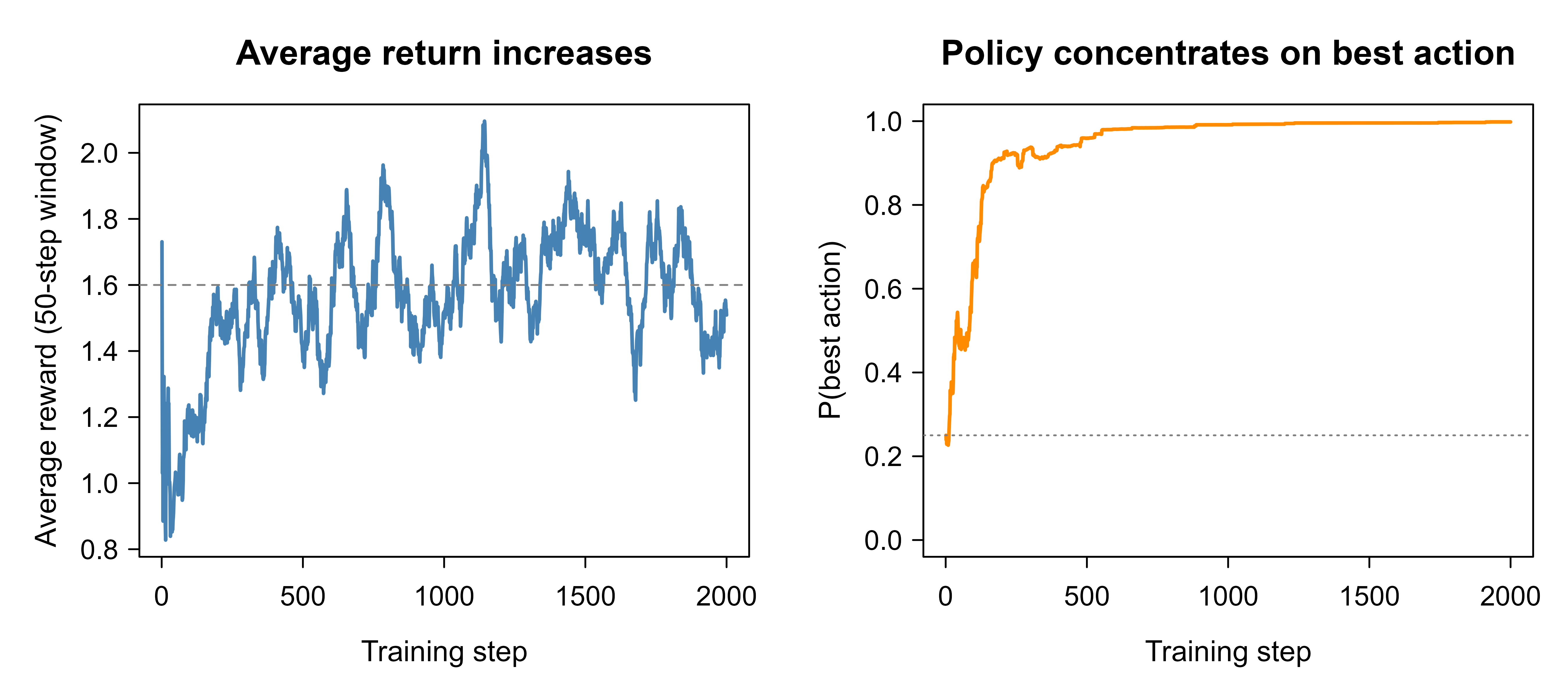
The whole story of policy gradients is on this one figure. The score function pushed probability toward actions that paid more than the baseline and away from actions that paid less, and over two thousand small steps that local rule found the best action without ever computing a value function or taking a maximum over actions.
Note
The baseline matters even in this trivial problem. With rewards centered near \(+1\), an estimator without a baseline would push up the probability of whatever action it just sampled simply because the raw reward is positive, regardless of whether that action was actually better than the alternatives. Subtracting the running-mean baseline turns the signal into “better or worse than typical,” which is what makes the policy discriminate among actions rather than inflating all of them.
67.8 Deep-network policies
For anything beyond a toy problem the actor and critic are neural networks rather than a handful of preferences, and the gradient is computed by automatic differentiation. The sketch below shows the shape of an A2C-style update with the torch package for R (Chapter 92). It is shown for orientation only and is not run as part of this book.
Show code
library(torch)

# Actor and critic as small multilayer perceptrons sharing the state input.
make_mlp <- function(in_dim, out_dim) {
  nn_sequential(
    nn_linear(in_dim, 64), nn_tanh(),
    nn_linear(64, 64),     nn_tanh(),
    nn_linear(64, out_dim)
  )
}

state_dim  <- 4    # e.g. CartPole observation
n_actions  <- 2

actor  <- make_mlp(state_dim, n_actions)   # outputs action logits
critic <- make_mlp(state_dim, 1)           # outputs state value V(s)

opt <- optim_adam(c(actor$parameters, critic$parameters), lr = 3e-4)

# One synchronous A2C update from a batch of transitions.
# states: (N x state_dim), actions: (N), returns: (N) discounted reward-to-go
a2c_update <- function(states, actions, returns) {
  logits <- actor(states)
  values <- critic(states)$squeeze(2)

  logp_all  <- nnf_log_softmax(logits, dim = 2)
  logp_take <- logp_all$gather(2, actions$unsqueeze(2)$to(dtype = torch_long()))$squeeze(2)

  advantage <- (returns - values)$detach()      # stop critic grad into actor

  actor_loss  <- -(logp_take * advantage)$mean()        # policy gradient
  critic_loss <- nnf_mse_loss(values, returns)          # fit the critic
  entropy     <- -(logp_all$exp() * logp_all)$sum(dim = 2)$mean()

  loss <- actor_loss + 0.5 * critic_loss - 0.01 * entropy   # entropy bonus

  opt$zero_grad()
  loss$backward()
  nn_utils_clip_grad_norm_(c(actor$parameters, critic$parameters), 0.5)
  opt$step()
  invisible(loss$item())
}
The structure mirrors the base-R demo exactly. The actor loss is the negative log-probability of the taken action weighted by the advantage (gradient ascent on the policy objective), the critic loss fits the value function by regression onto returns, and the small entropy bonus discourages the policy from collapsing to a deterministic choice too early. Swapping the Monte Carlo returns for a clipped surrogate objective turns this into PPO.
67.9 Convergence, complexity, and failure modes
The policy gradient is an unbiased (or, with a critic, low-bias) stochastic gradient of a smooth but nonconvex objective, so the classical stochastic-approximation guarantees apply: under the Robbins-Monro step-size conditions \(\sum_t \alpha_t = \infty\) and \(\sum_t \alpha_t^2 < \infty\), REINFORCE and actor-critic converge to a stationary point of \(J(\theta)\) almost surely (Sutton et al. 2000; Konda and Tsitsiklis 2000). Two-timescale actor-critic schemes require the critic to be updated faster than the actor (\(\alpha_w / \alpha_\theta \to \infty\)) so the critic tracks \(V^{\pi_\theta}\) and the actor sees an approximately correct advantage. The guarantee is only to a stationary point, not a global optimum, since \(J\) is nonconvex in \(\theta\) for any nontrivial policy class.
On rates, generic first-order analysis gives \(\mathbb{E}\|\nabla_\theta J\|^2 = O(1/\sqrt{T})\) after \(T\) stochastic gradient steps, the standard nonconvex SGD rate, with the constant governed by the gradient variance, which is where baselines and critics earn their keep. Stronger results exist under structure: for softmax policies with exact gradients, policy gradient enjoys an \(O(1/T)\) rate, and with entropy regularization a linear \(O(c^T)\) rate, because the regularized objective satisfies a gradient-domination (Polyak-Lojasiewicz) inequality. Natural policy gradient improves the dependence on the policy parameterization by preconditioning with the Fisher information, which makes the update invariant to reparameterization and is the theoretical ancestor of TRPO and PPO.
The dominant failure modes follow directly from the theory. High variance of the score-function estimator scales with the reward magnitude and the trajectory horizon \(1/(1-\gamma)\), so long-horizon, large-reward problems are the hardest and most need baselines, GAE, and reward normalization. Premature determinism is the second: as the policy sharpens, exploration collapses and the agent stops sampling the actions whose advantages it would need to keep improving, which is why an entropy bonus is standard. The third is destructive updates, the motivation for trust regions: because the next batch of data is drawn from the current policy, a single overlarge step on the nonconvex landscape can move the policy to a region of state space where the critic is uninformative, and learning does not recover. On-policy sample inefficiency is the fourth and most fundamental: every gradient step strictly needs fresh trajectories from the current policy, so policy gradient methods typically need orders of magnitude more environment interaction than off-policy value-based methods that reuse a replay buffer.
67.10 A numerical check of the score-function identities
Before relying on these estimators it is reassuring to confirm two of the load-bearing claims directly: that the score-function estimator is unbiased for the true gradient, and that subtracting a baseline leaves the expectation unchanged while shrinking the variance. We do this on the softmax bandit, where the true gradient is available in closed form. For a single state the objective is \(J(\theta) = \sum_a \pi_\theta(a)\,\mu_a\), and since \(\nabla_\theta J = \sum_a \pi_\theta(a)\,(\mathbf{1}_a - \pi_\theta)\,\mu_a\) we can compare the Monte Carlo estimator against it.
Show code
set.seed(7)
K   <- 4
mu  <- c(0.2, 0.5, 1.0, 1.6)          # true action means
th  <- c(0.3, -0.1, 0.4, 0.0)         # an arbitrary (non-uniform) policy

softmax <- function(theta) {
  z <- theta - max(theta); ex <- exp(z); ex / sum(ex)
}
p <- softmax(th)

# Closed-form gradient of J(theta) = sum_a pi(a) mu_a
score_mat <- diag(K) - matrix(p, K, K, byrow = TRUE)   # rows: 1_a - p
true_grad <- as.numeric(t(score_mat) %*% (p * mu))

# Monte Carlo score-function estimator, with and without a baseline.
N        <- 2e5
acts     <- sample.int(K, N, replace = TRUE, prob = p)
rewards  <- rnorm(N, mean = mu[acts], sd = 1.0)
scores   <- score_mat[acts, , drop = FALSE]            # N x K score vectors
baseline <- sum(p * mu)                                # E[reward] = V

est_nobase <- colMeans(scores * rewards)
est_base   <- colMeans(scores * (rewards - baseline))

# Variance of one coordinate (action 4) of the estimator, per sample.
var_nobase <- var(scores[, 4] * rewards)
var_base   <- var(scores[, 4] * (rewards - baseline))

cat("True gradient:        ", round(true_grad, 4), "\n")
#> True gradient:         -0.1717 -0.0579 0.0617 0.1678
cat("MC estimate (no base):", round(est_nobase, 4), "\n")
#> MC estimate (no base): -0.1718 -0.0571 0.0611 0.1678
cat("MC estimate (baseline):", round(est_base, 4), "\n")
#> MC estimate (baseline): -0.1712 -0.0575 0.0609 0.1678
cat(sprintf("Per-sample variance, coord 4:  no base = %.3f,  baseline = %.3f\n",
            var_nobase, var_base))
#> Per-sample variance, coord 4:  no base = 0.491,  baseline = 0.228
Both Monte Carlo estimates match the closed-form gradient to sampling error, confirming that the baseline does not bias the estimator, and the per-sample variance is substantially smaller with the baseline subtracted, confirming that it is doing its job.
67.11 Practical guidance and pitfalls
Policy gradient methods are powerful but finicky, and most of the trouble is predictable. The points below collect the lessons that save the most time, roughly in the order you will meet them.
Start with a baseline, always. Plain REINFORCE without a baseline is a teaching device, not a tool; the variance is high enough that learning is slow and unreliable. A state-value baseline (or the running-mean baseline in the demo) costs almost nothing and helps immediately.
Normalize advantages within a batch. Subtracting the batch mean and dividing by the batch standard deviation of the advantages makes the effective step size far more stable across problems and reward scales. This single trick removes a great deal of hyperparameter sensitivity.
Keep an entropy bonus early. Without it the policy can become nearly deterministic before it has explored enough, then it stops sampling the actions it would need to discover something better. A small entropy term in the objective keeps the policy stochastic long enough to explore.
Mind the learning rates. Actor and critic usually need different step sizes, and the actor in particular is sensitive: too large and the policy can collapse in one update, the failure mode that motivated trust-region methods. If a run diverges suddenly after looking healthy, suspect the actor step size first.
Watch the reward scale. Because the gradient is the score weighted by returns, the magnitude of the reward directly scales the gradient. Rewards in the thousands or in tiny fractions both cause trouble; rescaling rewards or normalizing returns fixes it.
Evaluate without exploration noise. Training return includes the randomness of the stochastic policy. To measure real progress, periodically run a near-greedy version (lower the temperature, or take the most probable action) and report that.
Reach for PPO when stability matters. For most practical discrete or continuous control problems, and for RLHF, PPO is the sensible default: it captures the variance reduction of actor-critic and the stability of trust regions with a simple, robust objective. Plain REINFORCE and A2C are worth understanding and are fine on small problems, but PPO is what tends to survive contact with a real task.
Tip
Seed several runs and compare. Variance across random seeds is large for policy gradient methods, large enough that a single run can mislead you about whether a change helped. Reporting the spread across seeds, not a single curve, is standard practice for a reason.
In one line: policy gradient methods optimize a parameterized policy directly by ascending the expected return, the policy gradient theorem makes that gradient an estimable expectation of score functions weighted by returns (or advantages), baselines and critics cut its variance, and trust-region ideas (PPO) keep the updates safe enough to scale all the way up to aligning large language models.
67.12 Further reading
- Sutton and Barto (2018), Reinforcement Learning: An Introduction (2nd ed.). The standard textbook; Chapter 13 covers policy gradient methods, REINFORCE, baselines, and actor-critic in full.
- Williams (1992), Simple statistical gradient-following algorithms for connectionist reinforcement learning. The original REINFORCE estimator.
- Sutton, McAllester, Singh, and Mansour (2000), Policy gradient methods for reinforcement learning with function approximation. The policy gradient theorem with function approximation.
- Konda and Tsitsiklis (2000), Actor-critic algorithms. The foundational analysis of actor-critic methods, including the two-timescale convergence argument.
- Kakade and Langford (2002), Approximately optimal approximate reinforcement learning. The performance difference lemma and the conservative policy iteration bound that TRPO and PPO build on.
- Kakade (2002), A natural policy gradient. The natural gradient view and its connection to compatible function approximation.
- Mnih et al. (2016), Asynchronous methods for deep reinforcement learning. Introduces A3C, the asynchronous precursor to A2C.
- Schulman et al. (2015), Trust region policy optimization. The TRPO algorithm and trust-region motivation.
- Schulman et al. (2017), Proximal policy optimization algorithms. The PPO clipped objective used widely in control and in RLHF.
- Schulman et al. (2016), High-dimensional continuous control using generalized advantage estimation. The GAE advantage estimator used with actor-critic methods.
The name comes from statistics, where the score is the gradient of the log-likelihood with respect to the parameters. It is the same object that appears in maximum-likelihood estimation, which is why fitting a policy by policy gradient looks so much like weighted maximum likelihood: each action is treated as an observation weighted by how good its outcome was.↩︎