Imagine you want to predict the price of a house from its features (number of rooms, neighborhood income, distance to work, and so on). A single regression tree (Chapter 8) is easy to read but usually too crude. A forest of many trees (Chapter 13) predicts well but gives you a single point estimate with no honest sense of how uncertain that estimate is. Bayesian Additive Regression Trees, or BART (Sparapani, Spanbauer, and McCulloch 2021), try to give you the best of both: the flexibility of a sum of many small trees, plus a full probability distribution over the prediction so you can attach uncertainty to every number you report.
This chapter introduces BART from intuition first, then states the algorithm precisely, and finally walks through worked examples in R using the BART package. By the end you should understand why BART is often called a “good out-of-the-box” method, how its three main settings (number of trees, number of iterations, and burn-in) work, and how to read its output, including convergence checks, variable importance, and partial dependence plots.
When to use this
BART is a strong default when you want flexible, nonlinear regression or classification with little tuning, and you also want uncertainty intervals around predictions. It pairs naturally with the tree-based and ensemble ideas you have already seen.
BART sits in the same family as the methods in the chapters on bagging (Chapter 10), random forests (Chapter 13), and boosting (Chapter 11), and it borrows one key idea from each. As in bagging and random forests, every tree is built using randomness rather than a single deterministic greedy search. As in boosting, every tree tries to capture the part of the signal that the rest of the model has not yet explained.1
14.1 The model: a sum of trees
The core idea is simple to state. Instead of one big tree, BART uses a sum of many small trees, and each tree contributes a small piece of the final prediction.
Let \(K\) be the number of regression trees, and let \(B\) be the number of MCMC iterations for which the BART algorithm will be run. Let \(\hat{f}_k^b(x)\) represent the prediction at \(x\) for the \(k\)-th regression tree used in the \(b\)-th iteration. The prediction from a single iteration is the sum of all \(K\) trees in that iteration:
\[
\hat{f}^b(x) = \sum_{k=1}^K \hat{f}_k^b(x), b = 1, \dots, B
\]
Key idea
No single tree has to be good on its own. Each tree is deliberately kept small (a “weak learner”), and the prediction comes from adding many of them together. Keeping each tree small is the main guard against overfitting.
14.1.1 The probabilistic model and likelihood
The algorithmic description above hides a fully specified Bayesian model, which we now write out precisely because every step of the sampler (the random perturbations, the “favoring” of good fits, even the burn-in) is a consequence of it. Following Chipman, George, and McCulloch (2010), the original BART paper, we write a single tree as a pair \((T_k, M_k)\), where \(T_k\) encodes the tree topology, that is, the internal splitting rules (each a variable index and a split value) and the leaf structure, and \(M_k = \{\mu_{k1}, \dots, \mu_{kb_k}\}\) collects the scalar parameters stored in its \(b_k\) terminal nodes. Writing \(g(x; T_k, M_k)\) for the function that drops \(x\) down tree \(T_k\) and returns the leaf value, the model is the sum of trees plus Gaussian noise,
Before fitting, the continuous response is centered and scaled (the BART package rescales \(y\) to the interval \([-0.5, 0.5]\)). This is not cosmetic: it is what lets the same default prior hyperparameters work across data sets with wildly different units, which is a large part of why BART is “out of the box.”
14.1.2 The prior: regularization made explicit
What stops a sum of \(K = 200\) trees from interpolating the data is the prior, not the likelihood. BART places independent priors on the trees and on the variance, and assumes the trees are mutually independent and independent of \(\sigma\):
The factor \((1+d)^{-\beta}\) makes deeper splits polynomially less likely, so the prior concentrates on shallow “stumpy” trees. The BART defaults are \(\alpha = 0.95\) and \(\beta = 2\), under which the prior probability of a tree of depth \(0, 1, 2, 3\) being a single node, then splitting once, twice, and so on, puts the overwhelming mass on trees with one or two levels: with \(\beta = 2\) the split probabilities are \(0.95\) at the root, \(0.95/4 \approx 0.24\) at depth 1, \(0.95/9 \approx 0.11\) at depth 2. Given that a node splits, the splitting variable is drawn uniformly over available predictors and the split point uniformly over its available values.
Leaf-value prior \(p(\mu_{kj} \mid T_k)\). Each leaf parameter gets a conjugate Gaussian prior centered at zero,
Centering at zero is sensible because the response has been centered, and the \(K\) trees share the signal additively, so each leaf should contribute only a small piece. The variance \(\sigma_\mu^2\) is set so that the prior on the sum, \(E[Y \mid x] = \sum_k g(x; T_k, M_k)\), which by independence has variance \(K \sigma_\mu^2\), places most of its mass on the observed range of \(y\). Concretely, Chipman, George, and McCulloch (2010) choose \(\sigma_\mu = 0.5/(c\sqrt{K})\) on the rescaled response, where \(c\) (default \(c = 2\)) is the number of prior standard deviations of the centered response that should fit in the half-range \(0.5\). The crucial consequence is the \(1/\sqrt{K}\) shrinkage: adding more trees automatically shrinks each leaf, so \(K\) controls model complexity gently rather than catastrophically.
Error-variance prior \(p(\sigma^2)\). A conjugate inverse-gamma prior is used, written as a scaled inverse chi-squared,
The degrees of freedom \(\nu\) (default \(3\)) controls the tail, and \(\lambda\) is calibrated from the data so that a chosen prior quantile \(q\) (default \(0.90\)) of \(\sigma\) falls at a rough overestimate of the noise level, typically the residual standard deviation \(\hat\sigma\) from a least-squares fit of \(y\) on \(X\). This anchors the variance prior to the data’s scale while keeping it weakly informative.
14.1.3 Starting point
We need a place to begin the chain. In the first iteration, all trees are initialized to have a single root node with \(\hat{f}_k^1(x) = (1/nK)\sum_{i=1}^n y_i\), which is the mean of the response values divided by the total number of trees. Splitting the overall mean equally across the \(K\) trees means that when we add the trees back up, we recover exactly the mean response:
BART starts from the simplest possible prediction, “guess the average for everyone,” and then lets the trees gradually carve out structure from there.
14.1.4 Updating one tree at a time using partial residuals
In each later iteration, BART updates each of the \(K\) trees, one at a time. The trick that makes this work is the partial residual: when we are about to update tree \(k\), we temporarily remove its contribution and ask how far off the rest of the model is. Whatever the other trees fail to explain is exactly what tree \(k\) should try to capture.
Concretely, in the \(b\)-th iteration, to update the \(k\)-th tree, we subtract from each response value the predictions from all but the \(k\)-th tree to obtain a partial residual:
\[
r_i = y_i - \sum_{k'<k} \hat{f}_{k'}^b (x_i) - \sum_{k'>k} \hat{f}_{k'}^{b-1}(x_i), i = 1, \dots, n
\]
Notice the bookkeeping in the two sums: trees with index \(k' < k\) have already been updated in the current iteration \(b\), so we use their fresh values, while trees with \(k' > k\) have not been touched yet this round, so we use their values from the previous iteration \(b-1\).
Here is the step that makes BART Bayesian rather than just another boosting scheme. Instead of fitting a brand new tree to this partial residual, BART randomly chooses a perturbation to the tree from the previous iteration (\(\hat{f}_k^{b-1}\)) out of a set of possible perturbations (this is where MCMC comes in), favoring ones that improve the fit to the partial residual.2 There are two components to this perturbation, which we apply together:
change the structure of the tree by adding or pruning branches, and
change the prediction value stored in each terminal (leaf) node of the tree.
Note
Because we perturb the existing tree rather than regrowing it from scratch, no single update can move the model very far. This deliberate timidity is what keeps BART from chasing noise.
14.1.5 Deriving the Bayesian backfitting update
The phrase “favoring perturbations that improve the fit” is, made precise, a Gibbs sampler that draws each unknown from its full conditional given everything else, a scheme Chipman, George, and McCulloch (2010) call Bayesian backfitting. We now derive each conditional. Condition throughout on \(\sigma^2\) and on all trees other than the \(k\)-th, and let \(r = (r_1, \dots, r_n)\) be the partial residual defined above. By construction \(r_i = g(x_i; T_k, M_k) + \varepsilon_i\), so the \(k\)-th tree sees a clean single-tree regression problem with response \(r\). The full conditional for \((T_k, M_k)\) depends on the others only through \(r\):
BART draws this in two steps: first \(T_k \mid r, \sigma^2\) with \(M_k\) integrated out, then \(M_k \mid T_k, r, \sigma^2\).
Step 1: integrate out the leaves to get the marginal likelihood. Because the Gaussian leaf prior Equation 14.5 is conjugate to the Gaussian likelihood, we can integrate \(M_k\) out in closed form, which is what makes the tree move feasible. The tree partitions the \(n\) residuals into the leaves; let leaf \(j\) contain the index set with \(n_j\) residuals, sum \(S_j = \sum_{i \in \text{leaf } j} r_i\), and let the leaf parameters be independent across leaves. For a single leaf with \(n_j\) observations \(r_i \sim N(\mu, \sigma^2)\) and prior \(\mu \sim N(0, \sigma_\mu^2)\), completing the square in \(\mu\) gives the marginal
The full tree marginal likelihood is the product of Equation 14.8 over leaves \(j = 1, \dots, b_k\). This scalar is the quantity that “scores” a candidate tree.
Step 2: the leaf posterior. Given the tree, the leaves are conditionally independent and each is a standard conjugate normal-normal update. For leaf \(j\),
The posterior mean is a precision-weighted average of the leaf’s residual mean \(S_j/n_j\) and the prior mean \(0\), so leaves with few observations are shrunk hard toward zero. This is the exact mechanism behind “each tree contributes a small piece.”
We can confirm Equation 14.9 numerically with a tiny simulation: draw residuals in one leaf, then check that the analytic posterior mean and variance match a brute-force Monte Carlo evaluation of the unnormalized posterior \(\prod_i N(r_i;\mu,\sigma^2)\,N(\mu;0,\sigma_\mu^2)\).
Show code
set.seed(1)nj<-8; sigma2<-1.5; sigma_mu2<-0.4r<-rnorm(nj, mean =1.2, sd =sqrt(sigma2))# residuals in one leafSj<-sum(r)# analytic posterior from eq-BART.qmd-mu-postpost_var<-1/(nj/sigma2+1/sigma_mu2)post_mean<-post_var*(Sj/sigma2)# brute-force normalization over a fine grid of mumu<-seq(-3, 3, length.out =20001)logpost<-sapply(mu, function(m)sum(dnorm(r, m, sqrt(sigma2), log =TRUE))+dnorm(m, 0, sqrt(sigma_mu2), log =TRUE))w<-exp(logpost-max(logpost)); w<-w/sum(w)num_mean<-sum(mu*w)num_var<-sum((mu-num_mean)^2*w)c(analytic_mean =post_mean, numeric_mean =num_mean, analytic_var =post_var, numeric_var =num_var)#> analytic_mean numeric_mean analytic_var numeric_var #> 0.9266370 0.9266370 0.1276596 0.1276596
The analytic and numerical values agree to several digits, confirming the conjugate update.
Step 3: the Metropolis-Hastings move on tree structure. The tree topology \(T_k\) has no conjugate form, so it is updated with a Metropolis-Hastings step using Equation 14.8 as the marginalized target. A move \(T_k \to T_k^\star\) is proposed from a kernel \(q(\cdot \mid \cdot)\) that picks among GROW (split a leaf into two), PRUNE (collapse two sibling leaves into one), CHANGE (alter a split rule), and SWAP (exchange rules of a parent and child). The proposal is accepted with probability
The middle factor is where the depth penalty \(p_{\text{split}}(d)\) from Equation 14.4 enters: a GROW move that deepens the tree must overcome the prior’s reluctance to split, which is precisely the regularization. Because the likelihood ratio uses the marginalized form, only the leaves touched by the move (the split or pruned node) actually change the score, so each MH evaluation is cheap, \(O(n_j)\) in the affected leaves rather than \(O(n)\).
Step 4: update \(\sigma^2\). After all \(K\) trees are refreshed, form the full residual \(e_i = y_i - \sum_k g(x_i; T_k, M_k)\). Conjugacy of Equation 14.6 gives the inverse-gamma full conditional
which is the trace plotted in the convergence diagnostic later in this chapter. One full sweep over Equation 14.10, Equation 14.9, and Equation 14.11 is one MCMC iteration \(b\).
14.1.6 Collecting the output
After running the chain, the output of BART is not one model but a whole collection of prediction models, one per iteration:
\[
\hat{f}^b(x) = \sum_{k =1}^K \hat{f}_k^b (x) , b = 1, \dots, B
\]
Early iterations are unreliable because the chain has not yet settled down, so we discard the first \(L\) iterations as a burn-in period and average over the rest:
The payoff of the Bayesian framing appears here: because each retained iteration is a posterior sample, we are not limited to the average. We can use the spread of the posterior samples to get distributional estimates of the predictions, that is, credible intervals rather than just point predictions.
Tip
When someone asks “how confident are you in this prediction?”, BART has a direct answer: look at the variability of \(\hat{f}^b(x)\) across the retained iterations.
14.2 The BART algorithm
Putting the pieces together, the full procedure is summarized below, following (James et al. 2013) Alg 8.3. The outer loop walks through MCMC iterations, the middle loop walks through the \(K\) trees, and the inner loop computes the partial residual for each observation before perturbing the current tree.
For \(i = 1, \dots , n\), compute the current partial residual (\(r_i\))
Fit a new tree \(\hat{f}_k^b(x)\) to \(r_i\) by randomly perturbing the \(k\)-th tree from the previous iteration, \(\hat{f}_k^{b-1}(x)\) (favor perturbations that improve the fit)
Compute the mean after \(L\) burn-in samples \(\hat{f}(x) = \frac{1}{B - L} \sum_{b = L +1}^B \hat{f}^b (x)\)
A few remarks make the algorithm easier to reason about. Step 3.1.2 prevents overfitting because it limits how hard we fit the data in each iteration: a single perturbation can only nudge a tree a little. The individual trees are kept quite small on purpose; limiting tree size is another guard against overfitting, since very large trees would memorize the training data. And, as noted above, each time we randomly perturb a tree to fit the residuals we are effectively drawing a new tree from a posterior distribution.
When we use BART, we have to specify three quantities:
the number of trees \(K\),
the number of iterations \(B\), and
the number of burn-in iterations \(L\).
In practice these are easy to set. We typically choose large values such as \(B = 1000\) and \(K = 200\), and a moderate value such as \(L = 100\). Because these defaults work well across many problems, BART is a good out-of-the-box tool that needs minimal tuning.
Warning
The defaults are robust, but they are not free. With \(K = 200\) trees and \(B = 1000\) iterations, BART does a lot of computation, and runtime grows with the number of observations and predictors. If a run is slow, the thinning trick shown later in this chapter can help.
14.2.1 Choosing the hyperparameters
Beyond the three loop counts \((K, B, L)\), the model is governed by the prior hyperparameters derived above. The following table collects them, their BART defaults, and the effect of moving each.
Hyperparameter
Role
Default
Effect of increasing
\(K\) (ntree)
number of trees
200
more flexible mean, more shrinkage per leaf via \(\sigma_\mu \propto 1/\sqrt K\)
The single most useful tuning knob is \(c\) (k in the package): values in \([1, 3]\) trade flexibility for smoothness, and cross-validating over \(\{1, 2, 3\}\) alongside \(K \in \{50, 200\}\) recovers most of the achievable gain. Increasing \(K\) rarely hurts accuracy (the per-leaf shrinkage compensates), so the practical limit on \(K\) is compute, not overfitting. If predictions look too wiggly, raise \(c\) or \(\beta\); if BART underfits a known sharp nonlinearity, lower them.
Diagnostics checklist
Always plot the sigma trace (Figure 14.2) and confirm it has stabilized past burn-in. For a second check, run two or more chains from different seeds and confirm their posterior means agree. Effective sample size on \(\sigma\) and on a few held-out predictions tells you whether thinning or a longer chain is needed.
14.2.2 Theoretical properties and connections
Bias-variance and the role of \(K\). Each tree is a weak learner with small variance but high bias; summing \(K\) of them, with leaf variance scaled as \(\sigma_\mu^2 \propto 1/K\), keeps the prior variance of the sum \(K\sigma_\mu^2\) constant while letting the ensemble represent rich interactions. This is the additive-model analogue of boosting’s bias reduction, but achieved by averaging over a posterior rather than a single greedy path.
Posterior consistency and rates. BART is not merely a heuristic. Ročková and Pas (2020) prove that, with a tree prior of the form Equation 14.4 and appropriately chosen \(\sigma_\mu\), the BART posterior concentrates around the true regression function at the near-minimax rate \(n^{-s/(2s + p)}\) (up to log factors) for \(s\)-Hölder smooth functions of \(p\) inputs, and adapts to unknown smoothness and to low-dimensional structure (sparsity in the active predictors). The shrinkage prior on tree depth is essential to these guarantees: without it the posterior would overfit.
Connections. BART is a Bayesian sibling of gradient boosting (Chapter 11): both fit a sum of trees to evolving residuals, but boosting takes one forward greedy pass with a fixed shrinkage step, whereas BART resamples every tree from its full conditional, producing a posterior. The leaf shrinkage Equation 14.9 is exactly ridge-type regularization applied per leaf, and the marginal likelihood Equation 14.8 is the same evidence used in Bayesian linear regression, here applied locally within each leaf. Like random forests (Chapter 13), BART averages over many trees, but the averaging is over MCMC draws governed by a likelihood rather than over bootstrap resamples.
Failure modes. BART can mix slowly when predictors are highly collinear (many near-equivalent splits) or when \(n\) is large and the posterior over tree structures is multimodal; trace plots that drift are the symptom. It assumes additive Gaussian noise in Equation 14.1, so heavy tails or strong heteroscedasticity violate the model and distort the credible intervals (variants such as heteroscedastic BART and DART address these). Extrapolation beyond the range of the training predictors reverts toward the leaf means and gives untrustworthy intervals, because the trees can only partition observed support.
14.3 Worked example: predicting Boston housing prices
We start with the example from (James et al. 2013, Ch 8.3), which predicts the median home value medv in the Boston data from all other predictors. The workflow is the familiar one: split into training and test sets, fit the model on the training data, then measure error on the held-out test set. The function gbart is the BART package’s general-purpose fitter for a continuous response.
Show code
library(BART)library(ISLR2)library(tree)set.seed(1)train<-sample(1:nrow(ISLR2::Boston), nrow(ISLR2::Boston)/2)# tree.boston <- tree(medv ~ ., ISLR2::Boston, subset = train)x<-ISLR2::Boston[,1:12]y<-ISLR2::Boston[,"medv"]xtrain<-x[train,]ytrain<-y[train]xtest<-x[-train,]ytest<-y[-train]bartfit<-gbart(xtrain, ytrain, x.test =xtest)#> *****Calling gbart: type=1#> *****Data:#> data:n,p,np: 253, 12, 253#> y1,yn: 0.213439, -5.486561#> x1,x[n*p]: 0.109590, 20.080000#> xp1,xp[np*p]: 0.027310, 7.880000#> *****Number of Trees: 200#> *****Number of Cut Points: 100 ... 100#> *****burn,nd,thin: 100,1000,1#> *****Prior:beta,alpha,tau,nu,lambda,offset: 2,0.95,0.795495,3,3.71636,21.7866#> *****sigma: 4.367914#> *****w (weights): 1.000000 ... 1.000000#> *****Dirichlet:sparse,theta,omega,a,b,rho,augment: 0,0,1,0.5,1,12,0#> *****printevery: 100#> #> MCMC#> done 0 (out of 1100)#> done 100 (out of 1100)#> done 200 (out of 1100)#> done 300 (out of 1100)#> done 400 (out of 1100)#> done 500 (out of 1100)#> done 600 (out of 1100)#> done 700 (out of 1100)#> done 800 (out of 1100)#> done 900 (out of 1100)#> done 1000 (out of 1100)#> time: 5s#> trcnt,tecnt: 1000,1000# test erroryhat.bart<-bartfit$yhat.test.meanmean((ytest-yhat.bart)^2)#> [1] 15.97434# how many times each variable appeared in the colelction of treesord<-order(bartfit$varcount.mean, decreasing =T)bartfit$varcount.mean[ord]#> lstat nox tax rm rad chas indus ptratio age dis #> 21.638 21.458 20.900 20.725 20.627 20.102 19.640 19.083 18.736 15.417 #> zn crim #> 15.146 11.891
Two pieces of output are worth reading carefully. The first, the mean squared error on the test set, is the headline accuracy number: smaller is better, and on this split BART is competitive with or better than boosting and random forests. The second, varcount.mean, counts how many times each variable appeared in the collection of trees, averaged over iterations. Variables that show up more often are the ones BART relied on more heavily, so this gives a quick, model-based ranking of variable importance.
Note
Variable appearance counts are a useful first look at importance, but they are not the whole story. A variable can be used many times in shallow splits without changing predictions much. The partial dependence plot later in this chapter shows the direction and shape of a variable’s effect, which counts alone cannot.
14.4 Worked example: the package authors’ walkthrough
The next sequence follows the example from the package’s own authors (Sparapani, Spanbauer, and McCulloch 2021). To keep things visual, it restricts attention to two predictors so we can plot everything. The response and predictors are:
y = medv, the median value of owner-occupied homes,
x1 = rm, the average number of rooms, and
x2 = lstat, the percent of the population that is lower status.
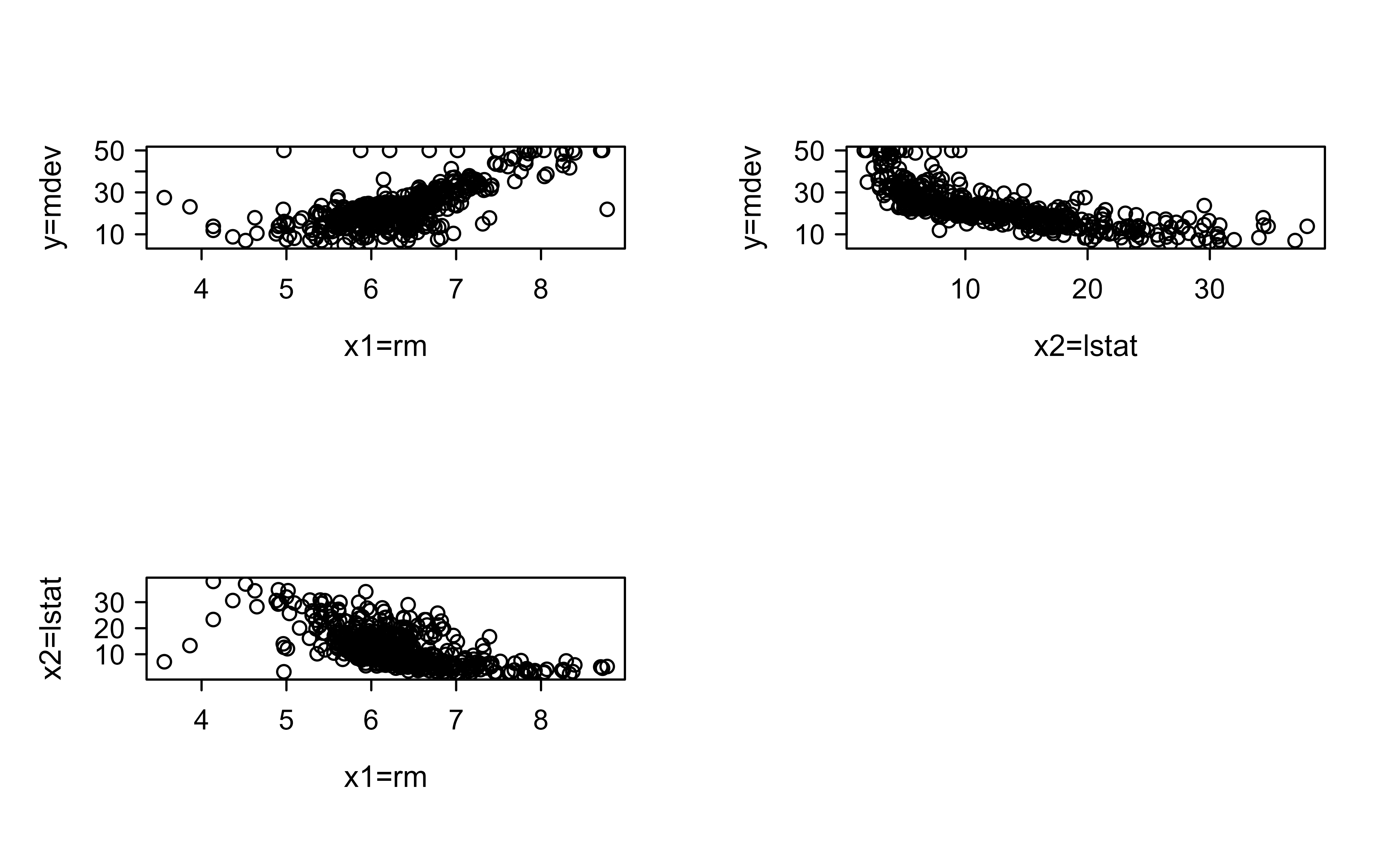
Before fitting anything, it pays to look at the raw relationships. Figure 14.1 shows each predictor against the response and the two predictors against each other.
Figure 14.1: Scatterplots of the raw Boston data: median home value against average number of rooms (x1=rm), median home value against percent lower status (x2=lstat), and the two predictors against each other.
The plots already hint at what any good model should recover: home value rises with the number of rooms and falls as the lower-status percentage increases, and the two predictors are themselves negatively related. We now fit BART and see whether it captures these patterns.
Here we use wbart, the function for a continuous (weighted) response, and we ask for nd = 200 posterior draws after a burn-in of burn = 50 draws.3
Show code
library("BART")set.seed(99)nd<-200# number of posterior drawsburn<-50# use wbart for continuous varaiblespost<-wbart(x, y, nskip =burn, ndpost =nd)#> *****Into main of wbart#> *****Data:#> data:n,p,np: 506, 2, 0#> y1,yn: 1.467194, -10.632806#> x1,x[n*p]: 6.575000, 7.880000#> *****Number of Trees: 200#> *****Number of Cut Points: 100 ... 100#> *****burn and ndpost: 50, 200#> *****Prior:beta,alpha,tau,nu,lambda: 2.000000,0.950000,0.795495,3.000000,5.979017#> *****sigma: 5.540257#> *****w (weights): 1.000000 ... 1.000000#> *****Dirichlet:sparse,theta,omega,a,b,rho,augment: 0,0,1,0.5,1,2,0#> *****nkeeptrain,nkeeptest,nkeeptestme,nkeeptreedraws: 200,200,200,200#> *****printevery: 100#> *****skiptr,skipte,skipteme,skiptreedraws: 1,1,1,1#> #> MCMC#> done 0 (out of 250)#> done 100 (out of 250)#> done 200 (out of 250)#> time: 1s#> check counts#> trcnt,tecnt,temecnt,treedrawscnt: 200,0,0,200
14.4.1 Checking convergence
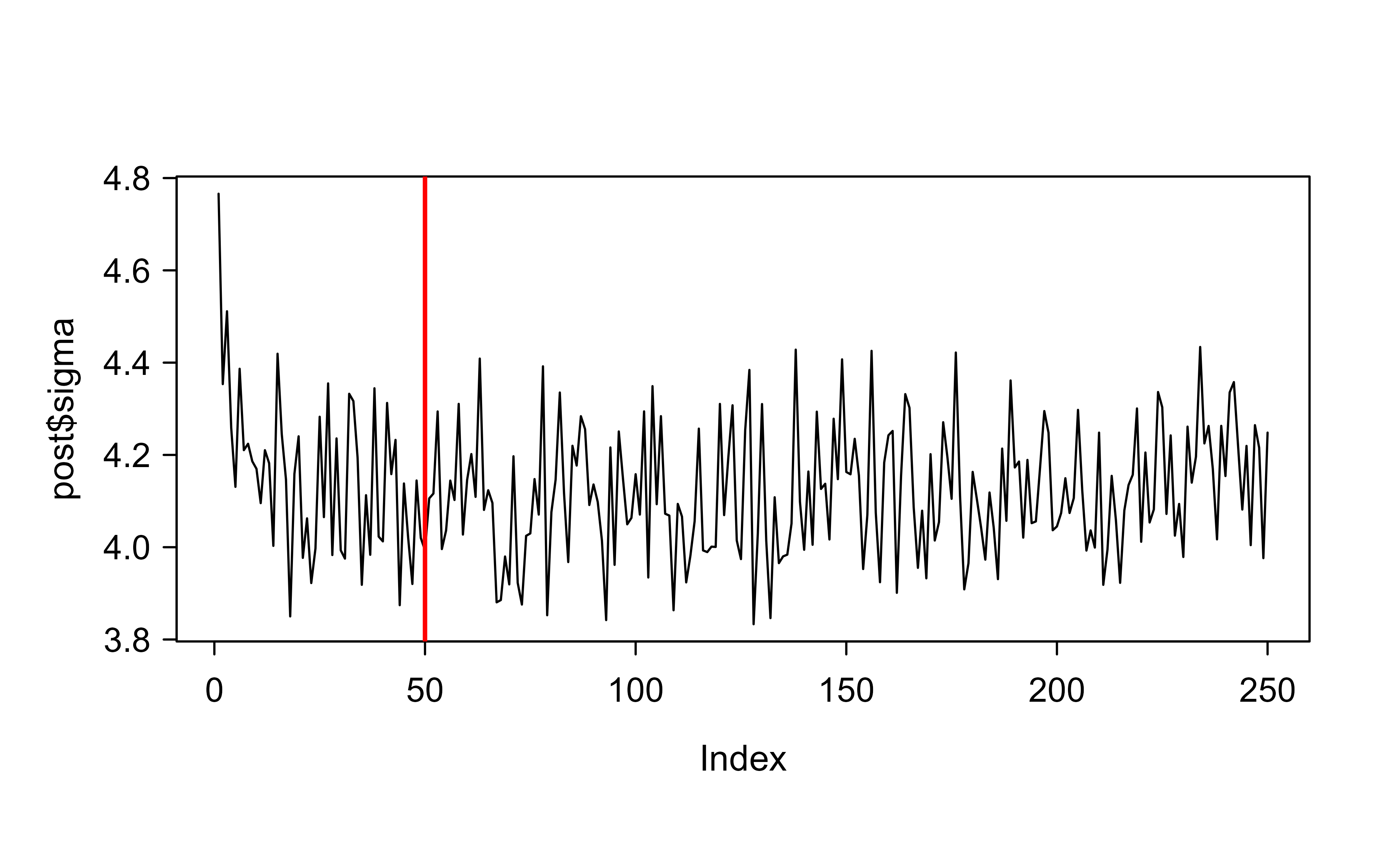
Because BART is an MCMC method, we should never trust the output until we have checked that the chain actually converged. A standard diagnostic is to plot the sampled error standard deviation sigma across iterations: if the chain has settled, the trace should stop drifting and fluctuate around a stable level. Figure 14.2 shows this trace, where the red line marks the end of the burn-in period.
Show code
plot(post$sigma, type ="l")abline(v =burn, lwd =2, col ="red")# good convergence
Figure 14.2: Trace of the sampled error standard deviation sigma across MCMC iterations. The vertical red line marks the end of the burn-in period; the trace flattens and fluctuates around a stable level, indicating good convergence.
The trace flattens out quickly and stays level after burn-in, which indicates good convergence. If instead you saw a slow drift or a trend that never stabilized, the remedy would be to increase the burn-in (and possibly the total number of draws) and refit.
Warning
Skipping this convergence check is the most common BART mistake. Point predictions can look reasonable even when the chain has not mixed, but the uncertainty intervals you report will be wrong.
14.4.2 Comparing predictions with linear regression
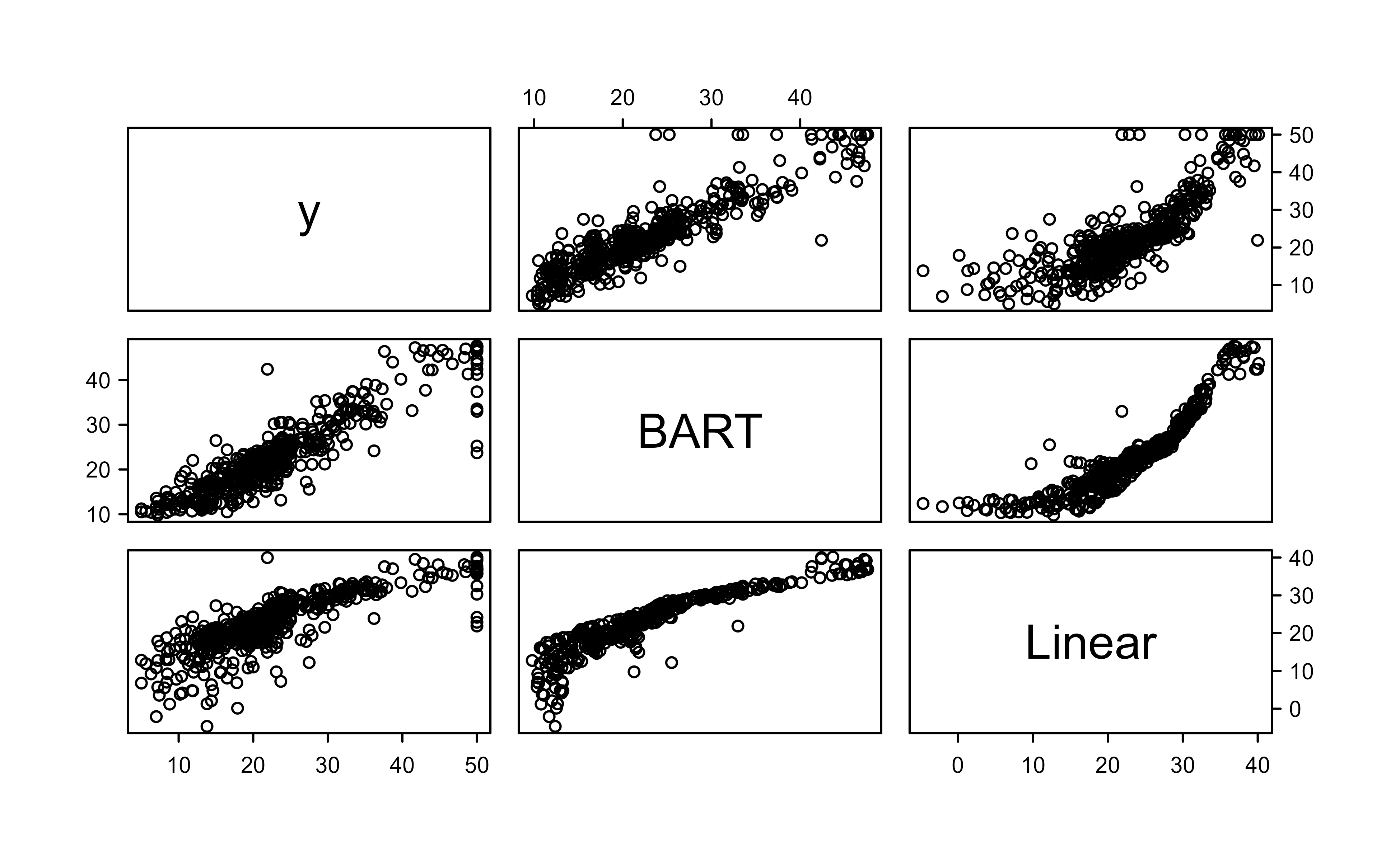
To put BART’s fitted values in context, we compare them against ordinary linear regression on the same two predictors. We line up the observed y, the BART fitted means, and the linear model fitted values, then look at their correlations and the pairwise scatterplots in Figure 14.3.
Show code
lmf<-lm(y~., data.frame(x, y))fitmat<-cbind(y, post$yhat.train.mean, lmf$fitted.values)colnames(fitmat)<-c("y", "BART", "Linear")cor(fitmat)#> y BART Linear#> y 1.0000000 0.9051200 0.7991005#> BART 0.9051200 1.0000000 0.8978003#> Linear 0.7991005 0.8978003 1.0000000pairs(fitmat)
Figure 14.3: Pairwise scatterplots of the observed response, BART fitted means, and linear-regression fitted values. The BART fitted values track the observed response more closely than the linear fit.
The correlation matrix and the scatterplots tell the story: BART’s fitted values track the observed response more closely than the linear fit, which is what we expect when the true relationship is nonlinear (the rooms and lower-status effects both bend rather than running in straight lines).
14.4.3 From point predictions to uncertainty
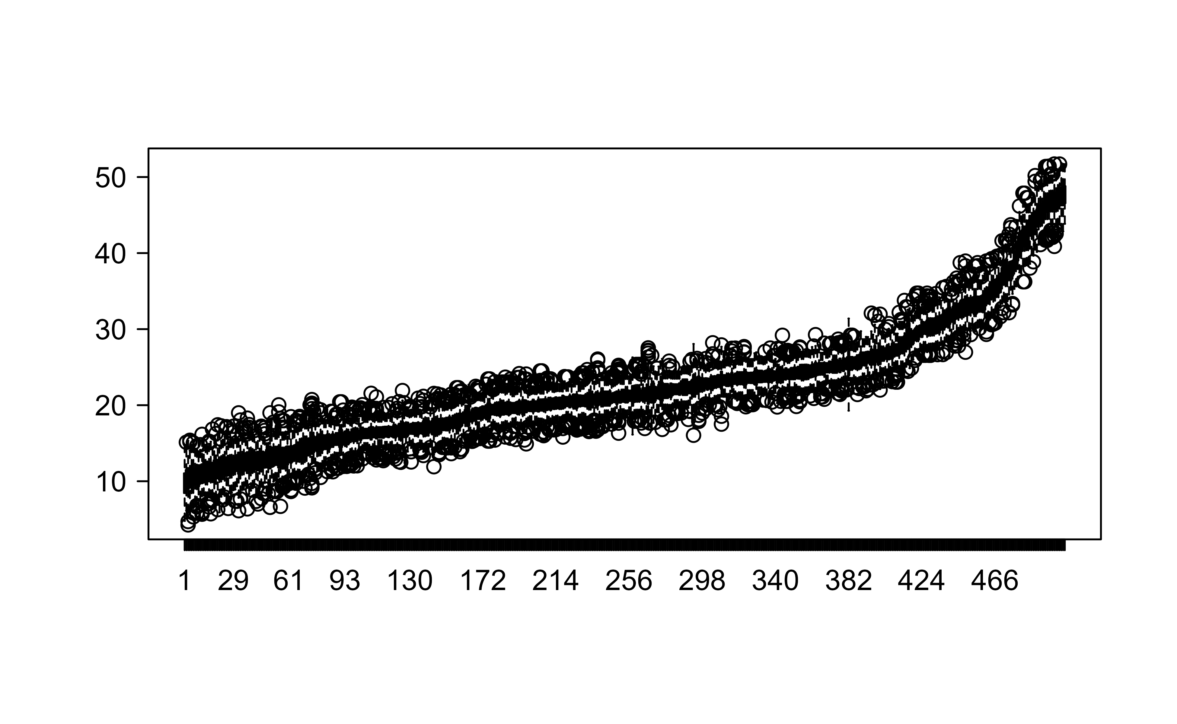
One of BART’s selling points is that every prediction comes with a posterior distribution, not just a single number. Figure 14.4 shows, for each training observation (sorted by its fitted mean), the spread of predictions across the retained posterior draws. Wider boxes mean more uncertainty about that observation’s prediction.
Show code
i<-order(post$yhat.train.mean)boxplot(post$yhat.train[, i])n<-length(y)set.seed(14)i<-sample(1:n, floor(0.75*n))x.train<-x[i, ]; y.train=y[i]x.test<-x[-i, ]; y.test=y[-i]cat("training sample size = ", length(y.train), "\n")#> training sample size = 379cat("testing sample size = ", length(y.test), "\n")#> testing sample size = 127set.seed(99)post1<-wbart(x.train, y.train, x.test)#> *****Into main of wbart#> *****Data:#> data:n,p,np: 379, 2, 127#> y1,yn: 14.101319, -7.098681#> x1,x[n*p]: 7.206000, 12.120000#> xp1,xp[np*p]: 6.421000, 23.970000#> *****Number of Trees: 200#> *****Number of Cut Points: 100 ... 100#> *****burn and ndpost: 100, 1000#> *****Prior:beta,alpha,tau,nu,lambda: 2.000000,0.950000,0.795495,3.000000,6.258099#> *****sigma: 5.668084#> *****w (weights): 1.000000 ... 1.000000#> *****Dirichlet:sparse,theta,omega,a,b,rho,augment: 0,0,1,0.5,1,2,0#> *****nkeeptrain,nkeeptest,nkeeptestme,nkeeptreedraws: 1000,1000,1000,1000#> *****printevery: 100#> *****skiptr,skipte,skipteme,skiptreedraws: 1,1,1,1#> #> MCMC#> done 0 (out of 1100)#> done 100 (out of 1100)#> done 200 (out of 1100)#> done 300 (out of 1100)#> done 400 (out of 1100)#> done 500 (out of 1100)#> done 600 (out of 1100)#> done 700 (out of 1100)#> done 800 (out of 1100)#> done 900 (out of 1100)#> done 1000 (out of 1100)#> time: 6s#> check counts#> trcnt,tecnt,temecnt,treedrawscnt: 1000,1000,1000,1000length(post1$yhat.test.mean)#> [1] 127
Figure 14.4: Boxplots of the posterior predictive draws for each training observation, sorted by fitted mean. Wider boxes indicate greater predictive uncertainty for that observation.
In the same chunk we also create a proper 75/25 train/test split and refit, producing test-set predictions in post1. The length check confirms we get one predicted mean per test observation.
14.4.4 Thinning to save time and memory
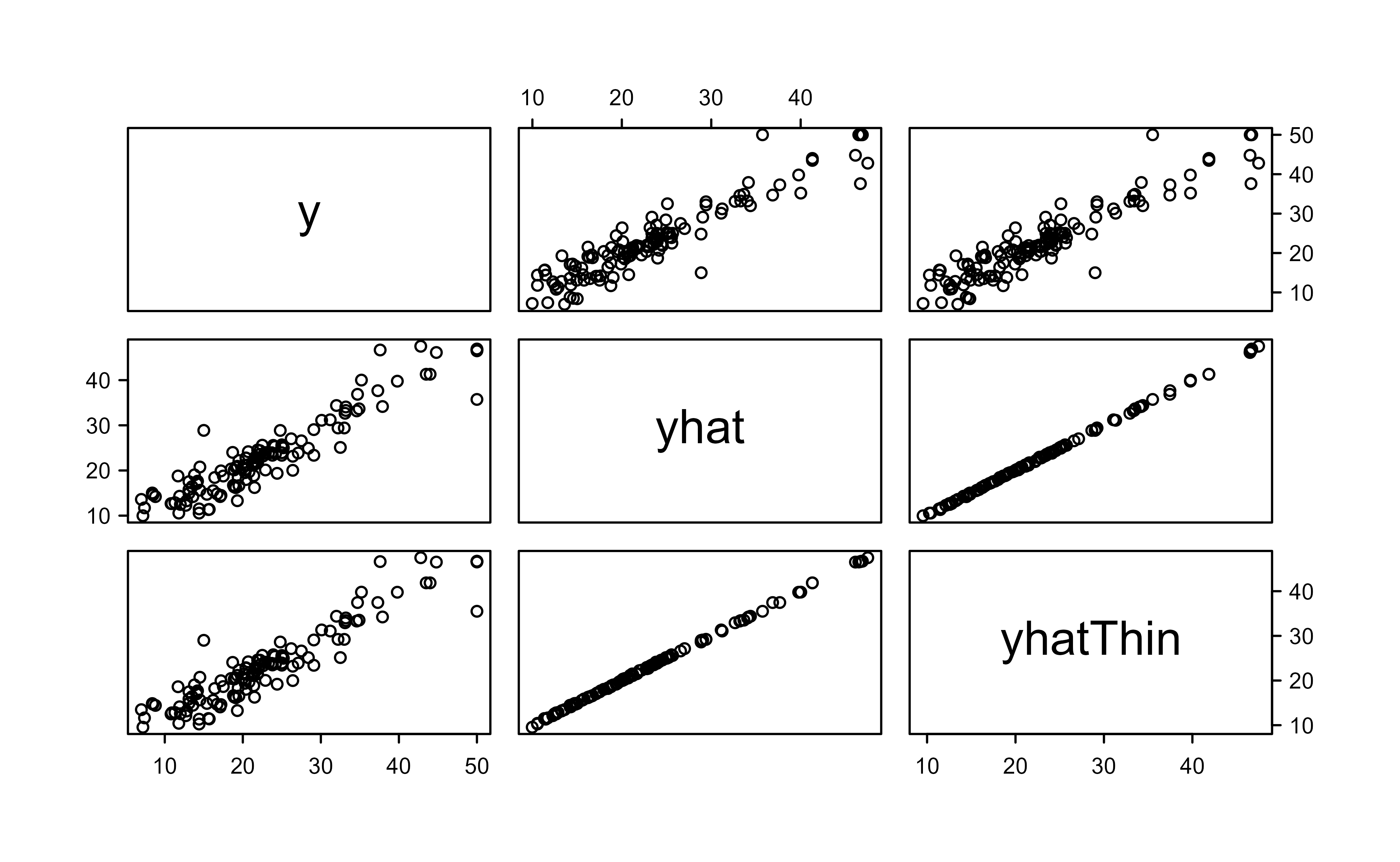
Long MCMC runs can produce huge output objects, and consecutive draws are correlated anyway, so we often thin the chain: run many iterations but keep only a subset. Thinning trades a little statistical efficiency for large savings in memory and storage. Below we run a long chain (1000 burn-in, 10000 draws) but keep only 200 tree draws, then predict on the test set and compare against the earlier, unthinned predictions in Figure 14.5.4
Show code
set.seed(4)post3<-wbart(x.train,y.train, nskip =1000, ndpost =10000, nkeeptrain =0, nkeeptest =0, nkeeptestmean =0, nkeeptreedraws =200)#> *****Into main of wbart#> *****Data:#> data:n,p,np: 379, 2, 0#> y1,yn: 14.101319, -7.098681#> x1,x[n*p]: 7.206000, 12.120000#> *****Number of Trees: 200#> *****Number of Cut Points: 100 ... 100#> *****burn and ndpost: 1000, 10000#> *****Prior:beta,alpha,tau,nu,lambda: 2.000000,0.950000,0.795495,3.000000,6.258099#> *****sigma: 5.668084#> *****w (weights): 1.000000 ... 1.000000#> *****Dirichlet:sparse,theta,omega,a,b,rho,augment: 0,0,1,0.5,1,2,0#> *****nkeeptrain,nkeeptest,nkeeptestme,nkeeptreedraws: 0,0,0,200#> *****printevery: 100#> *****skiptr,skipte,skipteme,skiptreedraws: 10001,10001,10001,50#> #> MCMC#> done 0 (out of 11000)#> done 100 (out of 11000)#> done 200 (out of 11000)#> done 300 (out of 11000)#> done 400 (out of 11000)#> done 500 (out of 11000)#> done 600 (out of 11000)#> done 700 (out of 11000)#> done 800 (out of 11000)#> done 900 (out of 11000)#> done 1000 (out of 11000)#> done 1100 (out of 11000)#> done 1200 (out of 11000)#> done 1300 (out of 11000)#> done 1400 (out of 11000)#> done 1500 (out of 11000)#> done 1600 (out of 11000)#> done 1700 (out of 11000)#> done 1800 (out of 11000)#> done 1900 (out of 11000)#> done 2000 (out of 11000)#> done 2100 (out of 11000)#> done 2200 (out of 11000)#> done 2300 (out of 11000)#> done 2400 (out of 11000)#> done 2500 (out of 11000)#> done 2600 (out of 11000)#> done 2700 (out of 11000)#> done 2800 (out of 11000)#> done 2900 (out of 11000)#> done 3000 (out of 11000)#> done 3100 (out of 11000)#> done 3200 (out of 11000)#> done 3300 (out of 11000)#> done 3400 (out of 11000)#> done 3500 (out of 11000)#> done 3600 (out of 11000)#> done 3700 (out of 11000)#> done 3800 (out of 11000)#> done 3900 (out of 11000)#> done 4000 (out of 11000)#> done 4100 (out of 11000)#> done 4200 (out of 11000)#> done 4300 (out of 11000)#> done 4400 (out of 11000)#> done 4500 (out of 11000)#> done 4600 (out of 11000)#> done 4700 (out of 11000)#> done 4800 (out of 11000)#> done 4900 (out of 11000)#> done 5000 (out of 11000)#> done 5100 (out of 11000)#> done 5200 (out of 11000)#> done 5300 (out of 11000)#> done 5400 (out of 11000)#> done 5500 (out of 11000)#> done 5600 (out of 11000)#> done 5700 (out of 11000)#> done 5800 (out of 11000)#> done 5900 (out of 11000)#> done 6000 (out of 11000)#> done 6100 (out of 11000)#> done 6200 (out of 11000)#> done 6300 (out of 11000)#> done 6400 (out of 11000)#> done 6500 (out of 11000)#> done 6600 (out of 11000)#> done 6700 (out of 11000)#> done 6800 (out of 11000)#> done 6900 (out of 11000)#> done 7000 (out of 11000)#> done 7100 (out of 11000)#> done 7200 (out of 11000)#> done 7300 (out of 11000)#> done 7400 (out of 11000)#> done 7500 (out of 11000)#> done 7600 (out of 11000)#> done 7700 (out of 11000)#> done 7800 (out of 11000)#> done 7900 (out of 11000)#> done 8000 (out of 11000)#> done 8100 (out of 11000)#> done 8200 (out of 11000)#> done 8300 (out of 11000)#> done 8400 (out of 11000)#> done 8500 (out of 11000)#> done 8600 (out of 11000)#> done 8700 (out of 11000)#> done 8800 (out of 11000)#> done 8900 (out of 11000)#> done 9000 (out of 11000)#> done 9100 (out of 11000)#> done 9200 (out of 11000)#> done 9300 (out of 11000)#> done 9400 (out of 11000)#> done 9500 (out of 11000)#> done 9600 (out of 11000)#> done 9700 (out of 11000)#> done 9800 (out of 11000)#> done 9900 (out of 11000)#> done 10000 (out of 11000)#> done 10100 (out of 11000)#> done 10200 (out of 11000)#> done 10300 (out of 11000)#> done 10400 (out of 11000)#> done 10500 (out of 11000)#> done 10600 (out of 11000)#> done 10700 (out of 11000)#> done 10800 (out of 11000)#> done 10900 (out of 11000)#> time: 38s#> check counts#> trcnt,tecnt,temecnt,treedrawscnt: 0,0,0,200yhatthin<-predict(post3, x.test)#> *****In main of C++ for bart prediction#> tc (threadcount): 1#> number of bart draws: 200#> number of trees in bart sum: 200#> number of x columns: 2#> from x,np,p: 2, 127#> ***using serial codefmat<-cbind(y.test, post1$yhat.test.mean, apply(yhatthin, 2, mean))colnames(fmat)<-c("y", "yhat", "yhatThin")pairs(fmat)
Figure 14.5: Pairwise scatterplots of the observed test response, the full unthinned predictions (yhat), and the thinned predictions (yhatThin). The thinned predictions line up closely with the full predictions.
The scatterplots show that the thinned predictions (yhatThin) line up closely with the full predictions (yhat), confirming that thinning here costs us almost nothing in accuracy while keeping the stored model small.
14.4.5 Variable importance via partial dependence
Finally, we look at variable importance in a way that shows not just whether a variable matters but how it shapes the prediction. Friedman’s partial dependence function answers the question: if we sweep one predictor across its range while averaging over the distribution of all the other predictors, how does the predicted response move?
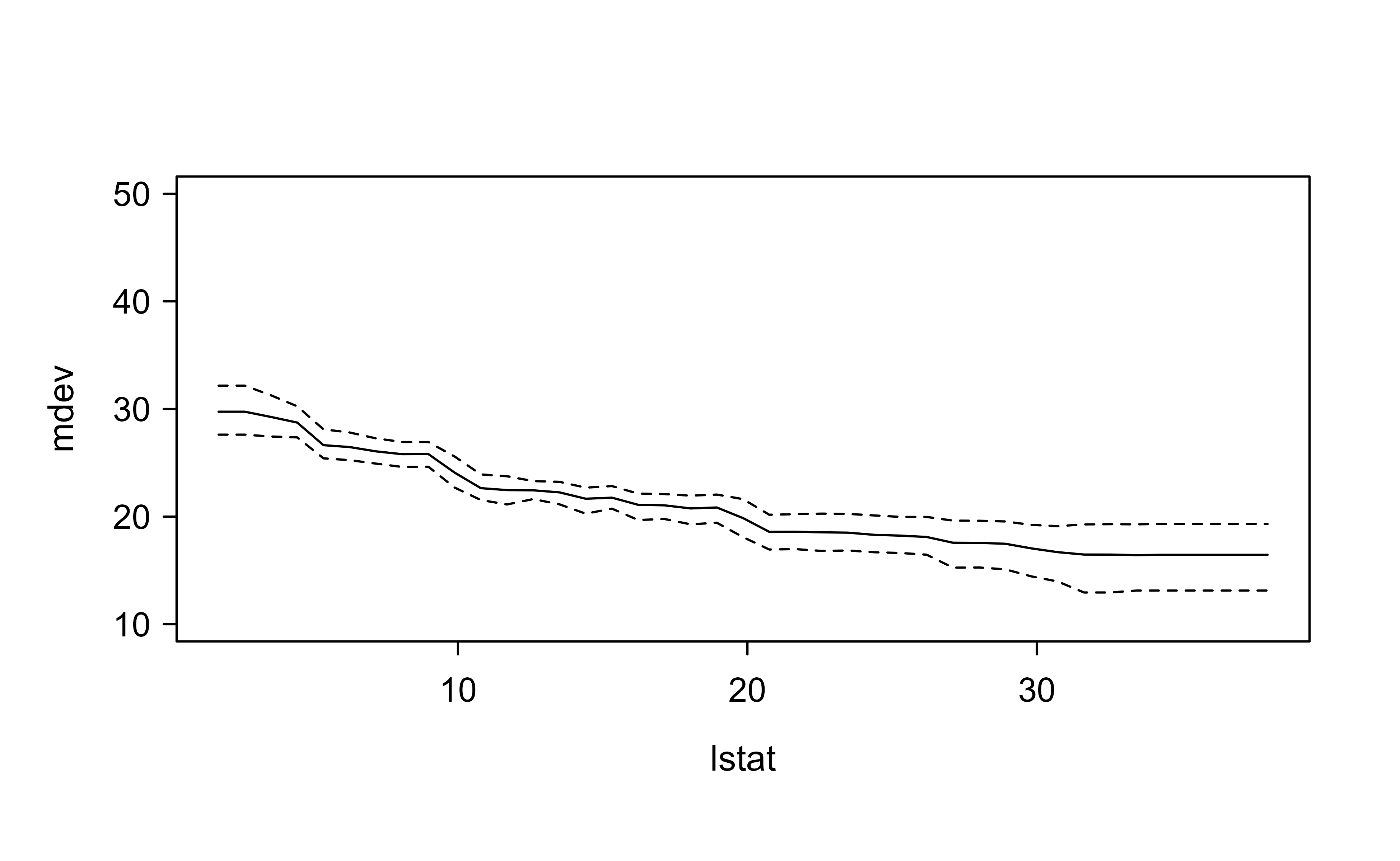
The procedure builds a grid of values for lstat (the 13th column), replaces that column with each grid value while holding the other columns at their observed combinations, predicts, and averages. In Figure 14.6, the solid line is the average partial-dependence curve and the dashed lines are pointwise 2.5% and 97.5% posterior quantiles, giving an uncertainty band around the effect.
Show code
x.train<-as.matrix(MASS::Boston[i,-14])set.seed(12)post4<-wbart(x.train, y.train)#> *****Into main of wbart#> *****Data:#> data:n,p,np: 379, 13, 0#> y1,yn: 14.101319, -7.098681#> x1,x[n*p]: 0.550070, 12.120000#> *****Number of Trees: 200#> *****Number of Cut Points: 100 ... 100#> *****burn and ndpost: 100, 1000#> *****Prior:beta,alpha,tau,nu,lambda: 2.000000,0.950000,0.795495,3.000000,4.636409#> *****sigma: 4.878720#> *****w (weights): 1.000000 ... 1.000000#> *****Dirichlet:sparse,theta,omega,a,b,rho,augment: 0,0,1,0.5,1,13,0#> *****nkeeptrain,nkeeptest,nkeeptestme,nkeeptreedraws: 1000,1000,1000,1000#> *****printevery: 100#> *****skiptr,skipte,skipteme,skiptreedraws: 1,1,1,1#> #> MCMC#> done 0 (out of 1100)#> done 100 (out of 1100)#> done 200 (out of 1100)#> done 300 (out of 1100)#> done 400 (out of 1100)#> done 500 (out of 1100)#> done 600 (out of 1100)#> done 700 (out of 1100)#> done 800 (out of 1100)#> done 900 (out of 1100)#> done 1000 (out of 1100)#> time: 6s#> check counts#> trcnt,tecnt,temecnt,treedrawscnt: 1000,0,0,1000H<-length(y.train)L<-41x<-seq(min(x.train[, 13]), max(x.train[, 13]), length.out =L)x.test<-cbind(x.train[,-13], x[1])for(jin2:L)x.test<-rbind(x.test, cbind(x.train[,-13], x[j]))pred<-predict(post4, x.test)#> *****In main of C++ for bart prediction#> tc (threadcount): 1#> number of bart draws: 1000#> number of trees in bart sum: 200#> number of x columns: 13#> from x,np,p: 13, 15539#> ***using serial codepartial<-matrix(nrow =1000, ncol =L)for(jin1:L){h<-(j-1)*H+1:Hpartial[, j]<-apply(pred[, h], 1, mean)}plot(x,apply(partial, 2, mean), type ="l", ylim =c(10, 50), xlab ="lstat", ylab ="mdev")lines(x, apply(partial, 2, quantile, probs =0.025), lty =2)lines(x, apply(partial, 2, quantile, probs =0.975), lty =2)
Figure 14.6: Partial dependence of predicted median home value on the lower-status percentage (lstat). The solid line is the average partial-dependence curve and the dashed lines are pointwise 2.5% and 97.5% posterior quantiles.
The curve slopes clearly downward: as the lower-status percentage increases, predicted median home value falls, and the decline is steeper at low values of lstat than at high ones (a nonlinear effect a linear model would miss). The dashed band reminds us that this estimated effect is itself uncertain, which is precisely the kind of honest summary BART was built to provide.
Tip
Partial dependence plots are model-agnostic. You met the same idea in the chapter on interpretable machine learning (Chapter 35), and you can apply it to random forests, boosting, or BART alike. What is special here is that BART hands you a credible band for free, straight from its posterior draws.
14.5 Summary
BART models a response as a sum of many small trees and fits them with an MCMC sampler that repeatedly perturbs each tree toward the partial residual left by the others. Keeping trees small and updates gentle controls overfitting, while the Bayesian machinery delivers full posterior distributions, so every prediction, variable-importance summary, and partial-dependence curve comes with honest uncertainty. With sensible defaults (many trees, a long chain, a moderate burn-in), it works well with little tuning, which is why it is a reliable first choice for flexible regression and classification.
Chipman, Hugh A., Edward I. George, and Robert E. McCulloch. 2010. “BART: Bayesian Additive Regression Trees.”The Annals of Applied Statistics 4 (1): 266–98. https://doi.org/10.1214/09-AOAS285.
James, Gareth, Daniela Witten, Trevor Hastie, and Robert Tibshirani. 2013. “Statistical Learning.” In, 15–57. Springer New York. https://doi.org/10.1007/978-1-4614-7138-7_2.
Ročková, Veronika, and Stéphanie van der Pas. 2020. “Posterior Concentration for Bayesian Regression Trees and Forests.”The Annals of Statistics 48 (4): 2108–31. https://doi.org/10.1214/19-AOS1879.
Sparapani, Rodney, Charles Spanbauer, and Robert McCulloch. 2021. “Nonparametric Machine Learning and Efficient Computation with Bayesian Additive Regression Trees: The BART R Package.”Journal of Statistical Software 97 (1). https://doi.org/10.18637/jss.v097.i01.
The difference is that boosting fits each new tree to the residuals once, in a forward, greedy pass, while BART repeatedly revisits and revises every tree using a Markov chain Monte Carlo sampler. This revisiting is what produces a posterior distribution instead of a single fitted model.↩︎
Mechanically, this is a Metropolis-Hastings step: a candidate change to the tree is proposed at random, and it is accepted or rejected with a probability that depends on how much it improves the fit and on the prior. Over many iterations the trees are effectively samples from a posterior distribution.↩︎
nskip is the burn-in count \(L\) and ndpost is the number of retained posterior draws. They correspond directly to the \(L\) and \(B - L\) in the algorithm above.↩︎
The nkeep* arguments control which parts of the output are stored. Setting nkeeptrain, nkeeptest, and nkeeptestmean to 0 tells wbart not to keep those potentially large matrices, while nkeeptreedraws = 200 keeps 200 tree ensembles so we can still predict later with predict.↩︎
Source Code
# Bayesian Additive Regression Trees {#sec-bart}```{r}#| include: falsesource("_common.R")```Imagine you want to predict the price of a house from its features (number of rooms, neighborhood income, distance to work, and so on). A single regression tree (@sec-regression-trees) is easy to read but usually too crude. A forest of many trees (@sec-random-forest) predicts well but gives you a single point estimate with no honest sense of how uncertain that estimate is. Bayesian Additive Regression Trees, or BART [@sparapani2021], try to give you the best of both: the flexibility of a sum of many small trees, plus a full probability distribution over the prediction so you can attach uncertainty to every number you report.This chapter introduces BART from intuition first, then states the algorithm precisely, and finally walks through worked examples in R using the `BART` package. By the end you should understand why BART is often called a "good out-of-the-box" method, how its three main settings (number of trees, number of iterations, and burn-in) work, and how to read its output, including convergence checks, variable importance, and partial dependence plots.::: {.callout-tip title="When to use this"}BART is a strong default when you want flexible, nonlinear regression or classification with little tuning, and you also want uncertainty intervals around predictions. It pairs naturally with the tree-based and ensemble ideas you have already seen.:::BART sits in the same family as the methods in the chapters on bagging (@sec-bagging), random forests (@sec-random-forest), and boosting (@sec-boosting), and it borrows one key idea from each. As in bagging and random forests, every tree is built using randomness rather than a single deterministic greedy search. As in boosting, every tree tries to capture the part of the signal that the rest of the model has not yet explained.^[The difference is that boosting fits each new tree to the residuals once, in a forward, greedy pass, while BART repeatedly *revisits and revises* every tree using a Markov chain Monte Carlo sampler. This revisiting is what produces a posterior distribution instead of a single fitted model.]## The model: a sum of treesThe core idea is simple to state. Instead of one big tree, BART uses a *sum* of many small trees, and each tree contributes a small piece of the final prediction.Let $K$ be the number of regression trees, and let $B$ be the number of MCMC iterations for which the BART algorithm will be run. Let $\hat{f}_k^b(x)$ represent the prediction at $x$ for the $k$-th regression tree used in the $b$-th iteration. The prediction from a single iteration is the sum of all $K$ trees in that iteration:$$\hat{f}^b(x) = \sum_{k=1}^K \hat{f}_k^b(x), b = 1, \dots, B$$::: {.callout-important title="Key idea"}No single tree has to be good on its own. Each tree is deliberately kept small (a "weak learner"), and the prediction comes from adding many of them together. Keeping each tree small is the main guard against overfitting.:::### The probabilistic model and likelihoodThe algorithmic description above hides a fully specified Bayesian model, which we now write out precisely because every step of the sampler (the random perturbations, the "favoring" of good fits, even the burn-in) is a consequence of it. Following @chipman2010, the original BART paper, we write a single tree as a pair $(T_k, M_k)$, where $T_k$ encodes the tree topology, that is, the internal splitting rules (each a variable index and a split value) and the leaf structure, and $M_k = \{\mu_{k1}, \dots, \mu_{kb_k}\}$ collects the scalar parameters stored in its $b_k$ terminal nodes. Writing $g(x; T_k, M_k)$ for the function that drops $x$ down tree $T_k$ and returns the leaf value, the model is the sum of trees plus Gaussian noise,$$y_i = \sum_{k=1}^K g(x_i; T_k, M_k) + \varepsilon_i, \qquad \varepsilon_i \stackrel{iid}{\sim} N(0, \sigma^2).$$ {#eq-BART-model}The unknowns are the $K$ trees $\{(T_k, M_k)\}_{k=1}^K$ and the error variance $\sigma^2$. The likelihood implied by @eq-BART-model is$$p(y \mid \{T_k, M_k\}, \sigma^2) = \prod_{i=1}^n N\!\left(y_i;\ \textstyle\sum_{k=1}^K g(x_i; T_k, M_k),\ \sigma^2\right).$$ {#eq-BART-lik}::: {.callout-note}Before fitting, the continuous response is centered and scaled (the `BART` package rescales $y$ to the interval $[-0.5, 0.5]$). This is not cosmetic: it is what lets the same default prior hyperparameters work across data sets with wildly different units, which is a large part of why BART is "out of the box.":::### The prior: regularization made explicitWhat stops a sum of $K = 200$ trees from interpolating the data is the prior, not the likelihood. BART places independent priors on the trees and on the variance, and assumes the trees are mutually independent and independent of $\sigma$:$$p\big(\{T_k, M_k\}, \sigma^2\big) = \left[\prod_{k=1}^K p(M_k \mid T_k)\, p(T_k)\right] p(\sigma^2),\qquad p(M_k \mid T_k) = \prod_{j=1}^{b_k} p(\mu_{kj} \mid T_k).$$ {#eq-BART-prior}There are three pieces, each doing a specific regularizing job.**Tree-shape prior $p(T_k)$.** A node at depth $d$ (root is $d = 0$) is made internal, that is, split rather than left as a leaf, with probability$$p_{\text{split}}(d) = \alpha\, (1 + d)^{-\beta}, \qquad \alpha \in (0,1),\ \beta \ge 0.$$ {#eq-BART-split}The factor $(1+d)^{-\beta}$ makes deeper splits polynomially less likely, so the prior concentrates on shallow "stumpy" trees. The `BART` defaults are $\alpha = 0.95$ and $\beta = 2$, under which the prior probability of a tree of depth $0, 1, 2, 3$ being a single node, then splitting once, twice, and so on, puts the overwhelming mass on trees with one or two levels: with $\beta = 2$ the split probabilities are $0.95$ at the root, $0.95/4 \approx 0.24$ at depth 1, $0.95/9 \approx 0.11$ at depth 2. Given that a node splits, the splitting variable is drawn uniformly over available predictors and the split point uniformly over its available values.**Leaf-value prior $p(\mu_{kj} \mid T_k)$.** Each leaf parameter gets a conjugate Gaussian prior centered at zero,$$\mu_{kj} \mid T_k \sim N(0,\ \sigma_\mu^2).$$ {#eq-BART-mu-prior}Centering at zero is sensible because the response has been centered, and the $K$ trees share the signal additively, so each leaf should contribute only a small piece. The variance $\sigma_\mu^2$ is set so that the prior on the sum, $E[Y \mid x] = \sum_k g(x; T_k, M_k)$, which by independence has variance $K \sigma_\mu^2$, places most of its mass on the observed range of $y$. Concretely, @chipman2010 choose $\sigma_\mu = 0.5/(c\sqrt{K})$ on the rescaled response, where $c$ (default $c = 2$) is the number of prior standard deviations of the centered response that should fit in the half-range $0.5$. The crucial consequence is the $1/\sqrt{K}$ shrinkage: adding more trees automatically shrinks each leaf, so $K$ controls model complexity gently rather than catastrophically.**Error-variance prior $p(\sigma^2)$.** A conjugate inverse-gamma prior is used, written as a scaled inverse chi-squared,$$\sigma^2 \sim \frac{\nu\,\lambda}{\chi^2_\nu}, \qquad \text{equivalently}\qquad \sigma^2 \sim \text{Inv-Gamma}\!\left(\tfrac{\nu}{2},\ \tfrac{\nu\lambda}{2}\right).$$ {#eq-BART-sigma-prior}The degrees of freedom $\nu$ (default $3$) controls the tail, and $\lambda$ is calibrated from the data so that a chosen prior quantile $q$ (default $0.90$) of $\sigma$ falls at a rough overestimate of the noise level, typically the residual standard deviation $\hat\sigma$ from a least-squares fit of $y$ on $X$. This anchors the variance prior to the data's scale while keeping it weakly informative.### Starting pointWe need a place to begin the chain. In the first iteration, all trees are initialized to have a single root node with $\hat{f}_k^1(x) = (1/nK)\sum_{i=1}^n y_i$, which is the mean of the response values divided by the total number of trees. Splitting the overall mean equally across the $K$ trees means that when we add the trees back up, we recover exactly the mean response:$$\hat{f}^1(x) = \sum_{k=1}^K \hat{f}_k^1 (x) = \frac{1}{n} \sum_{i=1}^n y_i \text{ (mean response)}$$::: {.callout-tip title="Intuition"}BART starts from the simplest possible prediction, "guess the average for everyone," and then lets the trees gradually carve out structure from there.:::### Updating one tree at a time using partial residualsIn each later iteration, BART updates each of the $K$ trees, one at a time. The trick that makes this work is the *partial residual*: when we are about to update tree $k$, we temporarily remove its contribution and ask how far off the *rest* of the model is. Whatever the other trees fail to explain is exactly what tree $k$ should try to capture.Concretely, in the $b$-th iteration, to update the $k$-th tree, we subtract from each response value the predictions from all but the $k$-th tree to obtain a partial residual:$$r_i = y_i - \sum_{k'<k} \hat{f}_{k'}^b (x_i) - \sum_{k'>k} \hat{f}_{k'}^{b-1}(x_i), i = 1, \dots, n$$Notice the bookkeeping in the two sums: trees with index $k' < k$ have already been updated in the current iteration $b$, so we use their fresh values, while trees with $k' > k$ have not been touched yet this round, so we use their values from the previous iteration $b-1$.Here is the step that makes BART Bayesian rather than just another boosting scheme. Instead of fitting a brand new tree to this partial residual, BART randomly chooses a perturbation to the tree from the previous iteration ($\hat{f}_k^{b-1}$) out of a set of possible perturbations (this is where MCMC comes in), favoring ones that improve the fit to the partial residual.^[Mechanically, this is a Metropolis-Hastings step: a candidate change to the tree is proposed at random, and it is accepted or rejected with a probability that depends on how much it improves the fit and on the prior. Over many iterations the trees are effectively samples from a posterior distribution.] There are two components to this perturbation, which we apply together:- change the structure of the tree by adding or pruning branches, and- change the prediction value stored in each terminal (leaf) node of the tree.::: {.callout-note}Because we *perturb* the existing tree rather than regrowing it from scratch, no single update can move the model very far. This deliberate timidity is what keeps BART from chasing noise.:::### Deriving the Bayesian backfitting updateThe phrase "favoring perturbations that improve the fit" is, made precise, a Gibbs sampler that draws each unknown from its full conditional given everything else, a scheme @chipman2010 call Bayesian backfitting. We now derive each conditional. Condition throughout on $\sigma^2$ and on all trees other than the $k$-th, and let $r = (r_1, \dots, r_n)$ be the partial residual defined above. By construction $r_i = g(x_i; T_k, M_k) + \varepsilon_i$, so the $k$-th tree sees a clean single-tree regression problem with response $r$. The full conditional for $(T_k, M_k)$ depends on the others only through $r$:$$p(T_k, M_k \mid r, \sigma^2) \propto p(r \mid T_k, M_k, \sigma^2)\, p(M_k \mid T_k)\, p(T_k).$$ {#eq-BART-fullcond}BART draws this in two steps: first $T_k \mid r, \sigma^2$ with $M_k$ integrated out, then $M_k \mid T_k, r, \sigma^2$.**Step 1: integrate out the leaves to get the marginal likelihood.** Because the Gaussian leaf prior @eq-BART-mu-prior is conjugate to the Gaussian likelihood, we can integrate $M_k$ out in closed form, which is what makes the tree move feasible. The tree partitions the $n$ residuals into the leaves; let leaf $j$ contain the index set with $n_j$ residuals, sum $S_j = \sum_{i \in \text{leaf } j} r_i$, and let the leaf parameters be independent across leaves. For a single leaf with $n_j$ observations $r_i \sim N(\mu, \sigma^2)$ and prior $\mu \sim N(0, \sigma_\mu^2)$, completing the square in $\mu$ gives the marginal$$p(\{r_i\}_{i \in j} \mid T_k, \sigma^2) = \int \prod_{i \in j} N(r_i; \mu, \sigma^2)\, N(\mu; 0, \sigma_\mu^2)\, d\mu= \frac{(2\pi\sigma^2)^{-n_j/2}}{\sqrt{1 + n_j \sigma_\mu^2/\sigma^2}}\,\exp\!\left\{-\frac{1}{2\sigma^2}\sum_{i \in j} r_i^2 + \frac{\sigma_\mu^2\, S_j^2}{2\sigma^2(\sigma^2 + n_j \sigma_\mu^2)}\right\}.$$ {#eq-BART-marglik}The full tree marginal likelihood is the product of @eq-BART-marglik over leaves $j = 1, \dots, b_k$. This scalar is the quantity that "scores" a candidate tree.**Step 2: the leaf posterior.** Given the tree, the leaves are conditionally independent and each is a standard conjugate normal-normal update. For leaf $j$,$$\mu_{kj} \mid T_k, r, \sigma^2 \sim N\!\left(\frac{S_j/\sigma^2}{\,n_j/\sigma^2 + 1/\sigma_\mu^2\,},\ \ \frac{1}{\,n_j/\sigma^2 + 1/\sigma_\mu^2\,}\right).$$ {#eq-BART-mu-post}The posterior mean is a precision-weighted average of the leaf's residual mean $S_j/n_j$ and the prior mean $0$, so leaves with few observations are shrunk hard toward zero. This is the exact mechanism behind "each tree contributes a small piece."We can confirm @eq-BART-mu-post numerically with a tiny simulation: draw residuals in one leaf, then check that the analytic posterior mean and variance match a brute-force Monte Carlo evaluation of the unnormalized posterior $\prod_i N(r_i;\mu,\sigma^2)\,N(\mu;0,\sigma_\mu^2)$.```{r}set.seed(1)nj <-8; sigma2 <-1.5; sigma_mu2 <-0.4r <-rnorm(nj, mean =1.2, sd =sqrt(sigma2)) # residuals in one leafSj <-sum(r)# analytic posterior from eq-BART.qmd-mu-postpost_var <-1/ (nj / sigma2 +1/ sigma_mu2)post_mean <- post_var * (Sj / sigma2)# brute-force normalization over a fine grid of mumu <-seq(-3, 3, length.out =20001)logpost <-sapply(mu, function(m)sum(dnorm(r, m, sqrt(sigma2), log =TRUE)) +dnorm(m, 0, sqrt(sigma_mu2), log =TRUE))w <-exp(logpost -max(logpost)); w <- w /sum(w)num_mean <-sum(mu * w)num_var <-sum((mu - num_mean)^2* w)c(analytic_mean = post_mean, numeric_mean = num_mean,analytic_var = post_var, numeric_var = num_var)```The analytic and numerical values agree to several digits, confirming the conjugate update.**Step 3: the Metropolis-Hastings move on tree structure.** The tree topology $T_k$ has no conjugate form, so it is updated with a Metropolis-Hastings step using @eq-BART-marglik as the marginalized target. A move $T_k \to T_k^\star$ is proposed from a kernel $q(\cdot \mid \cdot)$ that picks among GROW (split a leaf into two), PRUNE (collapse two sibling leaves into one), CHANGE (alter a split rule), and SWAP (exchange rules of a parent and child). The proposal is accepted with probability$$A = \min\left\{1,\ \underbrace{\frac{q(T_k \mid T_k^\star)}{q(T_k^\star \mid T_k)}}_{\text{proposal ratio}}\cdot \underbrace{\frac{p(T_k^\star)}{p(T_k)}}_{\text{tree prior ratio}}\cdot \underbrace{\frac{p(r \mid T_k^\star, \sigma^2)}{p(r \mid T_k, \sigma^2)}}_{\text{marginal likelihood ratio}}\right\}.$$ {#eq-BART-mh}The middle factor is where the depth penalty $p_{\text{split}}(d)$ from @eq-BART-split enters: a GROW move that deepens the tree must overcome the prior's reluctance to split, which is precisely the regularization. Because the likelihood ratio uses the marginalized form, only the leaves touched by the move (the split or pruned node) actually change the score, so each MH evaluation is cheap, $O(n_j)$ in the affected leaves rather than $O(n)$.**Step 4: update $\sigma^2$.** After all $K$ trees are refreshed, form the full residual $e_i = y_i - \sum_k g(x_i; T_k, M_k)$. Conjugacy of @eq-BART-sigma-prior gives the inverse-gamma full conditional$$\sigma^2 \mid \cdot \ \sim\ \text{Inv-Gamma}\!\left(\frac{\nu + n}{2},\ \frac{\nu\lambda + \sum_{i=1}^n e_i^2}{2}\right),$$ {#eq-BART-sigma-post}which is the trace plotted in the convergence diagnostic later in this chapter. One full sweep over @eq-BART-mh, @eq-BART-mu-post, and @eq-BART-sigma-post is one MCMC iteration $b$.### Collecting the outputAfter running the chain, the output of BART is not one model but a whole collection of prediction models, one per iteration:$$\hat{f}^b(x) = \sum_{k =1}^K \hat{f}_k^b (x) , b = 1, \dots, B$$Early iterations are unreliable because the chain has not yet settled down, so we discard the first $L$ iterations as a burn-in period and average over the rest:$$\hat{f}(x) = \frac{1}{B - L} \sum_{b = L +1}^B \hat{f}^b (x)$$The payoff of the Bayesian framing appears here: because each retained iteration is a posterior sample, we are not limited to the average. We can use the spread of the posterior samples to get distributional estimates of the predictions, that is, credible intervals rather than just point predictions.::: {.callout-tip}When someone asks "how confident are you in this prediction?", BART has a direct answer: look at the variability of $\hat{f}^b(x)$ across the retained iterations.:::## The BART algorithmPutting the pieces together, the full procedure is summarized below, following [@james2013] Alg 8.3. The outer loop walks through MCMC iterations, the middle loop walks through the $K$ trees, and the inner loop computes the partial residual for each observation before perturbing the current tree.1. Let $\hat{f}_1^1(x) = \hat{f}_2^1(x) = \dots = \hat{f}_K^1(x) = \frac{1}{nK} \sum_{i=1}^n y_i$2. Compute $\hat{f}^1 (x) = \sum_{k=1}^K \hat{f}_k^1 (x) = \frac{1}{n}\sum_{i=1}^n y_i$3. For $b = 2, \dots, B$ 1. For $k = 1, \dots, K$ 1. For $i = 1, \dots , n$, compute the current partial residual ($r_i$) 2. Fit a new tree $\hat{f}_k^b(x)$ to $r_i$ by randomly perturbing the $k$-th tree from the previous iteration, $\hat{f}_k^{b-1}(x)$ (favor perturbations that improve the fit) 2. Compute $\hat{f}^b (x) = \sum_{k=1}^K \hat{f}^b_k (x)$4. Compute the mean after $L$ burn-in samples $\hat{f}(x) = \frac{1}{B - L} \sum_{b = L +1}^B \hat{f}^b (x)$A few remarks make the algorithm easier to reason about. Step 3.1.2 prevents overfitting because it limits how hard we fit the data in each iteration: a single perturbation can only nudge a tree a little. The individual trees are kept quite small on purpose; limiting tree size is another guard against overfitting, since very large trees would memorize the training data. And, as noted above, each time we randomly perturb a tree to fit the residuals we are effectively drawing a new tree from a posterior distribution.When we use BART, we have to specify three quantities:- the number of trees $K$,- the number of iterations $B$, and- the number of burn-in iterations $L$.In practice these are easy to set. We typically choose large values such as $B = 1000$ and $K = 200$, and a moderate value such as $L = 100$. Because these defaults work well across many problems, BART is a good out-of-the-box tool that needs minimal tuning.::: {.callout-warning}The defaults are robust, but they are not free. With $K = 200$ trees and $B = 1000$ iterations, BART does a lot of computation, and runtime grows with the number of observations and predictors. If a run is slow, the thinning trick shown later in this chapter can help.:::### Choosing the hyperparametersBeyond the three loop counts $(K, B, L)$, the model is governed by the prior hyperparameters derived above. The following table collects them, their `BART` defaults, and the effect of moving each.| Hyperparameter | Role | Default | Effect of increasing ||---|---|---|---|| $K$ (`ntree`) | number of trees | 200 | more flexible mean, more shrinkage per leaf via $\sigma_\mu \propto 1/\sqrt K$ || $\alpha$ (`base`) | base split probability, @eq-BART-split | 0.95 | encourages deeper trees || $\beta$ (`power`) | depth penalty, @eq-BART-split | 2 | penalizes depth harder, shallower trees || $c$ (`k`) | leaf-prior tightness, $\sigma_\mu = 0.5/(c\sqrt K)$ | 2 | shrinks leaves harder, smoother fit || $(\nu, q)$ (`sigdf`, `sigquant`) | variance prior @eq-BART-sigma-prior | $(3, 0.90)$ | tighter / more pessimistic noise prior |The single most useful tuning knob is $c$ (`k` in the package): values in $[1, 3]$ trade flexibility for smoothness, and cross-validating over $\{1, 2, 3\}$ alongside $K \in \{50, 200\}$ recovers most of the achievable gain. Increasing $K$ rarely hurts accuracy (the per-leaf shrinkage compensates), so the practical limit on $K$ is compute, not overfitting. If predictions look too wiggly, raise $c$ or $\beta$; if BART underfits a known sharp nonlinearity, lower them.::: {.callout-tip title="Diagnostics checklist"}Always plot the `sigma` trace (@fig-BART-sigma-trace) and confirm it has stabilized past burn-in. For a second check, run two or more chains from different seeds and confirm their posterior means agree. Effective sample size on $\sigma$ and on a few held-out predictions tells you whether thinning or a longer chain is needed.:::### Theoretical properties and connections**Bias-variance and the role of $K$.** Each tree is a weak learner with small variance but high bias; summing $K$ of them, with leaf variance scaled as $\sigma_\mu^2 \propto 1/K$, keeps the prior variance of the sum $K\sigma_\mu^2$ constant while letting the ensemble represent rich interactions. This is the additive-model analogue of boosting's bias reduction, but achieved by averaging over a posterior rather than a single greedy path.**Posterior consistency and rates.** BART is not merely a heuristic. @rockova2020 prove that, with a tree prior of the form @eq-BART-split and appropriately chosen $\sigma_\mu$, the BART posterior concentrates around the true regression function at the near-minimax rate $n^{-s/(2s + p)}$ (up to log factors) for $s$-Hölder smooth functions of $p$ inputs, and adapts to unknown smoothness and to low-dimensional structure (sparsity in the active predictors). The shrinkage prior on tree depth is essential to these guarantees: without it the posterior would overfit.**Connections.** BART is a Bayesian sibling of gradient boosting (@sec-boosting): both fit a sum of trees to evolving residuals, but boosting takes one forward greedy pass with a fixed shrinkage step, whereas BART resamples every tree from its full conditional, producing a posterior. The leaf shrinkage @eq-BART-mu-post is exactly ridge-type regularization applied per leaf, and the marginal likelihood @eq-BART-marglik is the same evidence used in Bayesian linear regression, here applied locally within each leaf. Like random forests (@sec-random-forest), BART averages over many trees, but the averaging is over MCMC draws governed by a likelihood rather than over bootstrap resamples.**Failure modes.** BART can mix slowly when predictors are highly collinear (many near-equivalent splits) or when $n$ is large and the posterior over tree structures is multimodal; trace plots that drift are the symptom. It assumes additive Gaussian noise in @eq-BART-model, so heavy tails or strong heteroscedasticity violate the model and distort the credible intervals (variants such as heteroscedastic BART and DART address these). Extrapolation beyond the range of the training predictors reverts toward the leaf means and gives untrustworthy intervals, because the trees can only partition observed support.## Worked example: predicting Boston housing prices {#bart-boston-james}We start with the example from [@james2013, Ch 8.3], which predicts the median home value `medv` in the `Boston` data from all other predictors. The workflow is the familiar one: split into training and test sets, fit the model on the training data, then measure error on the held-out test set. The function `gbart` is the BART package's general-purpose fitter for a continuous response.```{r, message=FALSE, warning=FALSE}library(BART)library(ISLR2)library(tree)set.seed(1)train <-sample(1:nrow(ISLR2::Boston), nrow(ISLR2::Boston)/2)# tree.boston <- tree(medv ~ ., ISLR2::Boston, subset = train)x <- ISLR2::Boston[,1:12]y <- ISLR2::Boston[,"medv"]xtrain <- x[train,]ytrain <- y[train]xtest <- x[-train,]ytest <- y[-train]bartfit <-gbart(xtrain, ytrain, x.test = xtest)# test erroryhat.bart <- bartfit$yhat.test.meanmean((ytest - yhat.bart)^2)# how many times each variable appeared in the colelction of treesord <-order(bartfit$varcount.mean, decreasing = T)bartfit$varcount.mean[ord]```Two pieces of output are worth reading carefully. The first, the mean squared error on the test set, is the headline accuracy number: smaller is better, and on this split BART is competitive with or better than boosting and random forests. The second, `varcount.mean`, counts how many times each variable appeared in the collection of trees, averaged over iterations. Variables that show up more often are the ones BART relied on more heavily, so this gives a quick, model-based ranking of variable importance.::: {.callout-note}Variable appearance counts are a useful first look at importance, but they are not the whole story. A variable can be used many times in shallow splits without changing predictions much. The partial dependence plot later in this chapter shows the *direction and shape* of a variable's effect, which counts alone cannot.:::## Worked example: the package authors' walkthroughThe next sequence follows the example from the package's own authors [@sparapani2021]. To keep things visual, it restricts attention to two predictors so we can plot everything. The response and predictors are:- `y = medv`, the median value of owner-occupied homes,- `x1 = rm`, the average number of rooms, and- `x2 = lstat`, the percent of the population that is lower status.Before fitting anything, it pays to look at the raw relationships. @fig-BART-scatter-raw shows each predictor against the response and the two predictors against each other.```{r fig-BART-scatter-raw, fig.cap="Scatterplots of the raw Boston data: median home value against average number of rooms (x1=rm), median home value against percent lower status (x2=lstat), and the two predictors against each other."}library(MASS)x <- MASS::Boston[,c(6,13)]y <- MASS::Boston$medv# head(cbind(x,y))par(mfrow =c(2,2))plot(x[, 1], y, xlab ="x1=rm", ylab ="y=mdev")plot(x[, 2], y, xlab ="x2=lstat", ylab ="y=mdev")plot(x[, 1], x[, 2], xlab ="x1=rm", ylab ="x2=lstat")par(mfrow =c(1, 1))```The plots already hint at what any good model should recover: home value rises with the number of rooms and falls as the lower-status percentage increases, and the two predictors are themselves negatively related. We now fit BART and see whether it captures these patterns.Here we use `wbart`, the function for a continuous (weighted) response, and we ask for `nd = 200` posterior draws after a burn-in of `burn = 50` draws.^[`nskip` is the burn-in count $L$ and `ndpost` is the number of retained posterior draws. They correspond directly to the $L$ and $B - L$ in the algorithm above.]```{r}library("BART")set.seed(99)nd <-200# number of posterior drawsburn <-50# use wbart for continuous varaiblespost <-wbart(x, y, nskip = burn, ndpost = nd)```### Checking convergenceBecause BART is an MCMC method, we should never trust the output until we have checked that the chain actually converged. A standard diagnostic is to plot the sampled error standard deviation `sigma` across iterations: if the chain has settled, the trace should stop drifting and fluctuate around a stable level. @fig-BART-sigma-trace shows this trace, where the red line marks the end of the burn-in period.```{r fig-BART-sigma-trace, fig.cap="Trace of the sampled error standard deviation sigma across MCMC iterations. The vertical red line marks the end of the burn-in period; the trace flattens and fluctuates around a stable level, indicating good convergence."}plot(post$sigma, type ="l")abline(v = burn, lwd =2, col ="red")# good convergence```The trace flattens out quickly and stays level after burn-in, which indicates good convergence. If instead you saw a slow drift or a trend that never stabilized, the remedy would be to increase the burn-in (and possibly the total number of draws) and refit.::: {.callout-warning}Skipping this convergence check is the most common BART mistake. Point predictions can look reasonable even when the chain has not mixed, but the uncertainty intervals you report will be wrong.:::### Comparing predictions with linear regressionTo put BART's fitted values in context, we compare them against ordinary linear regression on the same two predictors. We line up the observed `y`, the BART fitted means, and the linear model fitted values, then look at their correlations and the pairwise scatterplots in @fig-BART-fit-pairs.```{r fig-BART-fit-pairs, fig.cap="Pairwise scatterplots of the observed response, BART fitted means, and linear-regression fitted values. The BART fitted values track the observed response more closely than the linear fit."}lmf <-lm(y~., data.frame(x, y))fitmat <-cbind(y, post$yhat.train.mean, lmf$fitted.values)colnames(fitmat) <-c("y", "BART", "Linear")cor(fitmat)pairs(fitmat)```The correlation matrix and the scatterplots tell the story: BART's fitted values track the observed response more closely than the linear fit, which is what we expect when the true relationship is nonlinear (the rooms and lower-status effects both bend rather than running in straight lines).### From point predictions to uncertaintyOne of BART's selling points is that every prediction comes with a posterior distribution, not just a single number. @fig-BART-posterior-boxplot shows, for each training observation (sorted by its fitted mean), the spread of predictions across the retained posterior draws. Wider boxes mean more uncertainty about that observation's prediction.```{r fig-BART-posterior-boxplot, fig.cap="Boxplots of the posterior predictive draws for each training observation, sorted by fitted mean. Wider boxes indicate greater predictive uncertainty for that observation."}i <-order(post$yhat.train.mean)boxplot(post$yhat.train[, i])n <-length(y)set.seed(14)i <-sample(1:n, floor(0.75* n))x.train <- x[i, ]; y.train = y[i]x.test <- x[-i, ]; y.test = y[-i]cat("training sample size = ", length(y.train), "\n")cat("testing sample size = ", length(y.test), "\n")set.seed(99)post1 <-wbart(x.train, y.train, x.test)length(post1$yhat.test.mean)```In the same chunk we also create a proper 75/25 train/test split and refit, producing test-set predictions in `post1`. The length check confirms we get one predicted mean per test observation.### Thinning to save time and memoryLong MCMC runs can produce huge output objects, and consecutive draws are correlated anyway, so we often *thin* the chain: run many iterations but keep only a subset. Thinning trades a little statistical efficiency for large savings in memory and storage. Below we run a long chain (1000 burn-in, 10000 draws) but keep only 200 tree draws, then predict on the test set and compare against the earlier, unthinned predictions in @fig-BART-thin-pairs.^[The `nkeep*` arguments control which parts of the output are stored. Setting `nkeeptrain`, `nkeeptest`, and `nkeeptestmean` to 0 tells `wbart` not to keep those potentially large matrices, while `nkeeptreedraws = 200` keeps 200 tree ensembles so we can still predict later with `predict`.]```{r fig-BART-thin-pairs, fig.cap="Pairwise scatterplots of the observed test response, the full unthinned predictions (yhat), and the thinned predictions (yhatThin). The thinned predictions line up closely with the full predictions."}set.seed(4)post3 <-wbart( x.train, y.train,nskip =1000,ndpost =10000,nkeeptrain =0,nkeeptest =0,nkeeptestmean =0,nkeeptreedraws =200 )yhatthin <-predict(post3, x.test)fmat <-cbind(y.test, post1$yhat.test.mean, apply(yhatthin, 2, mean))colnames(fmat) <-c("y", "yhat", "yhatThin")pairs(fmat)```The scatterplots show that the thinned predictions (`yhatThin`) line up closely with the full predictions (`yhat`), confirming that thinning here costs us almost nothing in accuracy while keeping the stored model small.### Variable importance via partial dependenceFinally, we look at variable importance in a way that shows not just *whether* a variable matters but *how* it shapes the prediction. Friedman's partial dependence function answers the question: if we sweep one predictor across its range while averaging over the distribution of all the other predictors, how does the predicted response move?The procedure builds a grid of values for `lstat` (the 13th column), replaces that column with each grid value while holding the other columns at their observed combinations, predicts, and averages. In @fig-BART-partial-dependence, the solid line is the average partial-dependence curve and the dashed lines are pointwise 2.5% and 97.5% posterior quantiles, giving an uncertainty band around the effect.```{r fig-BART-partial-dependence, fig.cap="Partial dependence of predicted median home value on the lower-status percentage (lstat). The solid line is the average partial-dependence curve and the dashed lines are pointwise 2.5% and 97.5% posterior quantiles."}x.train <-as.matrix(MASS::Boston[i,-14])set.seed(12)post4 <-wbart(x.train, y.train)H <-length(y.train)L <-41x <-seq(min(x.train[, 13]), max(x.train[, 13]), length.out = L)x.test <-cbind(x.train[,-13], x[1])for (j in2:L) x.test <-rbind(x.test, cbind(x.train[,-13], x[j]))pred <-predict(post4, x.test)partial <-matrix(nrow =1000, ncol = L)for (j in1:L) { h <- (j -1) * H +1:H partial[, j] <-apply(pred[, h], 1, mean)}plot( x,apply(partial, 2, mean),type ="l",ylim =c(10, 50),xlab ="lstat",ylab ="mdev")lines(x, apply(partial, 2, quantile, probs =0.025), lty =2)lines(x, apply(partial, 2, quantile, probs =0.975), lty =2)```The curve slopes clearly downward: as the lower-status percentage increases, predicted median home value falls, and the decline is steeper at low values of `lstat` than at high ones (a nonlinear effect a linear model would miss). The dashed band reminds us that this estimated effect is itself uncertain, which is precisely the kind of honest summary BART was built to provide.::: {.callout-tip}Partial dependence plots are model-agnostic. You met the same idea in the chapter on interpretable machine learning (@sec-interpretable-machine-learning), and you can apply it to random forests, boosting, or BART alike. What is special here is that BART hands you a credible band for free, straight from its posterior draws.:::## SummaryBART models a response as a sum of many small trees and fits them with an MCMC sampler that repeatedly perturbs each tree toward the partial residual left by the others. Keeping trees small and updates gentle controls overfitting, while the Bayesian machinery delivers full posterior distributions, so every prediction, variable-importance summary, and partial-dependence curve comes with honest uncertainty. With sensible defaults (many trees, a long chain, a moderate burn-in), it works well with little tuning, which is why it is a reliable first choice for flexible regression and classification.For examples that extend BART to categorical responses, see [@sparapani2021].