68  Model-Based Reinforcement Learning and Planning

Suppose you are learning to drive in an unfamiliar city. A purely trial-and-error driver would treat every intersection as a fresh surprise, slowly memorizing which turns earn a smooth trip and which lead into traffic. A more thoughtful driver builds a mental map: a model of how the streets connect and which routes tend to be slow. With that map in hand, the driver can rehearse a route in imagination before ever turning the wheel, and can replan instantly when a road is closed. That mental map is exactly what model-based reinforcement learning adds to an agent. Instead of only memorizing the value of actions it has tried, the agent learns (or is given) a model of how the world responds, and then it plans with that model.

This chapter sits on top of the reinforcement learning (RL) machinery introduced in the deep reinforcement learning (Chapter 71) and contextual bandit (Chapter 72) chapters. There the agent learned a value function or a policy directly from experience, never forming an explicit picture of the environment’s dynamics. Such methods are called model-free: they learn what to do without learning how the world works. Model-based methods take the opposite stance. They estimate the environment’s transition and reward structure, and they use that structure to compute good behavior, either by full planning or by generating extra simulated experience to feed a model-free learner.

Intuition

A model-free agent is like someone who has memorized, for every street corner, how good it felt to turn left versus right, without knowing where any street leads. A model-based agent knows the map and can reason about routes it has never driven. The map costs effort to build and can be wrong, but once you have it, a single real trip teaches you far more.

The central promise is sample efficiency. Real experience is often expensive: a robot wears out, a recommendation costs a real user’s attention, a trading decision risks real money. If the agent can squeeze more learning out of each real interaction by planning inside a learned model, it needs fewer of those costly interactions. The central danger is model bias. A learned model is only an approximation, and an agent that plans aggressively against a flawed model can confidently pursue a strategy that is optimal in its imagination and useless in reality.

By the end of this chapter you will understand the distinction between planning and learning, how Dyna-Q weaves the two together so that a handful of real steps does the work of many, how Monte Carlo Tree Search (MCTS) plans by selectively growing a search tree, and how to reason about the sample-efficiency-versus-model-bias tradeoff that governs every model-based design. The chapter builds intuition first, then the formalism, then a fully runnable base-R demonstration comparing Dyna-Q against plain Q-learning on a small gridworld.

68.1 Models, planning, and learning

We work in the standard Markov decision process (MDP), the tuple \((\mathcal{S}, \mathcal{A}, P, R, \gamma)\), where \(\mathcal{S}\) is the set of states, \(\mathcal{A}\) the set of actions, \(P(s' \mid s, a)\) the probability of transitioning to state \(s'\) after taking action \(a\) in state \(s\), \(R(s, a)\) the expected immediate reward, and \(\gamma \in [0, 1)\) a discount factor. A policy \(\pi(a \mid s)\) maps states to a distribution over actions, and the agent seeks to maximize the expected discounted return \(G_t = \sum_{k=0}^{\infty} \gamma^k r_{t+k}\), where \(r_t\) is the reward received at time \(t\).

A model of the environment is anything the agent can use to predict how the environment will respond to an action. Following Sutton and Barto (2018), a model is a function that, given a state and action, produces a prediction of the next state and reward. There are two useful flavors. A distribution model returns the full conditional distribution, \(P(s' \mid s, a)\) and the reward distribution, so the agent can reason about all possible outcomes and their probabilities. A sample model returns one sampled outcome \((s', r)\) per query, which is cheaper to represent and is all that simulation-based planners such as MCTS require.

Key idea

Learning uses real experience drawn from the environment. Planning uses simulated experience drawn from a model. The two produce the same kind of update to a value function or policy. The only difference is where the experience comes from.

This framing unifies the chapter. Both planning and learning estimate value functions and improve policies by backing up estimated returns. Direct RL (model-free learning) backs up real transitions; planning backs up transitions generated from the model. Because the update rule can be identical, an agent can interleave the two freely, which is precisely the idea behind Dyna.

68.1.1 Planning when the model is known

When the model \(P\) and \(R\) are known exactly, planning reduces to solving the Bellman optimality equations. The optimal action-value function \(Q^*\) satisfies

\[ Q^*(s, a) = R(s, a) + \gamma \sum_{s'} P(s' \mid s, a) \max_{a'} Q^*(s', a'). \]

Value iteration turns this fixed-point equation into an update. Starting from an arbitrary \(Q_0\), it repeatedly applies the Bellman optimality operator,

\[ Q_{k+1}(s, a) \leftarrow R(s, a) + \gamma \sum_{s'} P(s' \mid s, a) \max_{a'} Q_k(s', a'). \]

This operator is a \(\gamma\)-contraction in the supremum norm, meaning that for any two value functions \(Q\) and \(Q'\),

\[ \lVert \mathcal{T} Q - \mathcal{T} Q' \rVert_\infty \le \gamma \, \lVert Q - Q' \rVert_\infty, \]

where \(\mathcal{T}\) denotes the operator. By the Banach fixed-point theorem the iteration converges to the unique fixed point \(Q^*\) at a geometric rate \(\gamma^k\). This is pure planning: no interaction with the environment, only computation against a known model.

68.1.1.1 Why the Bellman operator is a contraction

The contraction property is the load-bearing fact behind every value-based method in this chapter, so it is worth deriving rather than asserting. Fix two action-value functions \(Q\) and \(Q'\) and a state-action pair \((s,a)\). Subtracting the two images under \(\mathcal{T}\) and using that \(R(s,a)\) cancels,

\[ (\mathcal{T} Q)(s,a) - (\mathcal{T} Q')(s,a) = \gamma \sum_{s'} P(s' \mid s, a) \Big[ \max_{a'} Q(s', a') - \max_{a'} Q'(s', a') \Big]. \]

The key inequality is that the max operator is nonexpansive: for any two vectors \(u, v\),

\[ \big| \max_i u_i - \max_i v_i \big| \le \max_i \big| u_i - v_i \big|. \]

To see this, let \(i^\star = \arg\max_i u_i\). Then \(\max_i u_i - \max_i v_i \le u_{i^\star} - v_{i^\star} \le \max_i |u_i - v_i|\), and the symmetric argument with \(u\) and \(v\) swapped gives the absolute value. Applying this with \(u_{a'} = Q(s',a')\) and \(v_{a'} = Q'(s',a')\),

\[ \Big| \max_{a'} Q(s',a') - \max_{a'} Q'(s',a') \Big| \le \max_{a'} \big| Q(s',a') - Q'(s',a') \big| \le \lVert Q - Q' \rVert_\infty. \]

Substituting back, taking absolute values, and using that \(\sum_{s'} P(s' \mid s,a) = 1\) with \(P \ge 0\),

\[ \big| (\mathcal{T} Q)(s,a) - (\mathcal{T} Q')(s,a) \big| \le \gamma \sum_{s'} P(s' \mid s,a) \, \lVert Q - Q' \rVert_\infty = \gamma \, \lVert Q - Q' \rVert_\infty. \]

Since this holds for every \((s,a)\), taking the supremum on the left gives \(\lVert \mathcal{T} Q - \mathcal{T} Q' \rVert_\infty \le \gamma \lVert Q - Q' \rVert_\infty\), which is the contraction claim. The discount \(\gamma < 1\) is exactly what makes the map a strict contraction; with \(\gamma = 1\) the operator is merely nonexpansive and convergence can fail.

The contraction immediately yields an a posteriori error bound that is the standard stopping rule for value iteration. Writing \(Q^* = \mathcal{T} Q^*\) and applying the triangle inequality across the geometric series of future iterates,

\[ \lVert Q_k - Q^* \rVert_\infty \le \frac{\gamma}{1-\gamma} \, \lVert Q_k - Q_{k-1} \rVert_\infty . \]

So one can iterate until the change between successive sweeps falls below \((1-\gamma)\varepsilon/\gamma\) and certify \(\lVert Q_k - Q^*\rVert_\infty \le \varepsilon\). To reach accuracy \(\varepsilon\) from an initialization with \(\lVert Q_0 - Q^*\rVert_\infty \le R_{\max}/(1-\gamma)\) requires \(k = O\!\big(\tfrac{1}{1-\gamma}\log\tfrac{R_{\max}}{(1-\gamma)\varepsilon}\big)\) iterations, each costing \(O(|\mathcal{S}|^2|\mathcal{A}|)\) arithmetic operations for the full-distribution sweep. The factor \(1/(1-\gamma)\), the effective horizon, recurs throughout this chapter: it is how many steps of lookahead actually matter under discounting.

The following short simulation confirms the contraction numerically: on a random MDP, the distance \(\lVert Q_k - Q^*\rVert_\infty\) should shrink by a factor of at most \(\gamma\) every iteration, so the ratio of successive errors stays at or below \(\gamma\).

set.seed(1)
nS <- 8L; nA <- 3L; gamma <- 0.9
# random transition kernel P[s, a, s'] and reward R[s, a]
P <- array(runif(nS * nA * nS), dim = c(nS, nA, nS))
P <- P / array(apply(P, c(1, 2), sum), dim = c(nS, nA, nS))  # normalize rows
R <- matrix(runif(nS * nA), nS, nA)

bellman <- function(Q) {
  Vnext <- apply(Q, 1, max)              # max_a' Q(s', a'), length nS
  out <- R
  for (s in 1:nS) for (a in 1:nA)
    out[s, a] <- R[s, a] + gamma * sum(P[s, a, ] * Vnext)
  out
}

# iterate to the fixed point Q*, then measure successive error ratios
Q <- matrix(0, nS, nA)
for (i in 1:500) Q <- bellman(Q)
Qstar <- Q

Q <- matrix(0, nS, nA); errs <- numeric(30)
for (k in 1:30) { Q <- bellman(Q); errs[k] <- max(abs(Q - Qstar)) }
ratios <- errs[-1] / errs[-length(errs)]
c(max_ratio = round(max(ratios[errs[-length(errs)] > 1e-12]), 4), gamma = gamma)
#> max_ratio     gamma 
#>       0.9       0.9

Every successive-error ratio is at or below \(\gamma = 0.9\), confirming the geometric contraction rate predicted by the theory.

Policy iteration as the alternative

Value iteration is one of two classical exact planners. Policy iteration alternates policy evaluation (solve the linear system \(V^\pi = R^\pi + \gamma P^\pi V^\pi\), i.e. \(V^\pi = (I - \gamma P^\pi)^{-1} R^\pi\)) with greedy policy improvement. It converges in finitely many iterations because there are only \(|\mathcal{A}|^{|\mathcal{S}|}\) deterministic policies and each step strictly improves until optimal, but each evaluation costs \(O(|\mathcal{S}|^3)\). Value iteration trades exact evaluation for cheap approximate sweeps. Both are dynamic programming against a known model and both underlie the sample-based methods that follow.

Note

Value iteration needs the full distribution model and sweeps the entire state space on every step, so it is practical only when \(\mathcal{S}\) and \(\mathcal{A}\) are small enough to enumerate. The methods in the rest of this chapter exist precisely to plan without enumerating everything: Dyna plans only at states the agent actually visits, and MCTS plans only along promising trajectories.

68.1.2 Learning a model from experience

When the model is unknown, the agent estimates it from observed transitions. In a small discrete environment the maximum-likelihood estimate is simply a tally. Let \(N(s, a, s')\) count the number of times taking action \(a\) in state \(s\) was followed by state \(s'\), and let \(N(s, a) = \sum_{s'} N(s, a, s')\). Then

\[ \hat{P}(s' \mid s, a) = \frac{N(s, a, s')}{N(s, a)}, \qquad \hat{R}(s, a) = \frac{1}{N(s, a)} \sum_{i} r_i, \]

where the reward estimate averages the rewards observed for that state-action pair. In a deterministic environment the model collapses to a lookup table: each \((s, a)\) maps to the single observed \((s', r)\). This is the model Dyna-Q uses in the demo below, and it is the simplest possible learned model: store the last observed outcome for every state-action pair you have tried.

68.1.2.1 Why the tally is the maximum-likelihood estimate

The counting rule is not an ad hoc heuristic; it is the exact maximum-likelihood estimator for a categorical transition distribution. Fix \((s,a)\) and treat the next states as i.i.d. draws from a categorical distribution with parameters \(\theta_{s'} = P(s'\mid s,a)\) satisfying \(\sum_{s'}\theta_{s'}=1\). Over \(N(s,a)\) observed transitions with per-target counts \(N(s,a,s')\), the log-likelihood is

\[ \ell(\theta) = \sum_{s'} N(s,a,s') \log \theta_{s'} . \]

Maximizing under the simplex constraint with a Lagrange multiplier \(\lambda\) for \(\sum_{s'}\theta_{s'}=1\), set \(\partial_{\theta_{s'}}\big[\ell(\theta) - \lambda(\sum_{s'}\theta_{s'}-1)\big] = 0\):

\[ \frac{N(s,a,s')}{\theta_{s'}} - \lambda = 0 \;\;\Longrightarrow\;\; \theta_{s'} = \frac{N(s,a,s')}{\lambda}. \]

Summing over \(s'\) and using the constraint forces \(\lambda = \sum_{s'} N(s,a,s') = N(s,a)\), which recovers \(\hat P(s'\mid s,a) = N(s,a,s')/N(s,a)\). The reward estimate \(\hat R(s,a)\) is likewise the maximum-likelihood (and unbiased) mean under a fixed-variance noise model. By the law of large numbers each estimate is consistent, \(\hat P \to P\) and \(\hat R \to R\) almost surely as \(N(s,a)\to\infty\), provided every pair is visited infinitely often, the same exploration condition that value-based learning requires.

Dirichlet smoothing and model uncertainty

The raw tally is brittle when \(N(s,a)\) is small: a single observed transition yields a degenerate model that places all mass on one successor. A Bayesian treatment places a \(\mathrm{Dirichlet}(\alpha_1,\dots,\alpha_{|\mathcal S|})\) prior on \(\theta\), whose posterior after counts \(N(s,a,\cdot)\) is again Dirichlet with parameters \(\alpha_{s'} + N(s,a,s')\), giving the posterior-mean estimate \(\hat P(s'\mid s,a) = (N(s,a,s') + \alpha_{s'}) / (N(s,a) + \sum_{s''}\alpha_{s''})\). Beyond regularizing sparse counts, the posterior spread quantifies model uncertainty, which is exactly what posterior-sampling planners (PSRL) and ensemble methods exploit to avoid trusting the model where data is thin.

In continuous or high-dimensional problems the model becomes a learned regressor (a neural network predicting the next state and reward, a Gaussian process, an ensemble). The estimation is harder and the bias risk is larger, but the structure is the same: fit \(\hat{P}\) and \(\hat{R}\) to data, then plan against them.

68.2 Dyna-Q: integrating planning and learning

Dyna-Q, introduced by Sutton (1990), is the canonical architecture that fuses model-free learning with planning. The insight is that every real transition can be used twice. First it updates the value function directly (the model-free part), and second it updates a learned model. After each real step the agent then performs several planning steps: it samples previously seen state-action pairs from the model, queries the model for their predicted outcomes, and applies the same Q-learning update to those simulated transitions. The simulated updates propagate value information through the state space far faster than waiting for real visits.

Intuition

Plain Q-learning learns one transition per real step. Dyna-Q learns one transition per real step plus \(n\) transitions replayed from its model. If \(n = 50\), a single real step can trigger fifty-one value updates. When real steps are expensive, this is the difference between converging in dozens of episodes and converging in hundreds.

The Q-learning update used everywhere in Dyna-Q is the temporal-difference update

\[ Q(s, a) \leftarrow Q(s, a) + \alpha \left[ r + \gamma \max_{a'} Q(s', a') - Q(s, a) \right], \]

with learning rate \(\alpha \in (0, 1]\). The bracketed quantity is the TD error: the gap between the bootstrapped target \(r + \gamma \max_{a'} Q(s', a')\) and the current estimate \(Q(s, a)\).

The full loop, for one real step, is the following. The agent observes state \(s\), selects an action \(a\) (typically \(\varepsilon\)-greedy), executes it, and observes reward \(r\) and next state \(s'\). It applies the TD update to \(Q\) using this real transition. It records the transition in the model: \(\text{Model}(s, a) \leftarrow (r, s')\). Then it loops \(n\) times: sample a previously visited pair \((\tilde{s}, \tilde{a})\), look up the predicted \((\tilde{r}, \tilde{s}')\) from the model, and apply the TD update to \(Q\) using that simulated transition.

Warning

Dyna-Q plans against whatever its model currently says. In a stationary deterministic world this is harmless, because the recorded outcome is correct. If the environment changes (a shortcut opens, a path is blocked), the stored model becomes stale and the planning updates reinforce a route that no longer exists. Dyna-Q+ addresses this by adding an exploration bonus that grows with the time since a state-action pair was last tried, nudging the agent to revisit and refresh its model.

The parameter \(n\) (planning steps per real step) is the key dial. With \(n = 0\), Dyna-Q is exactly Q-learning. As \(n\) grows, each real interaction is amortized over more value updates, so fewer real steps are needed, at the cost of more computation per step. The demo below makes this tradeoff concrete.

68.2.1 Why Dyna-Q converges, and why the planning updates are sound

It is worth being precise about what the planning steps actually compute. A Dyna-Q planning update applied to the recorded transition \((\tilde s, \tilde a) \mapsto (\tilde r, \tilde s')\) is a stochastic-approximation step toward the Bellman optimality target under the learned model:

\[ Q(\tilde s, \tilde a) \leftarrow Q(\tilde s, \tilde a) + \alpha \Big[ \tilde r + \gamma \max_{a'} Q(\tilde s', a') - Q(\tilde s, \tilde a) \Big]. \]

In the tabular case the sampled targets are unbiased estimates of \((\hat{\mathcal T} Q)(\tilde s, \tilde a) = \hat R(\tilde s, \tilde a) + \gamma \sum_{s'} \hat P(s' \mid \tilde s, \tilde a)\max_{a'} Q(s', a')\), the Bellman optimality operator built from the estimated model. Because \(\hat{\mathcal T}\) is itself a \(\gamma\)-contraction (the proof in Section 68.1.1.1 never used that \(P\) was the true kernel, only that it is a valid probability distribution), the planning iterations alone drive \(Q\) toward the fixed point \(\hat Q^*\) of the learned MDP. This is the formal content of the claim that planning and learning produce “the same kind of update”: planning is asynchronous value iteration against \(\hat{\mathcal T}\), sampled at the visited pairs.

Dyna-Q’s overall convergence then rests on two ingredients running concurrently. First, the model estimates are consistent, \(\hat{\mathcal T} \to \mathcal T\) as visitation grows (Section 68.1.2.1), so the moving target \(\hat Q^*\) converges to the true \(Q^*\). Second, the asynchronous Q-updates (real plus simulated) converge to the fixed point of the current operator under the usual Robbins-Monro step-size conditions \(\sum_t \alpha_t = \infty\), \(\sum_t \alpha_t^2 < \infty\), with every pair updated infinitely often. In a deterministic, stationary environment the first ingredient is exact after a single visit to each pair, which is why the gridworld demo pays literally zero model-bias cost: \(\hat{\mathcal T} = \mathcal T\) as soon as a pair has been seen once.

68.2.2 Prioritized sweeping: spending planning updates where they matter

Uniform replay, sampling \((\tilde s, \tilde a)\) at random as plain Dyna-Q does, wastes planning steps on pairs whose values have not changed. Prioritized sweeping (Moore and Atkeson 1993; Peng and Williams 1993) instead orders planning updates by how much they are expected to change a value. After a real transition, the magnitude of the TD error

\[ p \leftarrow \big| r + \gamma \max_{a'} Q(s', a') - Q(s, a) \big| \]

is the priority of \((s,a)\); pairs with \(p\) above a threshold \(\theta\) are pushed onto a priority queue. Each planning step pops the highest-priority pair, applies the TD update, and then, crucially, looks up all predecessors \((\bar s, \bar a)\) known to lead into the updated state and enqueues them with their own predicted TD errors. Value information thus propagates backward along the model’s reverse dynamics, focused on the frontier where it is actually moving. On structured problems this can reduce the number of planning backups needed to converge by one to two orders of magnitude relative to uniform Dyna-Q, at the cost of maintaining the queue and a predecessor index.

68.3 Monte Carlo Tree Search

Dyna-Q plans by replaying scattered single transitions. Monte Carlo Tree Search plans differently: it grows a search tree forward from the current state, concentrating its effort on the most promising lines of play. MCTS is the planning engine behind strong game-playing systems (Coulom 2006; Kocsis and Szepesvari 2006; Silver et al. 2016), and it shines when the agent has a sample model (it can simulate forward) but the state space is far too large to enumerate.

Each node in the tree is a state, each edge an action. The tree is built by repeating four phases until a computation budget runs out.

The first phase is selection. Starting at the root, the algorithm descends the tree by repeatedly choosing the child that maximizes a tree policy, until it reaches a node that is not yet fully expanded. The standard tree policy is UCT (Upper Confidence bounds applied to Trees), which selects the action

\[ a^* = \arg\max_{a} \left[ \bar{Q}(s, a) + c \sqrt{\frac{\ln N(s)}{N(s, a)}} \right], \]

where \(\bar{Q}(s, a)\) is the average return observed for taking \(a\) in \(s\), \(N(s)\) is the number of times state \(s\) has been visited, \(N(s, a)\) is the number of times action \(a\) was taken from \(s\), and \(c > 0\) is an exploration constant. The first term exploits actions that have looked good; the second term, the exploration bonus, favors actions tried few times relative to their parent. UCT is a direct application of the UCB1 bandit rule (Auer, Cesa-Bianchi, and Fischer 2002) to each node, treating action choice at a node as a multi-armed bandit problem (Chapter 65).

68.3.0.1 Where the bonus comes from, and what it guarantees

The exact shape of the bonus is dictated by a concentration inequality, not chosen by taste. Suppose the returns from an action are bounded in \([0,1]\) with unknown mean \(\mu(s,a)\). Hoeffding’s inequality bounds the deviation of the empirical mean \(\bar Q\) from \(\mu\) after \(m = N(s,a)\) samples:

\[ \Pr\!\big( \mu(s,a) > \bar Q(s,a) + u \big) \le \exp\!\big(-2 m u^2\big). \]

Setting the right-hand side to \(N(s)^{-2c'}\) and solving for \(u\) gives a confidence radius \(u = \sqrt{c' \ln N(s) / N(s,a)}\), which is the UCT bonus with \(c = \sqrt{c'}\). The term is therefore a high-probability upper confidence bound on the true action value: choosing the arm with the largest upper bound implements optimism in the face of uncertainty, the same principle behind UCB1. As \(N(s,a)\) grows the radius shrinks at rate \(m^{-1/2}\), so the bound tightens and selection concentrates on the genuinely best action.

For a stationary bandit at a single node, UCB1 attains expected cumulative regret

\[ \mathbb{E}[\text{Regret}_T] \le \sum_{a:\Delta_a>0} \frac{8 \ln T}{\Delta_a} + O(1), \qquad \Delta_a = \mu^\star - \mu(a), \]

which is logarithmic in the number of pulls \(T\) and matches the Lai-Robbins lower bound up to constants. Kocsis and Szepesvari (2006) extended this to the tree setting, where the rewards at a node are not stationary (they drift as the subtree below is refined), and proved two things that justify MCTS: the failure probability at the root decays polynomially in the number of simulations, so UCT is consistent, and the value estimate at the root converges to the minimax/optimal value as the budget grows. The price of nonstationarity is that the convergence is only polynomial rather than the clean logarithmic-regret guarantee of the i.i.d. case, and the constants can be poor on adversarial trees, which is why strong systems replace random rollouts with learned value estimates.

Intuition

The square-root term shrinks as an action is tried more often, so a much-visited action must keep earning high returns to stay attractive, while a rarely tried action gets a built-in benefit of the doubt. The constant \(c\) sets how much weight curiosity gets relative to past success. Large \(c\) explores broadly; small \(c\) commits early to the current best line.

The second phase is expansion. Once selection reaches a node with untried actions, one new child node is added to the tree for an unexplored action.

The third phase is simulation (also called rollout). From the new node the algorithm plays out a trajectory to a terminal state (or a depth limit) using a fast default policy, often uniformly random, and records the resulting return.

The fourth phase is backup (backpropagation). The return from the simulation is propagated back up the path of selected nodes, updating each node’s visit count \(N\) and its running average value \(\bar{Q}\):

\[ N(s, a) \leftarrow N(s, a) + 1, \qquad \bar{Q}(s, a) \leftarrow \bar{Q}(s, a) + \frac{G - \bar{Q}(s, a)}{N(s, a)}, \]

where \(G\) is the return of the simulated trajectory passing through \((s, a)\). After the budget is exhausted, the agent commits to the most-visited (or highest-value) action at the root, executes it in the real environment, and rebuilds the tree from the new state.

The second formula is just the incremental form of a running mean, and deriving it once removes any mystery. After \(N\) returns \(G_1,\dots,G_N\) the average is \(\bar Q_N = \frac1N\sum_{i=1}^N G_i\). Separating the newest term,

\[ \bar Q_N = \frac1N\Big( (N-1)\bar Q_{N-1} + G_N \Big) = \bar Q_{N-1} + \frac{1}{N}\big( G_N - \bar Q_{N-1} \big), \]

which is exactly the backup with step size \(1/N(s,a)\). This is the constant-memory way to keep an exact sample mean, and it makes clear that MCTS backup is ordinary Monte Carlo estimation of the action value, with the tree policy deciding which actions get more samples. Choosing the most-visited root action rather than the highest-mean one is the standard robustness choice: visit counts are far less noisy than means, and under UCT a high visit count already certifies a high mean.

Key idea

MCTS never builds the whole tree. The UCT rule steers the four-phase loop so that simulations cluster along promising lines, giving an anytime planner whose recommendation improves smoothly with more compute. This is why it scales to games such as Go where the full tree is astronomically large.

A practical note bridges MCTS to the deep RL chapter (Chapter 71): replacing the random rollout with a learned value network and biasing selection with a learned policy network is the core idea of AlphaGo and AlphaZero (Silver et al. 2016, 2017). The tree search supplies the planning; the networks supply learned priors that make each simulation far more informative.

68.4 The sample-efficiency versus model-bias tradeoff

Why ever bother learning a model, given that model-free methods are simpler and have no model bias? The answer is sample efficiency. Define sample efficiency loosely as the amount of real environment interaction needed to reach a target level of performance. Model-based methods are usually far more sample efficient because a learned model lets the agent generate unlimited simulated experience and plan against it, so each real transition is reused many times.

The price is model bias. Let \(\hat{P}\) be the learned transition model and \(P\) the true one. Planning computes a policy that is optimal for \(\hat{P}\), not for \(P\). A useful way to see the danger is the simulation lemma (Kearns and Singh 2002): the error in the value of a policy evaluated under a learned model grows with both the model error and the effective horizon \(1/(1 - \gamma)\). Informally, value error scales roughly like

\[ \big| V^{\pi}_{\hat{P}}(s) - V^{\pi}_{P}(s) \big| \;\le\; \frac{\gamma R_{\max}}{(1 - \gamma)^2} \, \epsilon_P, \]

where \(\epsilon_P\) bounds the per-step transition-model error (a distance between \(\hat{P}(\cdot \mid s, a)\) and \(P(\cdot \mid s, a)\)) and \(R_{\max}\) bounds the reward. Two lessons follow. Small per-step model errors compound, and they compound worse as \(\gamma \to 1\) because the \((1 - \gamma)^{-2}\) factor blows up. Planning many steps deep against an imperfect model amplifies its flaws.

68.4.0.1 Deriving the simulation lemma

The bound is not magic; it falls out of one telescoping step. Assume the rewards match (the reward-error case adds a parallel term) and write \(V \equiv V^\pi_P\), \(\hat V \equiv V^\pi_{\hat P}\) for the value of the same policy \(\pi\) under the two models. Each satisfies its own Bellman evaluation equation, \(V = R^\pi + \gamma P^\pi V\) and \(\hat V = R^\pi + \gamma \hat P^\pi \hat V\), where \(P^\pi\) is the policy-induced transition matrix. Subtracting,

\[ V - \hat V = \gamma\big( P^\pi V - \hat P^\pi \hat V \big) = \gamma\, P^\pi (V - \hat V) + \gamma\, (P^\pi - \hat P^\pi)\hat V, \]

where the second line adds and subtracts \(\gamma P^\pi \hat V\). Solving the fixed-point relation for the error,

\[ V - \hat V = \gamma\,(I - \gamma P^\pi)^{-1}(P^\pi - \hat P^\pi)\,\hat V. \]

Now take supremum norms. The resolvent satisfies \(\lVert (I-\gamma P^\pi)^{-1}\rVert_\infty \le 1/(1-\gamma)\) since \(P^\pi\) is a stochastic matrix (its rows sum to one, so \(\lVert P^\pi\rVert_\infty=1\) and the Neumann series \(\sum_k (\gamma P^\pi)^k\) is bounded by \(\sum_k \gamma^k\)). The model-difference term is bounded by the per-state transition error times \(\lVert \hat V\rVert_\infty \le R_{\max}/(1-\gamma)\). Writing \(\epsilon_P = \max_{s,a}\lVert P(\cdot\mid s,a) - \hat P(\cdot\mid s,a)\rVert_1\) and using \(\lVert (P^\pi-\hat P^\pi)\hat V\rVert_\infty \le \epsilon_P \lVert \hat V\rVert_\infty\),

\[ \lVert V - \hat V\rVert_\infty \le \frac{\gamma}{1-\gamma}\cdot \epsilon_P \cdot \frac{R_{\max}}{1-\gamma} = \frac{\gamma R_{\max}}{(1-\gamma)^2}\,\epsilon_P, \]

which is the displayed bound. The two factors of \(1/(1-\gamma)\) now have a clear origin: one comes from the resolvent (errors made early reverberate through the whole trajectory), and one from the magnitude of the value being perturbed (the horizon over which reward accumulates). This is the precise statement of why long-horizon planning against an approximate model is dangerous.

Value-equivalence: you do not need a globally accurate model

The simulation lemma bounds error by the transition error \(\epsilon_P\), but a model only needs to be accurate for the values and policies the agent will compute, not pixel-perfect everywhere. This is the value-equivalence principle (Grimm et al. 2020) behind methods such as MuZero: rather than minimizing one-step prediction error, train the model so that applying the Bellman operator under \(\hat P\) matches applying it under \(P\) for the relevant value functions. A model that is wrong about irrelevant details but right about value backups is exactly as good for planning, and is often far easier to learn.

Warning

Model bias is the reason naive model-based RL can perform worse than model-free RL despite using more computation. If the agent plans a long horizon against a confidently wrong model, it optimizes a fantasy. Modern remedies keep the planning horizon short, use ensembles to quantify model uncertainty and avoid trusting regions where models disagree, and continually refit the model on fresh data so its errors stay small where the agent actually goes.

Table 68.1 summarizes where each family sits on the spectrum.

Table 68.1: Where the three approaches sit on the sample-efficiency versus model-bias spectrum. Model-free methods avoid model bias entirely but pay for it in sample efficiency; model-based and planning methods trade computation and bias risk for fewer real interactions.

Property	Model-free (Q-learning)	Model-based (Dyna-Q)	Planning (MCTS)
Uses a model of dynamics	No	Yes (learned)	Yes (given sample model)
Sample efficiency	Lower	Higher	n/a (model assumed)
Vulnerable to model bias	No (no model)	Yes	Yes (if model learned)
Computation per real step	Low	Higher (planning)	High (per decision)
Typical use case	Cheap, plentiful interaction	Expensive interaction, small models	Large state spaces, simulator available

68.5 Runnable demo: Dyna-Q versus Q-learning on a gridworld

The cleanest way to see the sample-efficiency payoff is to run Dyna-Q and plain Q-learning side by side on the same small gridworld, with nothing but base R, and watch Dyna-Q reach good behavior in far fewer episodes. The environment is a 6 by 6 grid. The agent starts in the top-left cell, the goal is the bottom-right cell, and a short interior wall forces a detour. Each step costs a small negative reward (to encourage short paths) and reaching the goal gives a large positive reward. Moves into a wall or off the grid leave the agent in place.

Tip

Read the next chunks as one story. The first defines the environment, the second is a single agent loop with a planning dial n (set n = 0 for plain Q-learning, n > 0 for Dyna-Q), the third runs both agents and builds the comparison table, and the last plots the learning curves. Everything is plain base R, so you can step through it and inspect the Q matrix or the learned model at any point.

.libPaths(c("C:/Users/miken/R/library-4.4", .libPaths()))

# Grid geometry: 6x6, states numbered 1..36 row-major.
n_rows <- 6L
n_cols <- 6L
n_states <- n_rows * n_cols
actions <- c("up", "down", "left", "right")
n_actions <- length(actions)

start_state <- 1L            # top-left
goal_state  <- n_states      # bottom-right (36)

# A short interior wall the agent must route around.
wall_states <- c(15L, 21L, 27L)

# Convert between linear index and (row, col).
to_rc <- function(s) c(row = ((s - 1L) %/% n_cols) + 1L,
                       col = ((s - 1L) %% n_cols) + 1L)
to_state <- function(r, c) (r - 1L) * n_cols + c

# Deterministic transition: next state for a (state, action).
# Moving into a wall or off the grid leaves the agent in place.
step_state <- function(s, a) {
  rc <- to_rc(s); r <- rc["row"]; c <- rc["col"]
  if (a == "up")    r <- max(1L, r - 1L)
  if (a == "down")  r <- min(n_rows, r + 1L)
  if (a == "left")  c <- max(1L, c - 1L)
  if (a == "right") c <- min(n_cols, c + 1L)
  s_next <- as.integer(to_state(r, c))
  if (s_next %in% wall_states) s else s_next
}

reward_of <- function(s) if (s == goal_state) 1 else -0.05
is_terminal <- function(s) s == goal_state

The agent loop below is written once and reused for both methods. The only difference between Q-learning and Dyna-Q is the planning parameter n: after each real step, the agent records the transition in a deterministic model (a lookup table) and then replays n previously seen transitions from that model, applying the identical TD update to each. With n = 0 the planning loop never runs and the function is exactly Q-learning.

run_dyna <- function(n, n_episodes = 50L, seed = 1L,
                     gamma = 0.95, alpha = 0.5, max_steps = 200L,
                     epsilon = 0.1) {
  set.seed(seed)

  # Q-table: rows are states, columns are actions.
  Q <- matrix(0, nrow = n_states, ncol = n_actions,
              dimnames = list(NULL, actions))

  # Learned deterministic model: for each visited (s, a) store (r, s').
  model_r  <- matrix(NA_real_,    n_states, n_actions)
  model_s1 <- matrix(NA_integer_, n_states, n_actions)
  seen <- logical(0)            # index = (s-1)*n_actions + a, TRUE if observed
  seen_keys <- integer(0)       # observed (s, a) keys for sampling

  steps_per_episode <- integer(n_episodes)

  for (ep in seq_len(n_episodes)) {
    s <- start_state
    n_steps <- 0L

    for (t in seq_len(max_steps)) {
      # epsilon-greedy action
      if (runif(1) < epsilon) {
        a_idx <- sample.int(n_actions, 1L)
      } else {
        q_s <- Q[s, ]
        a_idx <- which(q_s == max(q_s))            # break ties at random
        a_idx <- if (length(a_idx) > 1L) sample(a_idx, 1L) else a_idx
      }
      a <- actions[a_idx]

      s_next <- step_state(s, a)
      r <- reward_of(s_next)
      n_steps <- n_steps + 1L

      # (1) direct RL: TD update from the real transition
      best_next <- if (is_terminal(s_next)) 0 else max(Q[s_next, ])
      Q[s, a_idx] <- Q[s, a_idx] +
        alpha * (r + gamma * best_next - Q[s, a_idx])

      # (2) model learning: record the observed outcome
      model_r[s, a_idx]  <- r
      model_s1[s, a_idx] <- s_next
      key <- (s - 1L) * n_actions + a_idx
      if (is.na(seen[key]) || !isTRUE(seen[key])) {
        seen[key] <- TRUE
        seen_keys <- c(seen_keys, key)
      }

      # (3) planning: replay n simulated transitions from the model
      if (n > 0L && length(seen_keys) > 0L) {
        picks <- seen_keys[sample.int(length(seen_keys), n, replace = TRUE)]
        for (k in picks) {
          ps  <- ((k - 1L) %/% n_actions) + 1L
          pa  <- ((k - 1L) %%  n_actions) + 1L
          pr  <- model_r[ps, pa]
          ps1 <- model_s1[ps, pa]
          pbest <- if (is_terminal(ps1)) 0 else max(Q[ps1, ])
          Q[ps, pa] <- Q[ps, pa] +
            alpha * (pr + gamma * pbest - Q[ps, pa])
        }
      }

      s <- s_next
      if (is_terminal(s)) break
    }
    steps_per_episode[ep] <- n_steps
  }

  list(Q = Q, steps = steps_per_episode)
}

Now run plain Q-learning (n = 0) and two Dyna-Q agents (n = 5 and n = 50) on identical seeds, and measure how many environment steps each takes to reach the goal in every episode. Fewer steps means a shorter, better path. To reduce seed-to-seed noise we average over several seeds. Table 68.2 reports the mean steps-to-goal over the first five episodes (early learning, where sample efficiency matters most) and over the last five episodes (final quality).

seeds <- 1:20
configs <- list(`Q-learning (n=0)` = 0L,
                `Dyna-Q (n=5)`     = 5L,
                `Dyna-Q (n=50)`    = 50L)
n_episodes <- 50L

# steps[config, episode] averaged over seeds
avg_steps <- sapply(configs, function(n) {
  mat <- sapply(seeds, function(sd) run_dyna(n, n_episodes, seed = sd)$steps)
  rowMeans(mat)
})

early <- round(colMeans(avg_steps[1:5, , drop = FALSE]), 1)
late  <- round(colMeans(avg_steps[46:50, , drop = FALSE]), 1)
optimal_path <- 10L   # Manhattan-style shortest route around the wall

results <- data.frame(
  Method = names(configs),
  `Mean steps, episodes 1-5`   = as.numeric(early),
  `Mean steps, episodes 46-50` = as.numeric(late),
  check.names = FALSE
)

Table 68.2: Mean environment steps to reach the goal, averaged over 20 seeds. Fewer steps is better. Early-episode behavior shows sample efficiency: Dyna-Q reaches short paths far sooner than plain Q-learning because each real step triggers extra planning updates. By the final episodes all methods approach the optimal route length of about 10 steps.

Method	Mean steps, episodes 1-5	Mean steps, episodes 46-50
Q-learning (n=0)	73.2	11.0
Dyna-Q (n=5)	41.0	11.4
Dyna-Q (n=50)	32.6	11.0

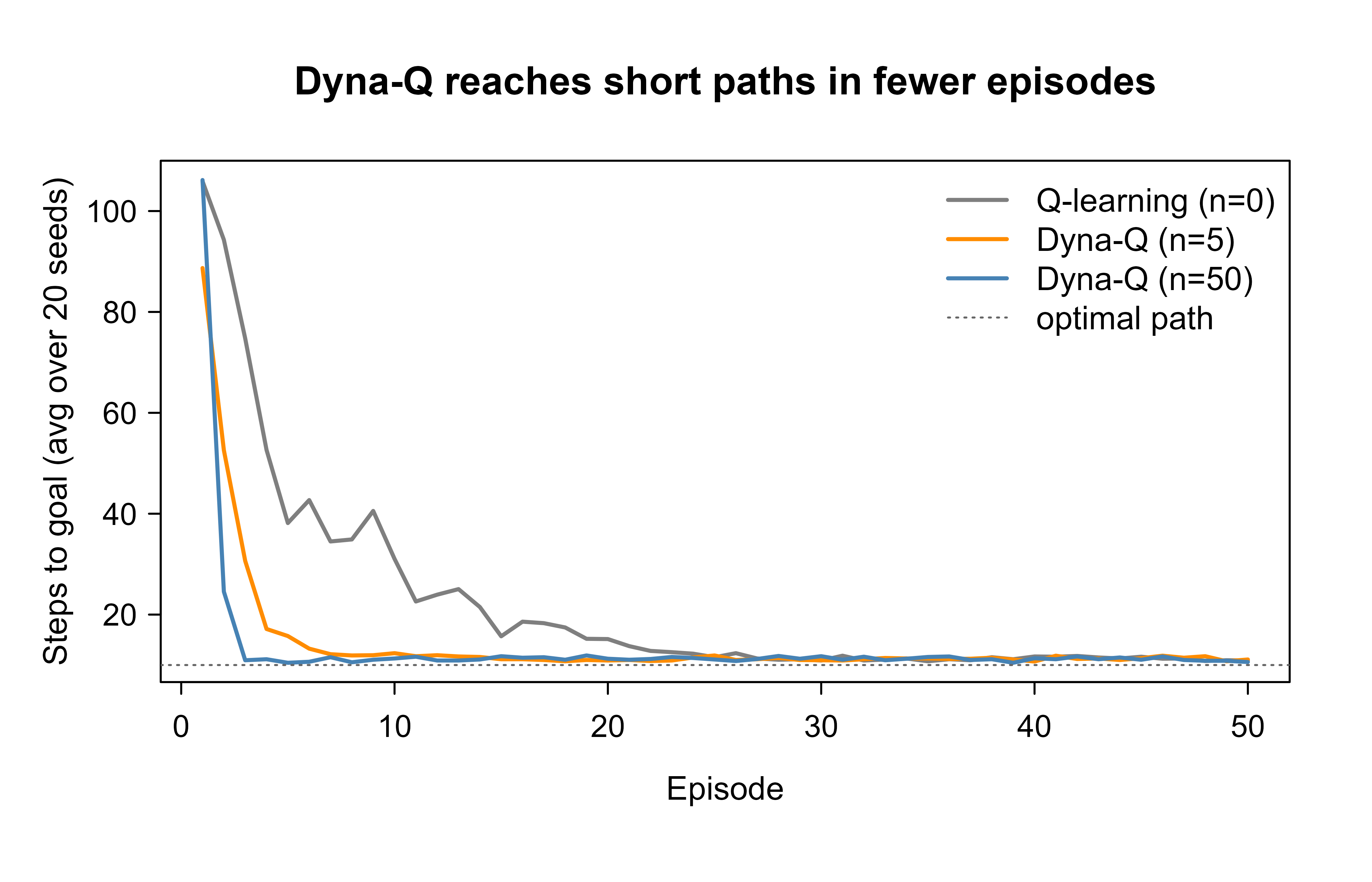
The table shows the headline result: in the first five episodes the Dyna-Q agents already take far fewer steps than plain Q-learning, because planning has propagated value information across the grid that Q-learning would only reach after many more real episodes. Figure 68.1 makes the same point visually with the full learning curves.

matplot(seq_len(n_episodes), avg_steps, type = "l", lty = 1, lwd = 2,
        col = c("grey50", "darkorange", "steelblue"),
        xlab = "Episode", ylab = "Steps to goal (avg over 20 seeds)",
        main = "Dyna-Q reaches short paths in fewer episodes")
abline(h = optimal_path, lty = 3, col = "grey40")
legend("topright", legend = c(colnames(avg_steps), "optimal path"),
       col = c("grey50", "darkorange", "steelblue", "grey40"),
       lty = c(1, 1, 1, 3), lwd = c(2, 2, 2, 1), bty = "n")

Figure 68.1: Steps to reach the goal per episode, averaged over 20 seeds, for plain Q-learning and two Dyna-Q agents. Lower is better. More planning steps per real step (larger n) collapses the steps-to-goal much faster, showing the sample-efficiency gain of model-based planning. All methods converge to the near-optimal path length, but Dyna-Q gets there in a fraction of the real experience.

The gap between the grey curve (no planning) and the blue curve (50 planning steps) is the sample-efficiency payoff in one picture. Plain Q-learning spends its early episodes wandering, because a single real transition only updates one cell of the Q-table and value information crawls outward one episode at a time. Dyna-Q replays the same handful of real transitions dozens of times per step, so within a few episodes the learned value has already flowed back from the goal across the reachable grid. Because this gridworld is deterministic and stationary, the learned model is exactly correct, so Dyna-Q here pays no model-bias cost: it is pure upside. In a noisy or changing environment the planning updates would inherit the model’s errors, which is the tradeoff the previous section warned about.

Note

Notice that all three methods converge to roughly the same final path length. Model-based planning does not find a better policy than model-free learning in the limit; both converge to the optimum on a problem this small. What planning buys is speed of convergence in real experience. When real experience is the scarce resource, that is the entire game.

68.6 Practical guidance and pitfalls

Model-based RL projects fail in characteristic ways, and most failures trace back to the bias-efficiency tradeoff. The following points collect the lessons that save the most time, roughly in the order you will meet them.

Start by asking whether you even need a model. If real interaction is cheap and plentiful (a fast simulator, a logged dataset large enough for offline learning, Chapter 69), a well-tuned model-free method is simpler to build and has no model-bias failure mode. Reach for model-based methods when real interaction is the bottleneck: physical robots, live systems with real users or real money, or any setting where each sample is slow or costly.

When you do learn a model, treat model error as the central risk, not an afterthought. Validate the model the way you would validate any predictive model: hold out transitions and check one-step prediction accuracy, and watch multi-step rollout accuracy, which degrades faster. Prefer an ensemble of models so that disagreement among them flags states where the model is uncertain, and avoid planning into regions where the ensemble disagrees.

Keep the planning horizon honest. The \((1-\gamma)^{-2}\) amplification in the simulation lemma is not just theory: planning many steps deep against an imperfect model reliably produces overconfident, wrong policies. Short rollouts that hand off to a learned value estimate (as in MCTS with a value network, or model-based methods that use the model only for a few steps) are far more robust than long open-loop rollouts.

Refit the model continually and watch for nonstationarity. Dyna-Q’s stored model goes stale the moment the environment changes; if your world is nonstationary, add an exploration bonus for under-visited or long-unvisited state-action pairs (the Dyna-Q+ idea) so the agent keeps its model fresh where it matters. A model that was accurate last week is not evidence that it is accurate now.

Tune the planning budget against your compute, not blindly upward. In Dyna-Q the planning steps n trade real-sample efficiency for computation per step; past some point the extra planning updates have diminishing returns because the Q-table is already near-converged on the visited region. In MCTS the analogous dial is the simulation budget per decision and the UCT exploration constant \(c\): too small a \(c\) commits to a single line too early, too large a \(c\) spreads simulations thinly and weakens the recommendation.

Tip

Get a tabular, deterministic version working first, exactly as in the demo above, where the learned model is provably correct and any failure is in your algorithm rather than your model. Only then introduce a learned function-approximation model and the bias problems that come with it. If Dyna-Q cannot beat Q-learning on a 6 by 6 grid, the bug is in the code, not the idea.

To summarize in one line: model-based RL learns or assumes a model of transitions and rewards and plans with it, trading the risk of model bias for a large gain in sample efficiency. Dyna-Q shows the gain cleanly by reusing each real transition for many planning updates, MCTS shows how to plan selectively in spaces too large to enumerate, and the simulation lemma explains why aggressive planning against a flawed model is the failure mode to guard against.

68.7 Further reading

• Sutton and Barto (2018), Reinforcement Learning: An Introduction (2nd ed.). The standard reference; Chapter 8 covers planning, Dyna, and the integration of model-based and model-free methods in full.
• Sutton (1990), Integrated architectures for learning, planning, and reacting based on approximating dynamic programming. The original Dyna paper.
• Kocsis and Szepesvari (2006), Bandit based Monte-Carlo planning. The paper introducing UCT.
• Coulom (2006), Efficient selectivity and backup operators in Monte-Carlo tree search. An early formulation of MCTS.
• Auer, Cesa-Bianchi, and Fischer (2002), Finite-time analysis of the multiarmed bandit problem. The UCB1 rule underlying UCT.
• Kearns and Singh (2002), Near-optimal reinforcement learning in polynomial time. The simulation-lemma analysis of model error.
• Moore and Atkeson (1993), Prioritized sweeping: reinforcement learning with less data and less time. The prioritized-sweeping variant of model-based planning.
• Strens (2000), A Bayesian framework for reinforcement learning. Posterior sampling (PSRL) using the Dirichlet posterior over transition models.
• Grimm, Barreto, Singh, and Silver (2020), The value equivalence principle for model-based reinforcement learning. Why a model need only be accurate for the value functions the agent computes.
• Silver et al. (2016), Mastering the game of Go with deep neural networks and tree search. MCTS combined with learned policy and value networks.
• Silver et al. (2017), Mastering the game of Go without human knowledge. AlphaGo Zero, learning the model-guided search from self-play alone.