62  Adversarial Learning

A well-trained classifier can reach high accuracy on a held-out test set and still be brittle in a way that ordinary evaluation never reveals. Take an image that the model labels “panda” with high confidence, add a perturbation so small that no human notices any change, and the same model now says “gibbon” with even higher confidence. The perturbation is not noise in the colloquial sense; it is a carefully chosen direction in input space that the model’s own gradient points to. This phenomenon, documented by Szegedy et al. (2014) and Goodfellow, Shlens, and Szegedy (2015), is the entry point to adversarial learning.

The name covers two ideas that share a mathematical core but solve different problems. The first is adversarial robustness: how do we attack a model with tiny input perturbations, and how do we defend against such attacks? This matters most for security-critical systems, spam filters, malware detectors, fraud scoring, and any model whose inputs are supplied by a party who benefits from fooling it. The second is adversarial training as a learning objective, where two models compete in a game. The generator-versus-discriminator setup behind generative adversarial networks is the famous case, and the same minimax structure reappears in domain-adversarial training for domain adaptation.

What ties the two together is a single optimization pattern: one player tries to minimize a loss while another tries to maximize it. In the robustness story the maximizing player is an attacker perturbing inputs; in the GAN story it is a discriminator trying to expose fakes. Once you see the minimax skeleton, attacks, defenses, and generative training all read as instances of the same game.

Intuition

A model that is accurate on average can still have a decision boundary that passes very close to many test points. “Close” is measured in input space, where a human’s notion of similarity and the model’s notion can diverge sharply. Adversarial examples live in that gap.

62.1 Adversarial examples and the geometry of brittleness

Fix a classifier \(f_\theta\) with parameters \(\theta\) that maps an input \(x \in \mathbb{R}^d\) to class scores, and let \(L(\theta, x, y)\) be the loss for the true label \(y\) (for instance cross-entropy). An adversarial example is a perturbed input \(x' = x + \delta\) that the model misclassifies, subject to a constraint that keeps the perturbation small:

\[ \max_{\delta}\; L(\theta, x + \delta, y) \quad\text{subject to}\quad \lVert \delta \rVert_p \le \epsilon . \]

The norm \(\lVert \cdot \rVert_p\) defines what “small” means. The \(\ell_\infty\) norm, \(\lVert \delta \rVert_\infty = \max_i |\delta_i|\), caps how much any single feature may move and is the most common choice for images. The \(\ell_2\) norm caps the total Euclidean size of the perturbation. The budget \(\epsilon\) is the radius of the allowed region around \(x\).

Why does such a \(\delta\) exist at all, and why is it often tiny? The short answer from Goodfellow, Shlens, and Szegedy (2015) is that high-dimensional models behave locally like linear functions. Suppose \(f\) scores a class as \(w^\top x + b\). Then perturbing \(x\) by \(\delta\) changes the score by \(w^\top \delta\). To push the score as far as possible under an \(\ell_\infty\) budget \(\epsilon\), set each coordinate of \(\delta\) to \(\epsilon \cdot \operatorname{sign}(w_i)\), giving a change of \(\epsilon \sum_i |w_i| = \epsilon \lVert w \rVert_1\). In \(d\) dimensions this grows with \(d\), so even a microscopic per-feature change \(\epsilon\) accumulates into a large swing in the score. Brittleness is partly a consequence of dimensionality, not just of model pathology.

Key idea

Many tiny coordinated nudges, each below the threshold of notice, sum to a large movement of the model’s score. The attacker spends a small budget per feature and is repaid in proportion to the dimension.

62.1.1 The fast gradient sign method

The fast gradient sign method (FGSM) turns the linear argument into a one-step attack. Linearize the loss around \(x\) using its gradient \(g = \nabla_x L(\theta, x, y)\). To first order, \(L(\theta, x + \delta, y) \approx L(\theta, x, y) + g^\top \delta\). Maximizing \(g^\top \delta\) under \(\lVert \delta \rVert_\infty \le \epsilon\) has the closed-form solution

\[ \delta^{\mathrm{FGSM}} = \epsilon \cdot \operatorname{sign}\!\big(\nabla_x L(\theta, x, y)\big), \qquad x' = x + \delta^{\mathrm{FGSM}} . \]

The sign function appears because, coordinate by coordinate, the largest contribution to \(g^\top \delta\) within \([-\epsilon, \epsilon]\) comes from moving each feature to the edge of its allowed range in the direction that increases the loss. FGSM is a single gradient evaluation, which is what makes it fast and a standard baseline.

The closed form is an instance of a general fact about linear maximization over a norm ball. For a fixed gradient \(g\), the linearized inner problem \(\max_{\lVert \delta \rVert_p \le \epsilon} g^\top \delta\) is solved by Hölder’s inequality, \(g^\top \delta \le \lVert g \rVert_q \lVert \delta \rVert_p\) with the dual exponent \(1/p + 1/q = 1\), and the bound is attained, so

\[ \max_{\lVert \delta \rVert_p \le \epsilon} g^\top \delta = \epsilon\, \lVert g \rVert_q , \qquad \tfrac{1}{p} + \tfrac{1}{q} = 1 . \tag{62.1}\]

The maximizer is the perturbation that aligns \(\delta\) with \(g\) in the geometry dual to \(\ell_p\). Working out the three cases used in practice:

• \(p = \infty\) (dual \(q = 1\)): equality in Hölder holds when each coordinate satisfies \(\delta_i = \epsilon\,\operatorname{sign}(g_i)\), recovering FGSM with value \(\epsilon \lVert g \rVert_1\).
• \(p = 2\) (dual \(q = 2\)): the maximizer is \(\delta = \epsilon\, g / \lVert g \rVert_2\), the normalized-gradient step, with value \(\epsilon \lVert g \rVert_2\).
• \(p = 1\) (dual \(q = \infty\)): the maximizer puts the entire budget on the single largest-magnitude coordinate, \(\delta = \epsilon\,\operatorname{sign}(g_{i^\star})\, e_{i^\star}\) with \(i^\star = \arg\max_i |g_i|\), a one-feature attack with value \(\epsilon \lVert g \rVert_\infty\).

This unifies the attack across norms: the worst-case first-order loss increase under an \(\ell_p\) budget is \(\epsilon \lVert \nabla_x L \rVert_q\), and the direction is read off from the equality condition in Equation 62.1.

Adversarial training as a gradient-norm penalty

Substituting the linearized worst case back into the robust objective exposes adversarial training as implicit regularization. To first order, \(\max_{\lVert \delta \rVert_p \le \epsilon} L(\theta, x+\delta, y) \approx L(\theta, x, y) + \epsilon \lVert \nabla_x L(\theta, x, y) \rVert_q\), so the inner maximization adds a penalty on the dual norm of the input gradient:

\[ \min_\theta\; \mathbb{E}_{(x,y)}\!\Big[\, L(\theta, x, y) + \epsilon \,\lVert \nabla_x L(\theta, x, y) \rVert_q \,\Big]. \tag{62.2}\]

Robust training therefore prefers parameters where the loss is flat in input space. The exact equivalence holds only in the linear regime; curvature makes the true robust loss larger than this first-order surrogate, which is precisely why one-step FGSM training can underprepare a model for multi-step attacks.

62.1.2 Projected gradient descent attacks

FGSM takes one big step along a linearized loss. When the loss is genuinely curved, one step overshoots or underexploits. Projected gradient descent (PGD), the attack studied by Madry et al. (2018), iterates small steps and projects back into the allowed region after each:

\[ x^{(t+1)} = \Pi_{\mathcal{B}_\epsilon(x)}\!\Big( x^{(t)} + \alpha \cdot \operatorname{sign}\!\big(\nabla_x L(\theta, x^{(t)}, y)\big) \Big), \]

where \(\alpha\) is the step size, \(\mathcal{B}_\epsilon(x) = \{ x' : \lVert x' - x \rVert_\infty \le \epsilon \}\) is the \(\ell_\infty\) ball of radius \(\epsilon\) around the clean input, and \(\Pi\) clips each coordinate back into that ball. Usually \(x^{(0)}\) is a random point inside the ball, which helps escape flat regions. PGD with enough steps is treated as a strong first-order attack: if a defense survives PGD, it has cleared a meaningful bar, though not a proof of security.

PGD is projected gradient ascent on the constrained inner problem \(\max_{x' \in \mathcal{B}_\epsilon(x)} L(\theta, x', y)\), with one twist: under the \(\ell_\infty\) norm the ascent step uses the sign of the gradient rather than the gradient itself. This is the steepest-ascent direction in the \(\ell_\infty\) geometry, exactly as in Equation 62.1, so each PGD step is an FGSM step of size \(\alpha\) followed by a projection. The projection \(\Pi_{\mathcal{B}_\epsilon(x)}\) is the Euclidean nearest point in the ball and has a closed form for the common norms. For \(\ell_\infty\) it is coordinatewise clipping,

\[ \big[\Pi_{\mathcal{B}_\epsilon^\infty(x)}(u)\big]_i = x_i + \operatorname{clip}\big(u_i - x_i,\, -\epsilon,\, \epsilon\big) = \min\!\big(\max(u_i,\, x_i - \epsilon),\, x_i + \epsilon\big) , \]

and for \(\ell_2\) it shrinks the deviation toward the ball,

\[ \Pi_{\mathcal{B}_\epsilon^2(x)}(u) = x + (u - x)\,\min\!\Big(1,\ \frac{\epsilon}{\lVert u - x \rVert_2}\Big) . \]

For image inputs one composes this with a clip to the valid pixel range, an intersection of two convex sets handled by clipping in sequence. Choosing \(\alpha < \epsilon\) and taking several steps lets PGD trace the curvature of \(L\) that a single FGSM step linearizes away, which is why PGD with \(K\) steps dominates FGSM as the inner solver.

Warning

A defense that lowers the gradient signal without changing the decision boundary can defeat FGSM and PGD by gradient masking, giving a false sense of safety. Such defenses fall to attacks that estimate gradients differently or transfer examples from a substitute model (Athalye, Carlini, and Wagner (2018)). Always report the attack used and its budget.

62.2 Adversarial training as a defense

If the attacker solves an inner maximization, the natural defense is to train against the worst case. Madry et al. (2018) frame robust learning as a saddle-point problem:

\[ \min_{\theta}\; \mathbb{E}_{(x,y)}\!\left[\; \max_{\lVert \delta \rVert_p \le \epsilon} L(\theta, x + \delta, y) \;\right]. \]

The inner \(\max\) finds the strongest perturbation for the current model; the outer \(\min\) updates parameters to be robust to it. In practice you approximate the inner problem with FGSM or PGD, generate adversarial inputs on each minibatch, and train on them (often mixed with clean inputs). This is adversarial training, and it remains one of the few defenses that holds up under careful evaluation.

62.2.1 Why training on the attacked point is the right gradient

The saddle-point objective hides a subtlety: the outer loss \(\phi(\theta) = \max_{\lVert \delta \rVert_p \le \epsilon} L(\theta, x + \delta, y)\) is itself a maximization, so how do we differentiate it with respect to \(\theta\)? Danskin’s theorem answers this. If \(L(\theta, x+\delta, y)\) is differentiable in \(\theta\), the constraint set \(\{\delta : \lVert \delta \rVert_p \le \epsilon\}\) is compact, and the inner maximizer is unique at \(\delta^\star(\theta) = \arg\max_{\lVert \delta \rVert_p \le \epsilon} L(\theta, x+\delta, y)\), then the maximized loss is differentiable and its gradient is the gradient of \(L\) evaluated at the maximizer, with the dependence of \(\delta^\star\) on \(\theta\) ignored:

\[ \nabla_\theta\, \phi(\theta) = \nabla_\theta\, L\big(\theta,\, x + \delta^\star(\theta),\, y\big) . \tag{62.3}\]

The result is intuitive once stated: at an interior maximizer the partial derivative of \(L\) with respect to \(\delta\) vanishes (or is orthogonal to the active constraint), so the chain-rule term \(\nabla_\delta L \cdot \partial \delta^\star/\partial \theta\) contributes nothing, leaving only the explicit dependence on \(\theta\). Madry et al. (2018) invoke Equation 62.3 to justify the standard recipe: find a strong \(\delta^\star\) with PGD, then take an ordinary gradient step on the loss at the perturbed point. The theorem requires the inner problem to be solved to optimality; PGD only approximates it, so the descent direction is approximate, which is one reason robust training is noisier and slower to converge than standard training.

Robustness has a price. Pushing the decision boundary away from the data along every direction the attacker might exploit can lower clean accuracy, the robustness-accuracy tradeoff analyzed by Tsipras et al. (2019). Robust models also tend to need more data and more capacity. The right operating point depends on the threat: a fraud model facing adaptive adversaries may accept a clean-accuracy hit that a benign recommender would not.

62.2.2 A model where robustness and accuracy genuinely conflict

The tradeoff is not merely empirical; Tsipras et al. (2019) construct a distribution where the most accurate classifier is provably the least robust. Let the label \(y \in \{-1, +1\}\) be balanced, and let the features be one strongly correlated coordinate plus \(d\) weakly correlated coordinates:

\[ x_1 = \begin{cases} +y & \text{w.p. } p \\ -y & \text{w.p. } 1-p \end{cases}, \qquad x_j \sim \mathcal{N}(\eta\, y,\, 1), \quad j = 2, \dots, d+1 , \]

with \(p\) slightly above \(\tfrac{1}{2}\) (say \(p = 0.95\)) and \(\eta = \Theta(1/\sqrt{d})\) small. Each weak feature carries little signal, but averaging \(d\) of them concentrates: \(\bar{x} = \tfrac{1}{d}\sum_{j\ge 2} x_j \sim \mathcal{N}(\eta y, 1/d)\), so the classifier \(\operatorname{sign}(\bar{x})\) achieves a high constant accuracy \(\Phi(\eta\sqrt{d}) = \Phi(\Theta(1))\), independent of \(d\). With a suitable constant in \(\eta = c/\sqrt{d}\) (for example \(\eta = 4/\sqrt{d}\), giving \(\Phi(4) \approx 0.99997\)), this beats the \(95\%\) ceiling of the robust feature \(x_1\). The scaling \(\eta = \Theta(1/\sqrt{d})\) is precisely what keeps this accuracy constant in \(d\) while keeping the \(\epsilon = 2\eta\) budget small (vanishing as \(d\) grows). The standard, most-accurate classifier therefore leans on the weak features.

Now give an \(\ell_\infty\) adversary budget \(\epsilon = 2\eta\). The adversary shifts every weak coordinate by \(-2\eta y\), flipping each \(x_j\) from mean \(\eta y\) to mean \(-\eta y\), which inverts the sign of \(\bar{x}\) in expectation and drives the accuracy of the weak-feature classifier toward \(0\). The robust feature \(x_1\) cannot be flipped by a small \(\ell_\infty\) perturbation (it is already \(\pm 1\) and \(\epsilon < 1\)), so a classifier that ignores the weak features and uses only \(x_1\) keeps accuracy \(p\) under attack. The conflict is fundamental to this distribution: maximizing clean accuracy forces reliance on features that an adversary can overturn, while robustness forces the model to discard exactly those features. No amount of capacity or data removes the gap, because it lives in the data-generating process, not in the optimizer.

When to use this

Reach for adversarial training when inputs come from a party who gains by fooling the model, or when a wrong prediction on a perturbed input is costly (security, safety, finance). For ordinary i.i.d. deployment with no adversary, the clean-accuracy cost is usually not worth paying.

62.3 A runnable demo: attacking and defending a linear classifier

The geometry is easiest to see with a model whose gradient is exact rather than approximate. We use logistic regression, where the loss gradient with respect to the input has a clean closed form, so FGSM is not an approximation but the genuine worst-case linear perturbation. We simulate two Gaussian classes, fit the classifier, build FGSM perturbations, and measure how accuracy collapses. Then we retrain on adversarially perturbed data and measure recovery.

For logistic regression the predicted probability is \(\sigma(z) = 1 / (1 + e^{-z})\) with \(z = \beta_0 + x^\top \beta\). The cross-entropy loss for a label \(y \in \{0,1\}\) has input gradient

\[ \nabla_x L = \big(\sigma(z) - y\big)\, \beta , \]

so the FGSM perturbation is \(\delta = \epsilon \cdot \operatorname{sign}\!\big((\sigma(z) - y)\,\beta\big)\). Because \(\operatorname{sign}((\sigma(z)-y)\beta) = \operatorname{sign}(\sigma(z)-y)\cdot \operatorname{sign}(\beta)\), the attack simply moves every feature by \(\pm\epsilon\) toward the wrong class. The direction is the same for every point of a given class, which is exactly the linear picture from above.

set.seed(1301)

# Two Gaussian classes in 2-D with overlap so the boundary is non-trivial.
n <- 400
mu0 <- c(-1.0, -1.0)
mu1 <- c( 1.0,  1.0)
Sigma <- matrix(c(1, 0.3, 0.3, 1), 2, 2)

rmvn <- function(n, mu, Sigma) {
  L <- chol(Sigma)
  matrix(rnorm(n * 2), n, 2) %*% L + matrix(mu, n, 2, byrow = TRUE)
}

X0 <- rmvn(n / 2, mu0, Sigma)
X1 <- rmvn(n / 2, mu1, Sigma)
X  <- rbind(X0, X1)
y  <- c(rep(0, n / 2), rep(1, n / 2))

# Train / test split.
idx   <- sample(seq_len(n), size = floor(0.6 * n))
Xtr   <- X[idx, ];  ytr <- y[idx]
Xte   <- X[-idx, ]; yte <- y[-idx]

sigmoid <- function(z) 1 / (1 + exp(-z))

# Fit logistic regression (clean model).
df_tr <- data.frame(x1 = Xtr[, 1], x2 = Xtr[, 2], y = ytr)
clean_fit <- glm(y ~ x1 + x2, data = df_tr, family = binomial())
beta  <- coef(clean_fit)[c("x1", "x2")]
beta0 <- coef(clean_fit)[["(Intercept)"]]

The attack function below builds the FGSM perturbation for a batch of points. Each row of the input matrix is nudged by \(\epsilon\) in the sign direction that raises its loss.

# FGSM perturbation for logistic regression, exact input gradient.
fgsm <- function(Xmat, yvec, beta, beta0, epsilon) {
  z    <- as.numeric(beta0 + Xmat %*% beta)
  p    <- sigmoid(z)
  # grad_x L = (p - y) * beta, broadcast over rows.
  grad <- outer(p - yvec, beta)              # n x 2
  Xmat + epsilon * sign(grad)
}

predict_label <- function(Xmat, beta, beta0) {
  as.integer(sigmoid(as.numeric(beta0 + Xmat %*% beta)) > 0.5)
}

epsilon <- 1.0

# Clean and adversarial test accuracy for the clean model.
acc <- function(pred, truth) mean(pred == truth)

clean_acc_clean_model <- acc(predict_label(Xte, beta, beta0), yte)
Xte_adv <- fgsm(Xte, yte, beta, beta0, epsilon)
adv_acc_clean_model <- acc(predict_label(Xte_adv, beta, beta0), yte)

Now we apply the defense. We augment the training set with FGSM perturbations of the training points (generated from the clean model’s parameters), refit, and re-evaluate against both clean and freshly attacked test data. The freshly attacked test set uses the defended model’s own gradient, so the attacker adapts to the new model rather than reusing stale perturbations.

# Adversarial training: augment with FGSM-perturbed training points.
Xtr_adv <- fgsm(Xtr, ytr, beta, beta0, epsilon)
df_aug  <- data.frame(
  x1 = c(Xtr[, 1], Xtr_adv[, 1]),
  x2 = c(Xtr[, 2], Xtr_adv[, 2]),
  y  = c(ytr, ytr)
)
robust_fit <- glm(y ~ x1 + x2, data = df_aug, family = binomial())
rbeta  <- coef(robust_fit)[c("x1", "x2")]
rbeta0 <- coef(robust_fit)[["(Intercept)"]]

clean_acc_robust_model <- acc(predict_label(Xte, rbeta, rbeta0), yte)
# Attacker adapts to the defended model's gradient.
Xte_adv_r <- fgsm(Xte, yte, rbeta, rbeta0, epsilon)
adv_acc_robust_model <- acc(predict_label(Xte_adv_r, rbeta, rbeta0), yte)

results <- data.frame(
  Model = c("Standard (clean training)", "Adversarial training"),
  `Clean accuracy` = round(c(clean_acc_clean_model, clean_acc_robust_model), 3),
  `Adversarial accuracy` = round(c(adv_acc_clean_model, adv_acc_robust_model), 3),
  check.names = FALSE
)

Table 62.1 reports the four numbers. The standard model keeps high clean accuracy but its adversarial accuracy falls sharply: a per-feature nudge of \(\epsilon = 1\) flips a large share of test predictions. Adversarial training trades a little clean accuracy for a large gain in adversarial accuracy, the robustness-accuracy tradeoff in miniature.

knitr::kable(
  results,
  caption = "Clean versus adversarial test accuracy for a standard logistic-regression classifier and the same classifier after adversarial training (FGSM augmentation, epsilon = 1.0). Adversarial accuracy is measured against perturbations adapted to each model."
)

Table 62.1: Clean versus adversarial test accuracy for a standard logistic-regression classifier and the same classifier after adversarial training (FGSM augmentation, epsilon = 1.0). Adversarial accuracy is measured against perturbations adapted to each model.

Model	Clean accuracy	Adversarial accuracy
Standard (clean training)	0.894	0.494
Adversarial training	0.912	0.512

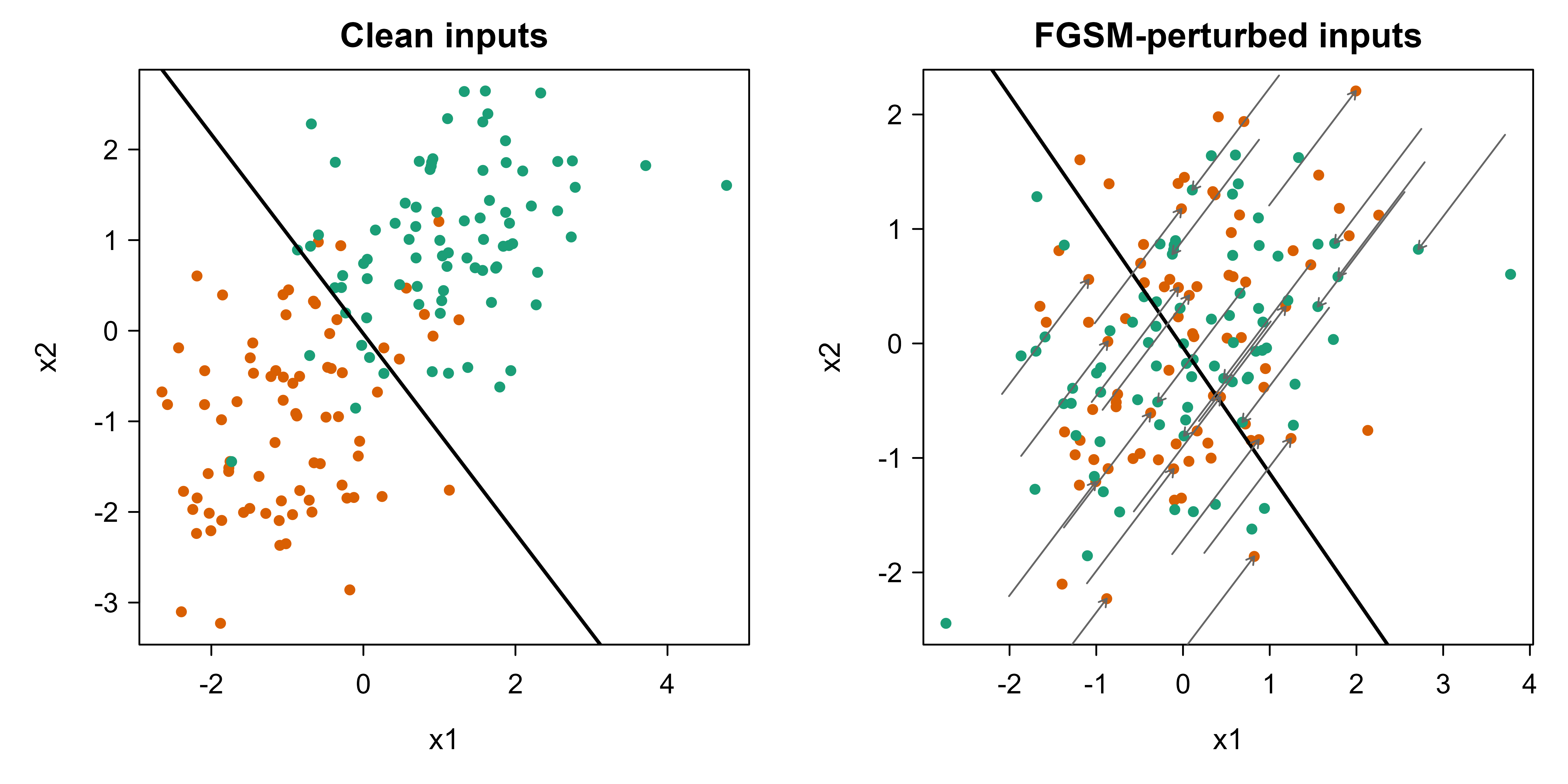
Figure 62.1 shows the geometry. The left panel plots the clean test points with the standard model’s decision boundary. The right panel shows the same points after the FGSM attack: every class-1 point slides down-left and every class-0 point slides up-right, both toward the boundary, and many cross it. The arrows in the right panel trace the perturbation applied to a sample of points.

op <- par(mfrow = c(1, 2), mar = c(4, 4, 2, 1))

# Boundary: beta0 + b1*x1 + b2*x2 = 0  =>  x2 = -(beta0 + b1*x1)/b2
abline_for <- function(b0, b) c(intercept = unname(-b0 / b[2]), slope = unname(-b[1] / b[2]))

cols <- ifelse(yte == 1, "#1b9e77", "#d95f02")

# Panel 1: clean
plot(Xte[, 1], Xte[, 2], col = cols, pch = 19, cex = 0.7,
     xlab = "x1", ylab = "x2", main = "Clean inputs")
ln <- abline_for(beta0, beta)
abline(a = ln["intercept"], b = ln["slope"], lwd = 2)

# Panel 2: adversarial
plot(Xte_adv[, 1], Xte_adv[, 2], col = cols, pch = 19, cex = 0.7,
     xlab = "x1", ylab = "x2", main = "FGSM-perturbed inputs")
abline(a = ln["intercept"], b = ln["slope"], lwd = 2)
samp <- sample(seq_len(nrow(Xte)), 25)
arrows(Xte[samp, 1], Xte[samp, 2],
       Xte_adv[samp, 1], Xte_adv[samp, 2],
       length = 0.05, col = "grey40")

par(op)

Figure 62.1: Left: clean test points and the standard model’s linear decision boundary. Right: the same points after the FGSM attack (epsilon = 1.0); arrows show the perturbation on a sample of points, which pushes each class uniformly toward and across the boundary.

The lesson generalizes past logistic regression. Any model with a usable input gradient, the neural networks of Chapter 15 foremost among them, admits FGSM and PGD attacks, and adversarial training is the corresponding defense. The linear case just lets us see the closed form and the uniform per-class shift that more complex models hide.

The optimality claim in Equation 62.1 is easy to confirm numerically: the sign perturbation should attain the bound \(\epsilon \lVert g \rVert_1\) exactly, and no random perturbation inside the \(\ell_\infty\) ball should beat it.

set.seed(7)
g  <- rnorm(50)          # an arbitrary loss gradient
eps <- 0.1

# Closed-form optimum from the Holder argument.
opt_fgsm  <- sum(g * (eps * sign(g)))   # should equal eps * ||g||_1
bound     <- eps * sum(abs(g))

# Best of many random perturbations inside the L-infinity ball.
rand_best <- max(replicate(100000, {
  d <- runif(length(g), -eps, eps)
  sum(g * d)
}))

c(fgsm_value = opt_fgsm, holder_bound = bound, random_best = rand_best)
#>   fgsm_value holder_bound  random_best 
#>     4.085459     4.085459     1.952219

The FGSM value equals the Hölder bound to machine precision, and the best of 100000 random perturbations falls short of it, confirming that the sign step is the exact maximizer of the linearized loss under an \(\ell_\infty\) budget.

62.4 The adversarial game behind GANs

The minimax pattern that defines robust training is the same one that drives generative adversarial networks (see the generative models chapter (Chapter 42) for the full treatment). A generator \(G\) maps noise \(z \sim p_z\) to samples \(G(z)\), and a discriminator \(D\) outputs the probability that an input is real rather than generated. They play

\[ \min_{G}\; \max_{D}\; \mathbb{E}_{x \sim p_{\mathrm{data}}}\!\big[\log D(x)\big] + \mathbb{E}_{z \sim p_z}\!\big[\log\big(1 - D(G(z))\big)\big]. \]

The discriminator maximizes its ability to separate real from fake; the generator minimizes that ability by producing samples the discriminator cannot flag. Compare this to the robustness saddle point: there the inner \(\max\) is over input perturbations and the outer \(\min\) is over model parameters; here the inner \(\max\) is over the discriminator and the outer \(\min\) is over the generator. Same skeleton, different players. Goodfellow et al. (2014) show that at the global optimum the generator reproduces the data distribution and the discriminator is reduced to guessing, \(D \equiv \tfrac{1}{2}\).

The proof of that statement is a short two-step argument worth seeing, because it pins down exactly what the generator is minimizing. Let \(p_g\) be the distribution of \(G(z)\) and write the objective as \(V(G, D) = \int p_{\mathrm{data}}(x) \log D(x) + p_g(x) \log(1 - D(x))\, dx\). For fixed \(G\), the integrand at each \(x\) has the form \(a \log D + b \log(1 - D)\) with \(a = p_{\mathrm{data}}(x)\) and \(b = p_g(x)\); setting the derivative \(a/D - b/(1-D) = 0\) gives the optimal discriminator pointwise,

\[ D^\star(x) = \frac{p_{\mathrm{data}}(x)}{p_{\mathrm{data}}(x) + p_g(x)} . \tag{62.4}\]

Substituting \(D^\star\) back collapses the inner maximum into a divergence between the two distributions. Using \(\log 2\) to recenter,

\[ \begin{aligned} V(G, D^\star) &= \mathbb{E}_{p_{\mathrm{data}}}\!\Big[\log \tfrac{p_{\mathrm{data}}}{p_{\mathrm{data}} + p_g}\Big] + \mathbb{E}_{p_g}\!\Big[\log \tfrac{p_g}{p_{\mathrm{data}} + p_g}\Big] \\ &= -\log 4 + \mathrm{KL}\!\Big(p_{\mathrm{data}} \,\Big\|\, \tfrac{p_{\mathrm{data}} + p_g}{2}\Big) + \mathrm{KL}\!\Big(p_g \,\Big\|\, \tfrac{p_{\mathrm{data}} + p_g}{2}\Big) \\ &= -\log 4 + 2\,\mathrm{JSD}(p_{\mathrm{data}} \,\|\, p_g) , \end{aligned} \tag{62.5}\]

where \(\mathrm{JSD}\) is the Jensen-Shannon divergence. Because \(\mathrm{JSD} \ge 0\) with equality iff \(p_g = p_{\mathrm{data}}\), the generator’s minimization of Equation 62.5 is uniquely solved at \(p_g = p_{\mathrm{data}}\), at which point Equation 62.4 gives \(D^\star \equiv \tfrac{1}{2}\) and the game value is \(-\log 4\). This also explains a notorious failure mode: where \(p_{\mathrm{data}}\) and \(p_g\) have disjoint supports the JSD is constant at \(\log 2\), so its gradient vanishes and the generator receives no signal. That flat-gradient pathology motivated Wasserstein GANs, which replace the JSD with an earth-mover distance that varies smoothly even between non-overlapping distributions (see Chapter 42).

Note

The shared minimax form is more than an analogy. Both settings inherit the same difficulties: the inner problem is rarely solved exactly, the outer updates chase a moving target, and naive alternation can oscillate instead of converging. Techniques that stabilize one game often inform the other.

62.4.1 Domain-adversarial training

A third use of the same idea adapts a model trained on one data distribution (the source) to perform on a different but related one (the target), the problem of domain adaptation studied more broadly in the transfer and multi-task learning chapter (Chapter 54). Ganin et al. (2016) attach a domain classifier that tries to tell source features from target features, and train the feature extractor to fool it through a gradient-reversal layer. If a feature representation makes source and target indistinguishable, a label predictor trained on the source should transfer to the target. The objective again has the competing-players form: the feature extractor minimizes label loss while maximizing domain-classification loss, and the domain classifier does the opposite.

# Sketch of domain-adversarial training (requires a deep-learning backend, so eval=FALSE).
# feature_extractor: x -> h
# label_predictor:   h -> y_hat   (trained on labeled source only)
# domain_classifier: h -> d_hat   (real source vs target)
#
# Total loss = label_loss(label_predictor(h), y)            # minimized by extractor + predictor
#            - lambda * domain_loss(domain_classifier(h), d) # extractor MAXIMIZES this term
#
# The minus sign is implemented by a gradient-reversal layer: forward pass is identity,
# backward pass multiplies the gradient by -lambda before it reaches the feature extractor.

62.5 Practical guidance and pitfalls

Several recurring mistakes undermine work on adversarial robustness, and a few habits keep evaluations honest.

State the threat model before anything else. An attack is only meaningful relative to a norm, a budget \(\epsilon\), and an assumption about what the attacker knows. White-box attacks see the model’s gradients; black-box attacks do not and must transfer examples from a substitute or estimate gradients by queries. Reporting “robust accuracy” without the budget and access model is uninterpretable.

Do not trust a defense that only beats FGSM. A single gradient step is the weakest standard attack. Athalye, Carlini, and Wagner (2018) showed that many published defenses worked by obfuscating gradients, making the loss surface locally uninformative without moving the boundary, and collapsed under PGD or transfer attacks. Evaluate against a strong iterative attack with multiple random restarts, and be suspicious when robust accuracy is high but the loss gradient is near zero.

Budget the inner optimization realistically. PGD adversarial training multiplies training cost by the number of inner steps. Single-step adversarial training is cheaper but can suffer catastrophic overfitting, where robustness to multi-step attacks suddenly collapses mid-training. Monitor robust accuracy against a multi-step attack during training, not just the single-step proxy you train on.

Expect to pay for robustness. The robustness-accuracy tradeoff (Tsipras et al. (2019)) is real: clean accuracy usually drops, and robust models often need more data and capacity. Decide up front how much clean accuracy you are willing to trade, and tie that decision to the cost of an adversarial failure in your application.

Match the perturbation set to the real threat. The \(\ell_\infty\) ball is a mathematical convenience, not a model of every attacker. Real adversaries rotate images, paste stickers, paraphrase text, or change the timing of network packets, none of which is a small \(\ell_p\) perturbation. Robustness inside one ball does not imply robustness to transformations outside it.

For GAN-style training, watch for non-convergence and mode collapse, where the generator maps many noise vectors to a few outputs that happen to fool the current discriminator. These are the generative counterparts of the optimization instabilities that also afflict adversarial robustness, and they trace back to the same fact: nobody is solving the inner problem exactly.

62.6 Certified robustness: guarantees beyond empirical attacks

Empirical robustness against PGD is a lower bound on vulnerability: it tells you the model survived the attacks you tried, not that no attack exists. Certified defenses instead produce a provable radius \(r\) around an input within which the prediction cannot change. The most scalable certificate is randomized smoothing (Cohen, Rosenfeld, and Kolter (2019)). Given any base classifier \(h\), define the smoothed classifier

\[ \bar{h}(x) = \arg\max_{c}\; \mathbb{P}_{\eta \sim \mathcal{N}(0, \sigma^2 I)}\big[\, h(x + \eta) = c \,\big], \]

the majority vote of \(h\) under Gaussian noise. If the top class \(c_A\) has probability at least \(\underline{p_A}\) and the runner-up at most \(\overline{p_B}\) under the noise, then \(\bar{h}\) is constant, hence its prediction is certifiably unchanged, for every \(\ell_2\) perturbation of radius

\[ r = \frac{\sigma}{2}\Big(\Phi^{-1}(\underline{p_A}) - \Phi^{-1}(\overline{p_B})\Big), \tag{62.6}\]

where \(\Phi^{-1}\) is the standard-normal quantile function. The proof rests on the isoperimetric property of the Gaussian: shifting the noise distribution by \(\delta\) can change the probability of any half-space by at most an amount controlled by \(\Phi^{-1}\), so a margin in probability space translates into a margin in input space. In practice the two probabilities are estimated by Monte Carlo sampling of \(h(x + \eta)\) with a confidence correction, giving a high-probability certificate. The noise level \(\sigma\) is the central hyperparameter: larger \(\sigma\) certifies larger radii (Equation 62.6 scales with \(\sigma\)) but blurs the input and lowers clean accuracy, a direct dial on the robustness-accuracy tradeoff.

Certified versus empirical

Empirical robustness can only ever be falsified by a stronger attack; a certificate can only ever be loose, never wrong. The two are complementary: report PGD accuracy as an upper bound on robustness and a certified radius as a lower bound, and trust a defense most when the gap between them is small.

62.7 Cost, convergence, and hyperparameters at a glance

The dominant cost of robust training is the inner solver. Each PGD step is one forward-backward pass, so \(K\)-step PGD adversarial training costs roughly \(K + 1\) times standard training per minibatch (the \(+1\) for the outer parameter update). FGSM training costs about twice standard training. This sets the practical menu:

• Step size \(\alpha\) and steps \(K\) for the attack. A common rule is \(\alpha \approx 2.5\,\epsilon / K\) so the iterate can traverse the ball; \(K\) between \(7\) and \(40\) is typical for evaluation, fewer during training. More restarts reduce the chance of reporting an inflated robust accuracy from a bad random start.
• Budget \(\epsilon\). Set it from the threat, not from convenience. For \([0,1]\)-scaled images, \(\ell_\infty\) budgets of \(8/255\) are a community benchmark; there is nothing fundamental about that number.
• Catastrophic overfitting. Single-step training can show robust accuracy against PGD suddenly collapsing to near zero within one epoch while FGSM accuracy stays high. The cure is to monitor multi-step robust accuracy, add a random initialization to the FGSM step, or cap the step size; if it appears, fall back to a few PGD steps.
• Diagnosing gradient masking. If robust accuracy is high but (i) the loss gradient norm is near zero, (ii) iterative attacks do no better than single-step, (iii) unbounded \(\epsilon\) fails to drive accuracy to zero, or (iv) black-box transfer attacks beat white-box ones, the defense is likely obfuscating gradients rather than being robust (Athalye, Carlini, and Wagner (2018)). A correct defense should let an unbounded attacker eventually win.

62.8 Further reading

• Szegedy, Zaremba, Sutskever, Bruna, Erhan, Goodfellow, and Fergus (2013), the paper that first reported adversarial examples for neural networks.
• Goodfellow, Shlens, and Szegedy (2015), introducing the fast gradient sign method and the linear explanation of adversarial examples.
• Madry, Makelov, Schmidt, Tsipras, and Vladu (2018), the projected gradient descent attack and the saddle-point view of robust training.
• Tsipras, Santurkar, Engstrom, Turner, and Madry (2019), on the robustness-accuracy tradeoff.
• Athalye, Carlini, and Wagner (2018), on obfuscated gradients and how to evaluate defenses honestly.
• Goodfellow, Pouget-Abadie, Mirza, Xu, Warde-Farley, Ozair, Courville, and Bengio (2014), the original generative adversarial networks paper.
• Ganin, Ustinova, Ajakan, Germain, Larochelle, Laviolette, Marchand, and Lempitsky (2016), on domain-adversarial training of neural networks.
• Cohen, Rosenfeld, and Kolter (2019), on certified \(\ell_2\) robustness via randomized smoothing.

Athalye, Anish, Nicholas Carlini, and David Wagner. 2018. “Obfuscated Gradients Give a False Sense of Security.” In International Conference on Machine Learning (ICML).

Cohen, Jeremy M., Elan Rosenfeld, and J. Zico Kolter. 2019. “Certified Adversarial Robustness via Randomized Smoothing.” In International Conference on Machine Learning (ICML).

Ganin, Yaroslav, Evgeniya Ustinova, Hana Ajakan, Pascal Germain, Hugo Larochelle, Francois Laviolette, Mario Marchand, and Victor Lempitsky. 2016. “Domain-Adversarial Training of Neural Networks.” Journal of Machine Learning Research 17 (59): 1–35.

Goodfellow, Ian J., Jean Pouget-Abadie, Mehdi Mirza, Bing Xu, David Warde-Farley, Sherjil Ozair, Aaron Courville, and Yoshua Bengio. 2014. “Generative Adversarial Nets.” In Advances in Neural Information Processing Systems (NeurIPS).

Goodfellow, Ian J., Jonathon Shlens, and Christian Szegedy. 2015. “Explaining and Harnessing Adversarial Examples.” In International Conference on Learning Representations (ICLR).

Madry, Aleksander, Aleksandar Makelov, Ludwig Schmidt, Dimitris Tsipras, and Adrian Vladu. 2018. “Towards Deep Learning Models Resistant to Adversarial Attacks.” In International Conference on Learning Representations (ICLR).

Szegedy, Christian, Wojciech Zaremba, Ilya Sutskever, Joan Bruna, Dumitru Erhan, Ian Goodfellow, and Rob Fergus. 2014. “Intriguing Properties of Neural Networks.” In International Conference on Learning Representations (ICLR).

Tsipras, Dimitris, Shibani Santurkar, Logan Engstrom, Alexander Turner, and Aleksander Madry. 2019. “Robustness May Be at Odds with Accuracy.” In International Conference on Learning Representations (ICLR).