Most of this book asks a predictive question: given features \(X\), what is the best guess for an outcome \(Y\)? Causal machine learning asks a different question. If we intervene and set a treatment \(W\) to a particular value, how does \(Y\) change, and for whom does it change the most? Predicting who will buy a product is not the same as predicting who will buy because we sent them a coupon. The second question is the one that drives budgets, retention campaigns, pricing, and medical decisions, and it is the one a standard supervised model does not answer on its own.
This chapter connects the potential outcomes framework to the supervised learning machinery developed earlier in the book. The goal is heterogeneous treatment effect estimation: not a single average effect but a function that maps each unit’s features to its own expected effect. We cover meta-learners (S-, T-, and X-learners), causal forests, and double/debiased machine learning (DML), and then turn to uplift modeling, which is the applied targeting problem that these methods solve in marketing and operations.
Identification (the assumptions under which a causal effect can be recovered from observational data at all) was treated in detail in the first book of this series. Here we take identification as given and focus on estimation with flexible ML models. When the assumptions below feel unfamiliar, review the identification chapter of the first book.
Key idea
A predictive model ranks units by what will happen. A causal model ranks them by how much your action changes what happens. These two rankings can be almost unrelated, and confusing them is the single most common mistake in applied targeting.
By the end of the chapter you will be able to state the estimand (the CATE) precisely, choose among the main estimator families (meta-learners, causal forests, double/debiased ML), fit a working CATE estimator in R, and evaluate it honestly when the truth is unknown.
76.1 Where this fits in a modern ML/AI workflow
A typical ML workflow produces a scoring model: a churn score, a propensity score, a fraud score. Decisions then get made by thresholding that score. The hidden assumption is that the score ranks people by how much an action will help them. It usually does not. A customer with a 90% renewal probability may renew with or without a discount, so spending on them is wasted. A customer at 55% might be pushed over the line by the same discount. Causal ML estimates that push, the incremental effect, so that targeting spends the budget where it changes behavior.
In practice causal ML sits downstream of the same feature pipelines (Chapter 119), data warehouses, and experiment platforms (Chapter 115) that feed predictive models. The natural inputs are randomized experiments (A/B tests) or logged observational data with a known or estimable assignment mechanism. The outputs feed back into the same serving and decision layers: instead of scoring “probability of conversion,” you score “expected lift from the offer” and rank by that. Teams that already run experiments and have a feature store are well positioned, because the marginal cost is mostly modeling and validation, not new infrastructure.
When to use this
Reach for causal ML when a decision will act on the units being scored (send a coupon, schedule a call, prescribe a drug, choose a price). If the action is the same for everyone and you only need a forecast to plan capacity or set a threshold, a plain predictive model is simpler and usually enough.
76.2 Potential outcomes recap and CATE
We use the Neyman-Rubin potential outcomes model. For each unit \(i\) let \(W_i \in \{0, 1\}\) be a binary treatment (1 = treated, 0 = control), let \(X_i \in \mathbb{R}^p\) be pre-treatment covariates, and let \(Y_i(0)\) and \(Y_i(1)\) be the two potential outcomes, one for each treatment value. We observe only one of them, \[
Y_i = W_i \, Y_i(1) + (1 - W_i) \, Y_i(0),
\] which is the fundamental problem of causal inference: the other potential outcome is a counterfactual we never see for that unit.1
The unit-level treatment effect is \(\tau_i = Y_i(1) - Y_i(0)\). It is not identified for a single unit because one term is always missing. What we can identify, under the assumptions below, is the Conditional Average Treatment Effect (CATE), \[
\tau(x) = \mathbb{E}\!\left[\, Y_i(1) - Y_i(0) \mid X_i = x \,\right].
\] Averaging \(\tau(x)\) over the population gives the Average Treatment Effect (ATE), \(\tau = \mathbb{E}[\tau(X)]\). CATE is the object of interest for targeting, because it tells us the effect for the subpopulation defined by \(X = x\). In the uplift literature \(\tau(x)\) is called the uplift or incremental effect.
Intuition
We cannot measure the effect on one person, but we can compare otherwise-similar people who happened to be treated against those who were not. The CATE is the effect averaged over everyone who shares a given feature profile \(x\). The finer we slice by \(x\), the closer we get to a personalized effect, at the cost of noisier estimates.
Three standard assumptions make \(\tau(x)\) estimable from data. They are the same ones derived in the first book.
Unconfoundedness (ignorability): \(\{Y_i(0), Y_i(1)\} \perp W_i \mid X_i\). Treatment is as good as random once we condition on \(X\). In a randomized experiment this holds by design.
Overlap (positivity): \(0 < e(x) < 1\) for all \(x\), where \(e(x) = \mathbb{P}(W_i = 1 \mid X_i = x)\) is the propensity score. Every type of unit has some chance of being in either arm.
SUTVA: one unit’s treatment does not affect another’s outcome, and there is a single version of the treatment.
Under unconfoundedness, the missing-outcome regressions are identified by the observed-data regressions. Define the response surfaces \[
\mu_0(x) = \mathbb{E}[Y \mid X = x, W = 0], \qquad \mu_1(x) = \mathbb{E}[Y \mid X = x, W = 1].
\] Then \[
\tau(x) = \mu_1(x) - \mu_0(x),
\] because conditioning on \(W\) is, given \(X\), the same as conditioning on the potential outcome. This single identity is the engine behind every estimator in this chapter: estimate the response surfaces (or functionals of them) with flexible ML, then difference them.
To see the identity explicitly, fix \(x\) and a treatment value \(w\). By the definition of the observed outcome, \(\mathbb{E}[Y \mid X = x, W = w] = \mathbb{E}[Y(w) \mid X = x, W = w]\), since \(Y = Y(w)\) on the event \(\{W = w\}\). Unconfoundedness makes \(Y(w)\) independent of \(W\) given \(X\), so the conditioning on \(W = w\) can be dropped: \[
\mu_w(x) = \mathbb{E}[Y \mid X = x, W = w] = \mathbb{E}[Y(w) \mid X = x, W = w] = \mathbb{E}[Y(w) \mid X = x].
\] Differencing \(w = 1\) and \(w = 0\) gives \(\mu_1(x) - \mu_0(x) = \mathbb{E}[Y(1) - Y(0) \mid X = x] = \tau(x)\), which is the identifying identity. Overlap is what makes both conditional expectations well defined: if \(e(x) = 0\) or \(1\) at some \(x\), one arm contributes no data there and the corresponding \(\mu_w(x)\) is unidentified, so any estimate is pure extrapolation.
Key idea
Identification converts an impossible question (a counterfactual difference per unit) into a possible one (a difference of two ordinary regressions). Everything that follows is a different strategy for estimating those regressions, or functionals of them, accurately.
With the estimand and the identifying identity in hand, we now turn to the estimators. The families below differ only in how they estimate the response surfaces and how they combine them.
76.3 Meta-learners
Meta-learners are recipes that turn any off-the-shelf regression learner (the “base learner”) into a CATE estimator. They are attractive because you reuse the models you already trust (gradient boosting (Chapter 12), random forests (Chapter 13), penalized regression) and only change how you wire them together. The names follow Kunzel et al. (2019).
76.3.1 S-learner
The S-learner (“single”) fits one model to the pooled data with treatment included as just another feature, \[
\hat\mu(x, w) \approx \mathbb{E}[Y \mid X = x, W = w],
\] and estimates \(\hat\tau_S(x) = \hat\mu(x, 1) - \hat\mu(x, 0)\). To get the effect you score each unit twice, once with \(w = 1\) and once with \(w = 0\), and subtract. It is simple and uses all the data for one model. The risk is regularization bias toward zero: if the base learner shrinks or rarely splits on \(W\) (common with tree ensembles when \(W\) is one weak feature among many), the implied effect is biased small. S-learners do well when the true effect is small or smooth.
Warning
With a tree ensemble, \(W\) competes with every other feature for splits. If the effect is subtle, the trees may barely split on \(W\) and the S-learner will report an effect near zero even when a real, heterogeneous effect exists.
76.3.2 T-learner
The T-learner (“two”) fits two separate models, one per arm, \[
\hat\mu_0(x) \text{ on the controls}, \qquad \hat\mu_1(x) \text{ on the treated},
\] and sets \(\hat\tau_T(x) = \hat\mu_1(x) - \hat\mu_0(x)\). Each model can specialize to its arm, so the T-learner captures effect heterogeneity well when both arms have enough data. The weaknesses are that it splits the sample (small arms get noisy models) and that two independently regularized models can differ in ways that masquerade as treatment effect, especially when the arms have different sample sizes or covariate distributions.
76.3.3 X-learner
The X-learner addresses the T-learner’s imbalance problem in three steps and is the recommended default when arm sizes are very unequal (Kunzel et al. (2019)). The “X” comes from the cross-step, where the model trained on one arm is used to impute the missing outcome for units in the other arm.
Fit \(\hat\mu_0\) and \(\hat\mu_1\) as in the T-learner.
Impute the individual effects by crossing the models over arms: \[
\tilde D_i = Y_i - \hat\mu_0(X_i) \ \text{ for treated } i, \qquad
\tilde D_i = \hat\mu_1(X_i) - Y_i \ \text{ for control } i.
\] Regress \(\tilde D_i\) on \(X_i\) within each arm to get \(\hat\tau_1(x)\) (from treated) and \(\hat\tau_0(x)\) (from controls).
Combine with a propensity weight \(\hat e(x)\): \[
\hat\tau_X(x) = \hat e(x)\, \hat\tau_0(x) + \bigl(1 - \hat e(x)\bigr)\, \hat\tau_1(x).
\] The weighting puts more trust in the estimate built from the larger arm at each \(x\), which is why the X-learner shines under imbalance.2
76.3.3.1 Why the cross-step works and the choice of weight
The cross-step is an unbiasedness argument. Take a treated unit (\(W_i = 1\)) and suppose \(\hat\mu_0\) has converged to the truth, \(\hat\mu_0 = \mu_0\). Then the imputed effect is \[
\tilde D_i = Y_i - \mu_0(X_i) = Y_i(1) - \mu_0(X_i),
\] and taking the conditional expectation, \[
\mathbb{E}[\tilde D_i \mid X_i = x, W_i = 1]
= \mathbb{E}[Y(1) \mid X = x] - \mu_0(x)
= \mu_1(x) - \mu_0(x) = \tau(x),
\] where the first equality uses unconfoundedness to drop the conditioning on \(W_i = 1\). So regressing \(\tilde D_i\) on \(X_i\) over the treated units estimates \(\tau(x)\), and the symmetric argument over controls (with \(\hat\mu_1 = \mu_1\)) gives the second estimate \(\hat\tau_0(x)\). The benefit over the T-learner is that each cross-estimate uses one fitted nuisance plus the observed outcome of the other arm, rather than differencing two independently noisy fits.
The convex combination \(\hat\tau_X = g\,\hat\tau_0 + (1 - g)\,\hat\tau_1\) for a weight \(g(x) \in [0, 1]\) is then chosen to minimize variance. If \(\hat\tau_0\) and \(\hat\tau_1\) were independent with variances \(v_0(x)\) and \(v_1(x)\), the variance-minimizing weight would be the inverse-variance weight \(g^\star(x) = v_1(x) / (v_0(x) + v_1(x))\). Where treated units are scarce, \(\hat\tau_1\) is estimated over the few treated units but relies on the control regression \(\hat\mu_0\), which is accurate precisely because controls are then plentiful; Kunzel et al. (2019) recommend \(g(x) = \hat e(x)\) for this reason. Hence \(g = \hat e\) places weight \((1 - \hat e)\) on \(\hat\tau_1\) exactly when treated units are rare (\(\hat e\) small), leaning on the imputation that depends on the well-estimated \(\hat\mu_0\), and recovering the stated formula. Using \(g \equiv 1/2\) or \(g \equiv \hat e\) are both valid; the propensity weight is the default because it adapts to local imbalance.
Table 76.1 summarizes the trade-offs. Read it as a decision aid: pick the row whose “Use when” column matches your data, then confirm with held-out evaluation.
Table 76.1: Comparison of the main CATE estimator families, with the models each fits, its primary strength, its main failure mode, and the data regime in which it is preferred.
Meta-learner
Models fit
Strength
Main failure mode
Use when
S-learner
1 (pooled, \(W\) as feature)
Data-efficient, simple
Effect biased toward zero if base learner ignores \(W\)
Effect is small or smooth; treatment is a strong feature
\(\sqrt n\) inference on summaries; orthogonal to nuisance error
Linear final stage limits shape
You need a defensible ATE/effect summary
76.4 Causal forests
A causal forest (Wager and Athey (2018); Athey, Tibshirani, and Wager (2019)) is a random forest whose splits target treatment effect heterogeneity rather than outcome prediction. Two ideas distinguish it from a regression forest.
First, splits are chosen to maximize the difference in estimated treatment effect between child nodes, so the tree carves the covariate space into regions with different \(\tau(x)\). A regression forest groups units with similar outcomes; a causal forest groups units with similar effects, which is a different and harder objective. Second, honesty: the data in each tree are split into one subsample used to choose the splits and a disjoint subsample used to estimate the effect within each leaf. Honesty removes the bias that comes from using the same data to both pick a split and estimate the quantity at that split, and it is what allows valid confidence intervals.
Intuition
Honesty is the statistical version of not grading your own homework. If you choose the leaf boundaries to make an effect look large and then estimate that same effect on the same rows, you will overstate it. Splitting the data in two keeps the estimate honest.
76.4.1 Splitting criterion and the forest as an adaptive kernel
Within a leaf \(L\) a causal tree estimates the effect by the difference of arm means, \[
\hat\tau_L = \frac{\sum_{i \in L} W_i Y_i}{\sum_{i \in L} W_i} - \frac{\sum_{i \in L} (1 - W_i) Y_i}{\sum_{i \in L} (1 - W_i)},
\] which is unbiased for \(\tau(x)\) on \(L\) when treatment is randomized within the leaf. A regression tree chooses splits to reduce outcome variance; a causal tree instead chooses the split of parent \(P\) into children \(C_1, C_2\) that maximizes the heterogeneity of the effect across children. Writing \(n_j = |C_j|\), the criterion is the weighted between-child effect variance \[
\Delta(C_1, C_2) = \frac{n_1 n_2}{n_1 + n_2}\,\bigl(\hat\tau_{C_1} - \hat\tau_{C_2}\bigr)^2,
\] which is large exactly when a split separates units with different treatment effects (the causal-tree criterion of Athey and Imbens). Maximizing \(\Delta\) is equivalent to minimizing the expected squared error of the leaf effect estimates, the causal analogue of the regression tree’s variance-reduction criterion. The generalized random forest of Athey, Tibshirani, and Wager (2019) replaces the raw arm-mean estimator by a locally weighted moment estimator and uses a gradient-based approximation of \(\Delta\) for computational efficiency, but the principle is the same: split where the local effect changes.
Honesty enforces that the sample used to choose splits (the \(\mathcal{I}\) subsample) is disjoint from the sample used to fill the leaf estimates (the \(\mathcal{J}\) subsample). Because the leaf value \(\hat\tau_L\) is then a fixed-partition arm-mean on data independent of the partition choice, \(\mathbb{E}[\hat\tau_L \mid X \in L] = \bar\tau_L\) with no optimization bias, and the within-leaf estimate is conditionally unbiased.
It is useful to read the forest as an adaptive kernel. Aggregating over \(B\) honest trees, the prediction at \(x\) is a weighted arm-difference, \[
\hat\tau(x) = \frac{\sum_i \alpha_i(x)\,W_i\,Y_i}{\sum_i \alpha_i(x)\,W_i}
- \frac{\sum_i \alpha_i(x)\,(1 - W_i)\,Y_i}{\sum_i \alpha_i(x)\,(1 - W_i)} \quad\text{with}\quad
\alpha_i(x) = \frac{1}{B}\sum_{b=1}^{B} \frac{\mathbf{1}\{X_i \in L_b(x)\}}{|L_b(x)|},
\] where \(L_b(x)\) is the leaf of tree \(b\) containing \(x\) and \(\sum_i \alpha_i(x) = 1\). The weights \(\alpha_i(x)\) are a data-adaptive, supervised kernel: they place mass on training points that repeatedly fall in the same leaves as \(x\), that is, points the forest judges to have a similar treatment effect. This is the unifying view of Athey, Tibshirani, and Wager (2019), and it connects causal forests directly to the kernel and local-regression methods of Chapter 4.
76.4.2 Consistency, asymptotic normality, and the rate
Wager and Athey (2018) prove that an honest causal forest with subsampling (each tree grown on a subsample of size \(s = n^\beta\), \(\beta < 1\), drawn without replacement) is pointwise consistent and asymptotically Gaussian: \[
\frac{\hat\tau(x) - \tau(x)}{\widehat{\mathrm{se}}(\hat\tau(x))} \xrightarrow{d} \mathcal{N}(0, 1),
\] which is the basis for the reported confidence intervals. Two structural ingredients make this work. Honesty removes the optimization bias, so the estimator behaves like a U-statistic of the subsampling. The trees are also required to be random-split and balanced (each split sends at least a fraction of points to each child and each feature has a minimum split probability), which forces every coordinate of \(X\) to be split and drives leaf diameter to zero, giving consistency. The variance is estimated by the infinitesimal jackknife for random forests, which grf returns via estimate.variance = TRUE.
The convergence is slower than the parametric \(n^{-1/2}\): the pointwise rate is \(n^{-\gamma}\) with \(\gamma < 1/2\) depending on the dimension \(p\) and the subsample exponent \(\beta\), reflecting the curse of dimensionality that all nonparametric CATE estimators face. This is the price of pointwise heterogeneity estimation, and it is exactly why DML (next section), which targets a low-dimensional summary, can attain the faster \(\sqrt n\) rate for that summary.
The forest produces a pointwise estimate \(\hat\tau(x)\) together with an estimated standard error, so you get \[
\hat\tau(x) \pm z_{1-\alpha/2}\,\widehat{\mathrm{se}}(\hat\tau(x)),
\] which is rare among ML methods and valuable when a stakeholder asks “is this subgroup effect real?”. Modern implementations combine the forest with the orthogonalization idea from DML (regressing out \(\hat\mu(x)\) and \(\hat e(x)\) first), which makes the forest robust to confounding in observational data. The grf package is the standard implementation; it is not installed in this environment, so the code below is shown with eval=FALSE but is current and runnable once you install.packages("grf").
Tip
When a stakeholder needs uncertainty (“can we be sure this segment really responds?”), the causal forest is the easiest route to honest confidence intervals on per-segment effects without hand-deriving variances.
Show code
# Causal forest with grf (install.packages("grf"))library(grf)# X: covariate matrix, W: 0/1 treatment, Y: outcomecf<-causal_forest(X =X, Y =Y, W =W, num.trees =2000, honesty =TRUE, tune.parameters ="all")# Pointwise CATE with standard errors (honest, valid CIs)pred<-predict(cf, estimate.variance =TRUE)cate_hat<-pred$predictionsse_hat<-sqrt(pred$variance.estimates)# Doubly robust ATE and a formal test for heterogeneityaverage_treatment_effect(cf)test_calibration(cf)# Which features drive heterogeneityvariable_importance(cf)
76.5 Double/debiased machine learning
Double/debiased ML (Chernozhukov et al. (2018)) is the framework to reach for when you need a summary effect (an ATE, or a low-dimensional set of effects) with honest confidence intervals, while still using flexible ML for the nuisance pieces.3 The problem it solves: if you plug ML estimates of \(\mu(x)\) and \(e(x)\) into a naive effect formula, the slow convergence and regularization bias of the ML models leak into the effect estimate and ruin its confidence intervals.
DML fixes this with two ingredients, an orthogonal score and cross-fitting.
Neyman orthogonality. Instead of a moment condition that is sensitive to small errors in the nuisances, DML uses one whose derivative with respect to the nuisances is zero at the truth. For the ATE the orthogonal score is the augmented inverse-propensity (AIPW) score, \[
\psi(Y, W, X; \tau, \eta) = \mu_1(x) - \mu_0(x)
+ \frac{W\,(Y - \mu_1(x))}{e(x)}
- \frac{(1 - W)\,(Y - \mu_0(x))}{1 - e(x)} - \tau,
\tag{76.1}\] with nuisances \(\eta = (\mu_0, \mu_1, e)\). Because the score is orthogonal, first-order errors in \(\hat\eta\) cancel, so the effect estimate is robust to moderate nuisance error. This estimator is also doubly robust: it is consistent if either the outcome models or the propensity model is correct.
76.5.1 Unbiasedness, double robustness, and the orthogonality calculation
First, the score in Equation 76.1 identifies the ATE when the nuisances are correct. Set \(\eta = (\mu_0, \mu_1, e)\) at the truth and take expectations. The augmentation term has mean zero, because for the treated piece \[
\mathbb{E}\!\left[\frac{W\,(Y - \mu_1(X))}{e(X)}\right]
= \mathbb{E}\!\left[\frac{e(X)\,\mathbb{E}[Y - \mu_1(X) \mid X, W = 1]}{e(X)}\right] = 0,
\] using the tower rule and \(\mathbb{E}[Y \mid X, W = 1] = \mu_1(X)\), and symmetrically for the control piece. Hence \(\mathbb{E}[\psi] = \mathbb{E}[\mu_1(X) - \mu_0(X)] - \tau = \tau_{\text{ATE}} - \tau\), so the moment \(\mathbb{E}[\psi] = 0\) is solved at \(\tau = \tau_{\text{ATE}}\).
Double robustness. Now suppose only the propensity is correct, \(\hat e = e\), but the outcome models are wrong, \(\hat\mu_w \ne \mu_w\). The treated augmentation still has mean zero by the IPW identity \(\mathbb{E}[W f(X)/e(X)] = \mathbb{E}[f(X)]\) applied to \(f(X) = \mathbb{E}[Y \mid X, W=1] - \hat\mu_1(X)\), which cancels the bias from \(\hat\mu_1\); the same holds for controls. Conversely, if the outcome models are correct, \(\hat\mu_w = \mu_w\), the residuals \(Y - \hat\mu_w\) have conditional mean zero and the augmentation vanishes regardless of \(\hat e\), leaving \(\mathbb{E}[\hat\mu_1 - \hat\mu_0] = \tau_{\text{ATE}}\). Consistency under either model correct is the doubly robust property.
Neyman orthogonality. The key reason DML tolerates slow ML nuisance estimation is that the Gateaux (directional) derivative of the moment with respect to each nuisance vanishes at the truth. Write \(m(\tau, \eta) = \mathbb{E}[\psi(\,\cdot\,; \tau, \eta)]\) and perturb the propensity in a direction \(\delta(X)\), \(e_t = e + t\,\delta\). Differentiating the treated augmentation term, \[
\left.\frac{\partial}{\partial t} \mathbb{E}\!\left[\frac{W\,(Y - \mu_1(X))}{e(X) + t\,\delta(X)}\right]\right|_{t=0}
= -\,\mathbb{E}\!\left[\frac{W\,(Y - \mu_1(X))\,\delta(X)}{e(X)^2}\right] = 0,
\] because \(\mathbb{E}[W(Y - \mu_1(X)) \mid X] = e(X)\cdot 0 = 0\) at the true \(\mu_1\). The derivative with respect to \(\mu_1\) in a direction \(h(X)\) is \[
\left.\frac{\partial}{\partial t}\,\mathbb{E}\!\left[(\mu_1 + t h)(X) - \frac{W\,(Y - (\mu_1 + t h)(X))}{e(X)}\cdot(-1)\right]\right|_{t=0}
= \mathbb{E}\!\left[h(X)\Bigl(1 - \frac{W}{e(X)}\Bigr)\right] = 0,
\] since \(\mathbb{E}[W \mid X] = e(X)\). The symmetric calculation holds for \(\mu_0\) and \(1 - e\). All first-order nuisance derivatives are zero, so the bias from plugging in \(\hat\eta\) is second order, of size \(\|\hat e - e\|\cdot\|\hat\mu - \mu\|\). This product structure is what lets each nuisance converge at the slow nonparametric rate \(o_p(n^{-1/4})\) while their product is \(o_p(n^{-1/2})\), fast enough to be asymptotically negligible.
Cross-fitting. The nuisances are estimated on one fold and the score is evaluated on a held-out fold, then rotated over \(K\) folds. This breaks the dependence between the nuisance fit and the data used to estimate \(\tau\), removing the overfitting bias that would otherwise remain even with an orthogonal score.
Concretely, split the data into \(K\) folds. For fold \(k\), fit \(\hat\eta^{(-k)} = (\hat\mu_0^{(-k)}, \hat\mu_1^{(-k)}, \hat e^{(-k)})\) on all other folds, evaluate the score \(\hat\psi_i = \psi(Y_i, W_i, X_i; \tau, \hat\eta^{(-k)})\) on the held-out fold, and solve the empirical moment. Because Equation 76.1 is linear in \(\tau\), the solution is the closed form \[
\hat\tau_{\text{DML}} = \frac1n \sum_{k=1}^{K} \sum_{i \in I_k}
\left[\hat\mu_1^{(-k)}(X_i) - \hat\mu_0^{(-k)}(X_i)
+ \frac{W_i\,(Y_i - \hat\mu_1^{(-k)}(X_i))}{\hat e^{(-k)}(X_i)}
- \frac{(1 - W_i)\,(Y_i - \hat\mu_0^{(-k)}(X_i))}{1 - \hat e^{(-k)}(X_i)}\right].
\tag{76.2}\] Under orthogonality, cross-fitting, and the rate condition \(\|\hat e - e\|\,\|\hat\mu - \mu\| = o_p(n^{-1/2})\), this estimator satisfies \(\sqrt n\,(\hat\tau_{\text{DML}} - \tau) \xrightarrow{d} \mathcal{N}(0, V)\) with \(V = \mathrm{Var}(\psi(\cdot; \tau, \eta))\), and \(\hat V = \frac1n \sum_i \hat\psi_i^2\) is consistent, so \(\hat\tau_{\text{DML}} \pm z_{1-\alpha/2}\sqrt{\hat V / n}\) is a valid confidence interval (Chernozhukov et al. (2018)). The estimator is \(\sqrt n\)-consistent and asymptotically normal even though \(\hat\mu\) and \(\hat e\) converge slowly. DML targets summaries by default; pairing the orthogonal score with a flexible final-stage model (R-learner, causal forest) extends it to full CATE estimation.
76.5.2 The R-learner
The R-learner (Nie and Wager (2021)) is the orthogonalization idea applied to full CATE estimation, and it makes the connection to residual-on-residual (partialling-out) regression explicit. Start from Robinson’s decomposition. Define the conditional outcome mean \(m(x) = \mathbb{E}[Y \mid X = x] = \mu_0(x) + e(x)\,\tau(x)\) and the propensity \(e(x)\). Writing \(Y = \mu_0(X) + W\tau(X) + \varepsilon\) with \(\mathbb{E}[\varepsilon \mid X, W] = 0\) and subtracting \(m(X)\), \[
Y - m(X) = \bigl(W - e(X)\bigr)\,\tau(X) + \varepsilon.
\tag{76.3}\] This is the central identity: after partialling out the marginal outcome mean and the propensity, the outcome residual equals the treatment residual times the CATE, plus noise. It motivates the R-learner objective, which estimates \(\tau\) by a weighted least-squares fit of outcome residuals on treatment residuals, \[
\hat\tau = \arg\min_{\tau}\ \frac1n \sum_{i=1}^{n}
\Bigl[\bigl(Y_i - \hat m^{(-k(i))}(X_i)\bigr) - \bigl(W_i - \hat e^{(-k(i))}(X_i)\bigr)\,\tau(X_i)\Bigr]^2 + \Lambda(\tau),
\tag{76.4}\] where \(\hat m\) and \(\hat e\) are cross-fitted nuisances, \(\Lambda\) is a regularizer (a penalty, a kernel bandwidth, or the implicit regularization of a chosen function class), and \(k(i)\) denotes the fold of unit \(i\). The loss in Equation 76.4 is the empirical R-loss; its population minimizer is the true \(\tau(x)\) by Equation 76.3, since the residual \(W - e(X)\) has conditional mean zero so the cross term with \(\varepsilon\) integrates out.
For a constant \(\tau\) and no penalty, minimizing Equation 76.4 is an ordinary least squares regression of \(\tilde Y = Y - \hat m\) on \(\tilde W = W - \hat e\) through the origin, giving the closed form \[
\hat\tau = \frac{\sum_i \tilde W_i\,\tilde Y_i}{\sum_i \tilde W_i^{\,2}},
\] the classical partialling-out estimator. For a flexible \(\tau(\cdot)\), Equation 76.4 is a weighted regression problem with weights \((W_i - \hat e_i)^2\) and pseudo-outcome \((Y_i - \hat m_i)/(W_i - \hat e_i)\), so any squared-error learner (lasso, boosting, neural net) can be the final stage. Nie and Wager (2021) prove a quasi-oracle bound: the R-learner’s CATE estimate converges at the rate it would achieve if the nuisances were known exactly, provided the nuisance product error is \(o_p(n^{-1/2})\), the same orthogonality dividend seen for the ATE.
Intuition
Orthogonality makes the effect estimate insensitive to small errors in the nuisance models (the gradient in their direction is zero at the truth), and cross-fitting makes sure those nuisance models were never fit on the rows used to score them. Together they let you use heavy ML for the hard parts while keeping clean inference for the part you report.
76.6 Runnable demo: T-learner CATE on simulated data
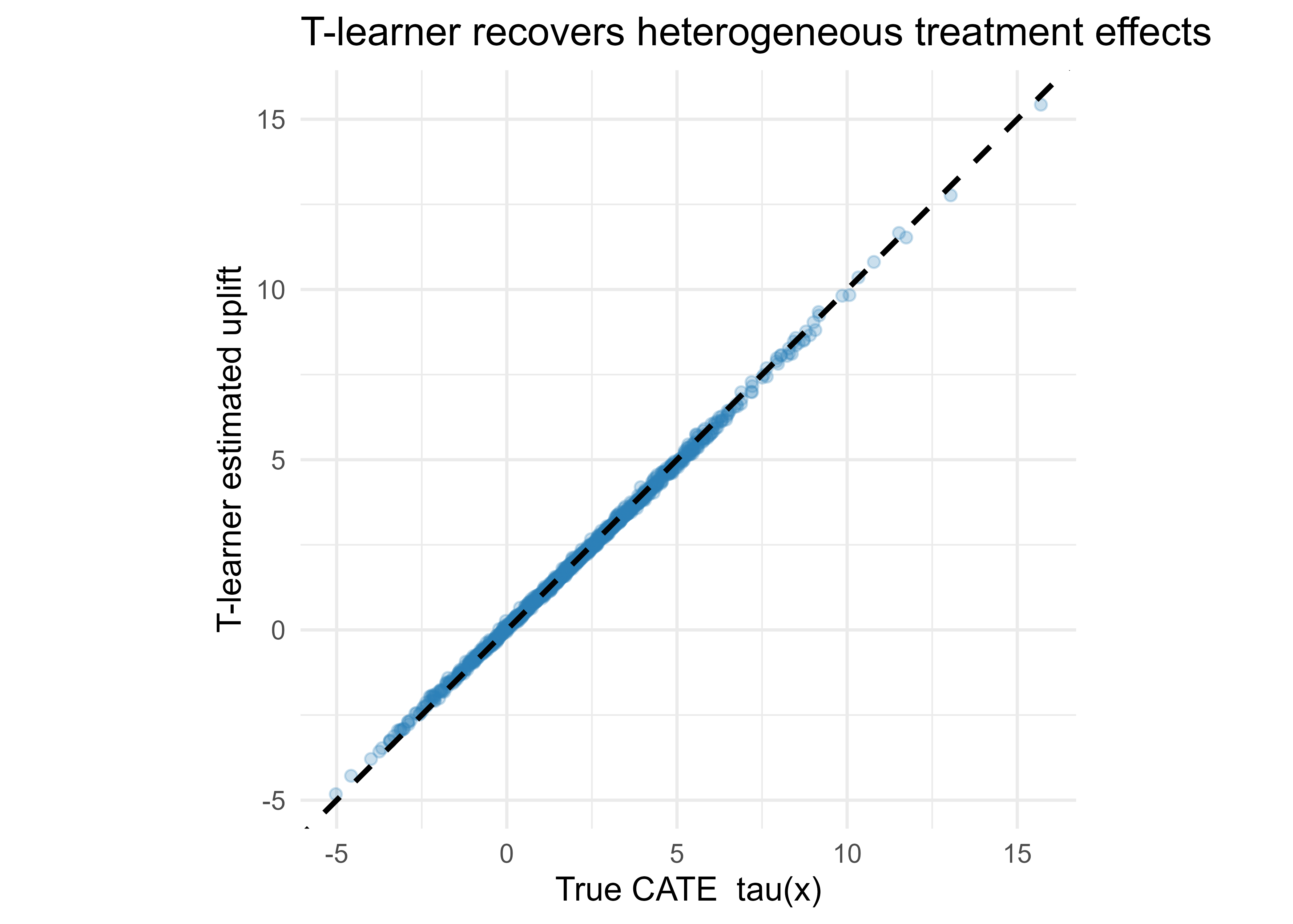
We simulate data where the true CATE is known, fit a T-learner with ordinary least squares base learners that include the right nonlinearity, and check estimated uplift against truth. Using a known data-generating process is the only way to validate a CATE method directly, because real data never reveals \(\tau_i\).
The design: outcome depends on covariates through a baseline \(b(x)\), and the treatment effect is heterogeneous, \(\tau(x) = 1 + 2\,x_1 + x_2^2\), so it varies smoothly across the feature space. Treatment is randomized with probability \(0.5\), which makes unconfoundedness hold by construction.
Tip
When you are learning or debugging a CATE method, always start on a simulation where you wrote \(\tau(x)\) yourself. It is the only setting where you can plot estimates against truth and see directly whether the method works.
Show code
.libPaths(c("C:/Users/miken/R/library-4.4", .libPaths()))set.seed(42)# ---- Data-generating process with KNOWN treatment effect ----n<-4000p<-5X<-matrix(rnorm(n*p), n, p)colnames(X)<-paste0("x", 1:p)# True CATE: heterogeneous, depends on x1 (linear) and x2 (quadratic)tau_true<-function(X)1+2*X[, 1]+X[, 2]^2# Baseline (control) response surface, nonlinear in several covariatesbaseline<-function(X)2+X[, 1]+0.5*X[, 3]-X[, 4]+sin(X[, 5])# Randomized treatment => unconfoundedness holds by designW<-rbinom(n, 1, 0.5)# Observed outcome = baseline + W * tau(X) + noisemu0<-baseline(X)mu1<-baseline(X)+tau_true(X)y<-mu0+W*tau_true(X)+rnorm(n, sd =1)dat<-data.frame(y =y, W =W, X)# ---- Train / test split ----idx_tr<-sample(seq_len(n), size =0.7*n)tr<-dat[idx_tr, ]te<-dat[-idx_tr, ]# ---- T-learner: one model per arm ----# Base learner = OLS with the quadratic term the true effect needs.form<-y~x1+x2+I(x2^2)+x3+x4+sin(x5)m1<-lm(form, data =tr[tr$W==1, ])# treated model -> mu1(x)m0<-lm(form, data =tr[tr$W==0, ])# control model -> mu0(x)# CATE estimate = difference of the two response-surface predictionstau_hat<-predict(m1, newdata =te)-predict(m0, newdata =te)# Ground-truth CATE on the test settau_te<-tau_true(as.matrix(te[, paste0("x", 1:p)]))# ---- Accuracy of the per-unit uplift estimate ----rmse<-sqrt(mean((tau_hat-tau_te)^2))bias<-mean(tau_hat-tau_te)cat(sprintf("True ATE : %.3f\n", mean(tau_te)))#> True ATE : 2.088cat(sprintf("Est. ATE : %.3f\n", mean(tau_hat)))#> Est. ATE : 2.078cat(sprintf("CATE RMSE : %.3f\n", rmse))#> CATE RMSE : 0.102cat(sprintf("CATE bias : %.3f\n", bias))#> CATE bias : -0.010library(ggplot2)ggdat<-data.frame(true =tau_te, est =tau_hat)ggplot(ggdat, aes(true, est))+geom_point(alpha =0.25, colour ="#2c7fb8")+geom_abline(slope =1, intercept =0, linetype ="dashed", linewidth =1)+labs(x ="True CATE tau(x)", y ="T-learner estimated uplift", title ="T-learner recovers heterogeneous treatment effects")+coord_equal()+theme_minimal(base_size =13)
Figure 76.1: T-learner estimated uplift versus true CATE on held-out test units. Points near the dashed 45-degree line indicate accurate per-unit effect estimates.
The estimated ATE lands near the true ATE, the per-unit RMSE is small relative to the spread of \(\tau(x)\), and the scatter in Figure 76.1 hugs the 45-degree line. The result is good here because the base learner contains the quadratic term that the true effect needs; if we used a misspecified linear base learner the quadratic part of the effect would be lost, which is the central modeling lesson: a meta-learner is only as good at capturing heterogeneity as its base learner.
76.6.1 Evaluating uplift without ground truth
Real problems give no \(\tau_i\), so we evaluate ranking quality instead. The trick is that even though we cannot check one unit’s predicted uplift against its truth, we can check whether the units the model ranks highest actually show a larger treated-minus-control gap as a group. That group-level comparison is exactly what a Qini curve measures.
The Qini curve and the related uplift curve plot cumulative incremental outcome as we treat units in descending order of predicted uplift. A model that ranks the truly responsive units first lifts off the diagonal; the area between the curve and the random-targeting line (the Qini coefficient) is the headline metric (Radcliffe (2007)). The code below sketches the computation on the held-out set using each unit’s predicted uplift to order treatment.
Note
The snippet below is a teaching simplification: it differences raw treated and control means inside each top-\(k\) slice. Production Qini implementations correct for unequal arm sizes within the slice and report the area under the curve. The shape and the intuition are the same.
Show code
.libPaths(c("C:/Users/miken/R/library-4.4", .libPaths()))# Qini-style cumulative gain on the test set, ordered by predicted uplift.ord<-order(tau_hat, decreasing =TRUE)te_ord<-te[ord, ]# Among units we "target" first, compare treated vs control mean outcomes.n_te<-nrow(te_ord)frac<-seq(0.05, 1, by =0.05)gain<-sapply(frac, function(f){k<-max(2, floor(f*n_te))top<-te_ord[seq_len(k), ]yt<-mean(top$y[top$W==1])yc<-mean(top$y[top$W==0])k*(yt-yc)# cumulative incremental outcome})qini<-data.frame(frac =frac, gain =gain)print(head(qini, 4))#> frac gain#> 1 0.05 477.7772#> 2 0.10 785.0785#> 3 0.15 1080.1164#> 4 0.20 1365.6248
In a deployment you would compare this curve across S-, T-, and X-learners and a causal forest, then pick the model with the largest area under the Qini curve, validated on data the model never saw.
76.7 Practical guidance, pitfalls, and when to use it
The methods above are only as trustworthy as the data and the validation around them. The guidance below collects the failure modes that matter most in deployment, roughly in the order you should think about them: whether to use causal ML at all, whether your data supports it, how to target, how to model, and how to keep the policy honest over time.
When to use causal ML. Reach for it whenever a decision involves acting on units rather than just sorting them: who to discount, who to call, which patients to treat, which price to show. If you only need a passive forecast, a predictive model is simpler and usually better.
Prefer randomized data when you can get it. Every method here rests on unconfoundedness. In an A/B test it holds by design and the propensity is known. With observational data you are trusting that \(X\) captures all confounders, which is an untestable assumption; spend effort on the assignment model and on overlap diagnostics.
Check overlap. If \(\hat e(x)\) is near 0 or 1 for some units, effects there are extrapolation, not estimation. Plot the propensity distribution by arm and trim or flag regions with no overlap. Inverse-propensity weights blow up exactly where overlap fails.
Do not select on the predicted score the way you would in prediction. A high outcome-prediction score does not mean high uplift. Targeting “sure things” (people who would act anyway) wastes budget; some of them may even be “sleeping dogs” whose response to contact is negative.4 Rank by estimated \(\tau(x)\), not by \(\hat\mu(x)\).
Match the base learner to the effect’s shape. As the demo shows, a meta-learner inherits its base learner’s biases. Use flexible learners (boosting, forests) unless you have strong reason to believe the effect is simple, and always validate the effect estimate, not the outcome fit.
Validate on held-out data with Qini/uplift curves or, better, a fresh randomized holdout. Outcome RMSE tells you nothing about uplift quality. Keep a randomized slice of traffic to confirm the targeting policy actually lifts the business metric.
Watch sample size in the arms. The T-learner degrades when one arm is small; switch to the X-learner or a causal forest with orthogonalization in that regime.
Beware effect drift. Treatment effects can change with seasons, competition, and audience composition faster than baseline outcomes do. Monitor the realized uplift of the deployed policy and refit on a schedule.
To summarize the chapter in one line: estimate \(\tau(x)\) with the family that matches your data (meta-learners for reuse, causal forests for inference, DML for defensible summaries), rank decisions by that estimated effect rather than by predicted outcome, and validate the ranking on held-out (ideally randomized) data with a Qini or uplift curve.
76.8 Further reading
Imbens, G. and Rubin, D. (2015). Causal Inference for Statistics, Social, and Biomedical Sciences. Cambridge University Press. (Potential outcomes, identification.)
Kunzel, S., Sekhon, J., Bickel, P., and Yu, B. (2019). “Metalearners for estimating heterogeneous treatment effects using machine learning.” PNAS. (S/T/X-learners.)
Wager, S. and Athey, S. (2018). “Estimation and inference of heterogeneous treatment effects using random forests.” JASA. (Causal forests, honesty.)
Athey, S., Tibshirani, J., and Wager, S. (2019). “Generalized random forests.” Annals of Statistics. (The grf framework.)
Chernozhukov, V. et al. (2018). “Double/debiased machine learning for treatment and structural parameters.” Econometrics Journal. (Orthogonal scores, cross-fitting.)
Nie, X. and Wager, S. (2021). “Quasi-oracle estimation of heterogeneous treatment effects.” Biometrika. (The R-learner.)
Radcliffe, N. and Surry, P. (2011). “Real-world uplift modelling with significance-based uplift trees.” (Uplift trees and Qini evaluation.)
Gutierrez, P. and Gerardy, J.-Y. (2017). “Causal inference and uplift modelling: a review of the literature.” PMLR. (Survey connecting CATE to uplift.)
Athey, Susan, Julie Tibshirani, and Stefan Wager. 2019. “Generalized Random Forests.”The Annals of Statistics 47 (2): 1148–78.
Chernozhukov, Victor, Denis Chetverikov, Mert Demirer, Esther Duflo, Christian Hansen, Whitney Newey, and James Robins. 2018. “Double/Debiased Machine Learning for Treatment and Structural Parameters.”The Econometrics Journal 21 (1): C1–68.
Kunzel, Soren R., Jasjeet S. Sekhon, Peter J. Bickel, and Bin Yu. 2019. “Metalearners for Estimating Heterogeneous Treatment Effects Using Machine Learning.”Proceedings of the National Academy of Sciences 116 (10): 4156–65.
Nie, Xinkun, and Stefan Wager. 2021. “Quasi-Oracle Estimation of Heterogeneous Treatment Effects.”Biometrika 108 (2): 299–319.
Radcliffe, Nicholas J. 2007. “Using Control Groups to Target on Predicted Lift: Building and Assessing Uplift Models.”Direct Marketing Analytics Journal, 14–21.
Wager, Stefan, and Susan Athey. 2018. “Estimation and Inference of Heterogeneous Treatment Effects Using Random Forests.”Journal of the American Statistical Association 113 (523): 1228–42.
Think of two parallel worlds for each person, one where they got the treatment and one where they did not. We only ever get to live in one of them per person, so half the data we would need is structurally missing.↩︎
The propensity \(\hat e(x)\) acts as a switch: where treated units are rare, \(\hat e(x)\) is small, so the formula leans on \(\hat\tau_1(x)\), the effect estimate imputed from the plentiful controls, and vice versa.↩︎
A nuisance is a quantity you must estimate to get at the thing you care about, but which is not itself the target. Here the response surfaces and the propensity are nuisances; the treatment effect is the target.↩︎
The uplift literature sorts people into four cells: persuadables (act only if treated, the ones you want), sure things (act either way), lost causes (never act), and sleeping dogs (treating them backfires). Only the persuadables justify spending. Outcome-prediction scores cannot tell these cells apart; CATE can.↩︎
Source Code
# Causal Machine Learning and Uplift Modeling {#sec-causal-machine-learning}```{r}#| include: falsesource("_common.R")```Most of this book asks a predictive question: given features $X$, what is the best guess for an outcome $Y$? Causal machine learning asks a different question. If we intervene and set a treatment $W$ to a particular value, how does $Y$ change, and for whom does it change the most? Predicting who will buy a product is not the same as predicting who will buy *because* we sent them a coupon. The second question is the one that drives budgets, retention campaigns, pricing, and medical decisions, and it is the one a standard supervised model does not answer on its own.This chapter connects the potential outcomes framework to the supervised learning machinery developed earlier in the book. The goal is heterogeneous treatment effect estimation: not a single average effect but a function that maps each unit's features to its own expected effect. We cover meta-learners (S-, T-, and X-learners), causal forests, and double/debiased machine learning (DML), and then turn to uplift modeling, which is the applied targeting problem that these methods solve in marketing and operations.Identification (the assumptions under which a causal effect can be recovered from observational data at all) was treated in detail in the first book of this series. Here we take identification as given and focus on estimation with flexible ML models. When the assumptions below feel unfamiliar, review the identification chapter of the first book.::: {.callout-important title="Key idea"}A predictive model ranks units by *what will happen*. A causal model ranks them by *how much your action changes what happens*. These two rankings can be almost unrelated, and confusing them is the single most common mistake in applied targeting.:::By the end of the chapter you will be able to state the estimand (the CATE) precisely, choose among the main estimator families (meta-learners, causal forests, double/debiased ML), fit a working CATE estimator in R, and evaluate it honestly when the truth is unknown.## Where this fits in a modern ML/AI workflowA typical ML workflow produces a scoring model: a churn score, a propensity score, a fraud score. Decisions then get made by thresholding that score. The hidden assumption is that the score ranks people by how much an action will help them. It usually does not. A customer with a 90% renewal probability may renew with or without a discount, so spending on them is wasted. A customer at 55% might be pushed over the line by the same discount. Causal ML estimates that *push*, the incremental effect, so that targeting spends the budget where it changes behavior.In practice causal ML sits downstream of the same feature pipelines (@sec-feature-stores), data warehouses, and experiment platforms (@sec-experiment-tracking) that feed predictive models. The natural inputs are randomized experiments (A/B tests) or logged observational data with a known or estimable assignment mechanism. The outputs feed back into the same serving and decision layers: instead of scoring "probability of conversion," you score "expected lift from the offer" and rank by that. Teams that already run experiments and have a feature store are well positioned, because the marginal cost is mostly modeling and validation, not new infrastructure.::: {.callout-tip title="When to use this"}Reach for causal ML when a decision will *act on* the units being scored (send a coupon, schedule a call, prescribe a drug, choose a price). If the action is the same for everyone and you only need a forecast to plan capacity or set a threshold, a plain predictive model is simpler and usually enough.:::## Potential outcomes recap and CATEWe use the Neyman-Rubin potential outcomes model. For each unit $i$ let $W_i \in \{0, 1\}$ be a binary treatment (1 = treated, 0 = control), let $X_i \in \mathbb{R}^p$ be pre-treatment covariates, and let $Y_i(0)$ and $Y_i(1)$ be the two potential outcomes, one for each treatment value. We observe only one of them,$$Y_i = W_i \, Y_i(1) + (1 - W_i) \, Y_i(0),$$which is the fundamental problem of causal inference: the other potential outcome is a counterfactual we never see for that unit.^[Think of two parallel worlds for each person, one where they got the treatment and one where they did not. We only ever get to live in one of them per person, so half the data we would need is structurally missing.]The unit-level treatment effect is $\tau_i = Y_i(1) - Y_i(0)$. It is not identified for a single unit because one term is always missing. What we can identify, under the assumptions below, is the Conditional Average Treatment Effect (CATE),$$\tau(x) = \mathbb{E}\!\left[\, Y_i(1) - Y_i(0) \mid X_i = x \,\right].$$Averaging $\tau(x)$ over the population gives the Average Treatment Effect (ATE), $\tau = \mathbb{E}[\tau(X)]$. CATE is the object of interest for targeting, because it tells us the effect for the subpopulation defined by $X = x$. In the uplift literature $\tau(x)$ is called the uplift or incremental effect.::: {.callout-tip title="Intuition"}We cannot measure the effect on one person, but we can compare otherwise-similar people who happened to be treated against those who were not. The CATE is the effect averaged over everyone who shares a given feature profile $x$. The finer we slice by $x$, the closer we get to a personalized effect, at the cost of noisier estimates.:::Three standard assumptions make $\tau(x)$ estimable from data. They are the same ones derived in the first book.1. Unconfoundedness (ignorability): $\{Y_i(0), Y_i(1)\} \perp W_i \mid X_i$. Treatment is as good as random once we condition on $X$. In a randomized experiment this holds by design.2. Overlap (positivity): $0 < e(x) < 1$ for all $x$, where $e(x) = \mathbb{P}(W_i = 1 \mid X_i = x)$ is the propensity score. Every type of unit has some chance of being in either arm.3. SUTVA: one unit's treatment does not affect another's outcome, and there is a single version of the treatment.Under unconfoundedness, the missing-outcome regressions are identified by the observed-data regressions. Define the response surfaces$$\mu_0(x) = \mathbb{E}[Y \mid X = x, W = 0], \qquad \mu_1(x) = \mathbb{E}[Y \mid X = x, W = 1].$$Then$$\tau(x) = \mu_1(x) - \mu_0(x),$$because conditioning on $W$ is, given $X$, the same as conditioning on the potential outcome. This single identity is the engine behind every estimator in this chapter: estimate the response surfaces (or functionals of them) with flexible ML, then difference them.To see the identity explicitly, fix $x$ and a treatment value $w$. By the definition of the observed outcome, $\mathbb{E}[Y \mid X = x, W = w] = \mathbb{E}[Y(w) \mid X = x, W = w]$, since $Y = Y(w)$ on the event $\{W = w\}$. Unconfoundedness makes $Y(w)$ independent of $W$ given $X$, so the conditioning on $W = w$ can be dropped:$$\mu_w(x) = \mathbb{E}[Y \mid X = x, W = w] = \mathbb{E}[Y(w) \mid X = x, W = w] = \mathbb{E}[Y(w) \mid X = x].$$Differencing $w = 1$ and $w = 0$ gives $\mu_1(x) - \mu_0(x) = \mathbb{E}[Y(1) - Y(0) \mid X = x] = \tau(x)$, which is the identifying identity. Overlap is what makes both conditional expectations well defined: if $e(x) = 0$ or $1$ at some $x$, one arm contributes no data there and the corresponding $\mu_w(x)$ is unidentified, so any estimate is pure extrapolation.::: {.callout-important title="Key idea"}Identification converts an impossible question (a counterfactual difference per unit) into a possible one (a difference of two ordinary regressions). Everything that follows is a different strategy for estimating those regressions, or functionals of them, accurately.:::With the estimand and the identifying identity in hand, we now turn to the estimators. The families below differ only in *how* they estimate the response surfaces and *how* they combine them.## Meta-learnersMeta-learners are recipes that turn any off-the-shelf regression learner (the "base learner") into a CATE estimator. They are attractive because you reuse the models you already trust (gradient boosting (@sec-gradient-boosting), random forests (@sec-random-forest), penalized regression) and only change how you wire them together. The names follow @kunzel2019metalearners.### S-learnerThe S-learner ("single") fits one model to the pooled data with treatment included as just another feature,$$\hat\mu(x, w) \approx \mathbb{E}[Y \mid X = x, W = w],$$and estimates $\hat\tau_S(x) = \hat\mu(x, 1) - \hat\mu(x, 0)$. To get the effect you score each unit twice, once with $w = 1$ and once with $w = 0$, and subtract. It is simple and uses all the data for one model. The risk is regularization bias toward zero: if the base learner shrinks or rarely splits on $W$ (common with tree ensembles when $W$ is one weak feature among many), the implied effect is biased small. S-learners do well when the true effect is small or smooth.::: {.callout-warning}With a tree ensemble, $W$ competes with every other feature for splits. If the effect is subtle, the trees may barely split on $W$ and the S-learner will report an effect near zero even when a real, heterogeneous effect exists.:::### T-learnerThe T-learner ("two") fits two separate models, one per arm,$$\hat\mu_0(x) \text{ on the controls}, \qquad \hat\mu_1(x) \text{ on the treated},$$and sets $\hat\tau_T(x) = \hat\mu_1(x) - \hat\mu_0(x)$. Each model can specialize to its arm, so the T-learner captures effect heterogeneity well when both arms have enough data. The weaknesses are that it splits the sample (small arms get noisy models) and that two independently regularized models can differ in ways that masquerade as treatment effect, especially when the arms have different sample sizes or covariate distributions.### X-learnerThe X-learner addresses the T-learner's imbalance problem in three steps and is the recommended default when arm sizes are very unequal (@kunzel2019metalearners). The "X" comes from the cross-step, where the model trained on one arm is used to impute the missing outcome for units in the other arm.1. Fit $\hat\mu_0$ and $\hat\mu_1$ as in the T-learner.2. Impute the individual effects by crossing the models over arms:$$\tilde D_i = Y_i - \hat\mu_0(X_i) \ \text{ for treated } i, \qquad\tilde D_i = \hat\mu_1(X_i) - Y_i \ \text{ for control } i.$$Regress $\tilde D_i$ on $X_i$ within each arm to get $\hat\tau_1(x)$ (from treated) and $\hat\tau_0(x)$ (from controls).3. Combine with a propensity weight $\hat e(x)$:$$\hat\tau_X(x) = \hat e(x)\, \hat\tau_0(x) + \bigl(1 - \hat e(x)\bigr)\, \hat\tau_1(x).$$The weighting puts more trust in the estimate built from the larger arm at each $x$, which is why the X-learner shines under imbalance.^[The propensity $\hat e(x)$ acts as a switch: where treated units are rare, $\hat e(x)$ is small, so the formula leans on $\hat\tau_1(x)$, the effect estimate imputed from the plentiful controls, and vice versa.]#### Why the cross-step works and the choice of weight {#sec-causal-machine-learning-xlearner-deriv}The cross-step is an unbiasedness argument. Take a treated unit ($W_i = 1$) and suppose $\hat\mu_0$ has converged to the truth, $\hat\mu_0 = \mu_0$. Then the imputed effect is$$\tilde D_i = Y_i - \mu_0(X_i) = Y_i(1) - \mu_0(X_i),$$and taking the conditional expectation,$$\mathbb{E}[\tilde D_i \mid X_i = x, W_i = 1]= \mathbb{E}[Y(1) \mid X = x] - \mu_0(x)= \mu_1(x) - \mu_0(x) = \tau(x),$$where the first equality uses unconfoundedness to drop the conditioning on $W_i = 1$. So regressing $\tilde D_i$ on $X_i$ over the treated units estimates $\tau(x)$, and the symmetric argument over controls (with $\hat\mu_1 = \mu_1$) gives the second estimate $\hat\tau_0(x)$. The benefit over the T-learner is that each cross-estimate uses one fitted nuisance plus the observed outcome of the *other* arm, rather than differencing two independently noisy fits.The convex combination $\hat\tau_X = g\,\hat\tau_0 + (1 - g)\,\hat\tau_1$ for a weight $g(x) \in [0, 1]$ is then chosen to minimize variance. If $\hat\tau_0$ and $\hat\tau_1$ were independent with variances $v_0(x)$ and $v_1(x)$, the variance-minimizing weight would be the inverse-variance weight $g^\star(x) = v_1(x) / (v_0(x) + v_1(x))$. Where treated units are scarce, $\hat\tau_1$ is estimated over the few treated units but relies on the control regression $\hat\mu_0$, which is accurate precisely because controls are then plentiful; @kunzel2019metalearners recommend $g(x) = \hat e(x)$ for this reason. Hence $g = \hat e$ places weight $(1 - \hat e)$ on $\hat\tau_1$ exactly when treated units are rare ($\hat e$ small), leaning on the imputation that depends on the well-estimated $\hat\mu_0$, and recovering the stated formula. Using $g \equiv 1/2$ or $g \equiv \hat e$ are both valid; the propensity weight is the default because it adapts to local imbalance.@tbl-causal-machine-learning-estimator-comparison summarizes the trade-offs. Read it as a decision aid: pick the row whose "Use when" column matches your data, then confirm with held-out evaluation.| Meta-learner | Models fit | Strength | Main failure mode | Use when ||---|---|---|---|---|| S-learner | 1 (pooled, $W$ as feature) | Data-efficient, simple | Effect biased toward zero if base learner ignores $W$ | Effect is small or smooth; treatment is a strong feature || T-learner | 2 (one per arm) | Captures heterogeneity, easy to reason about | Sample splitting; arm-specific regularization artifacts | Both arms large and roughly balanced || X-learner | 4 (two response, two effect) + propensity | Robust to unequal arm sizes | More moving parts; depends on $\hat e(x)$ | Arms imbalanced (e.g. few treated) || Causal forest | Forest of honest causal trees | Built-in CIs; targets $\tau(x)$ directly | Needs `grf`; tuning | You want valid uncertainty intervals || DML | 2 nuisances + final stage | $\sqrt n$ inference on summaries; orthogonal to nuisance error | Linear final stage limits shape | You need a defensible ATE/effect summary |: Comparison of the main CATE estimator families, with the models each fits, its primary strength, its main failure mode, and the data regime in which it is preferred. {#tbl-causal-machine-learning-estimator-comparison}## Causal forestsA causal forest (@wager2018estimation; @athey2019grf) is a random forest whose splits target treatment effect heterogeneity rather than outcome prediction. Two ideas distinguish it from a regression forest.First, splits are chosen to maximize the difference in estimated treatment effect between child nodes, so the tree carves the covariate space into regions with different $\tau(x)$. A regression forest groups units with *similar outcomes*; a causal forest groups units with *similar effects*, which is a different and harder objective. Second, honesty: the data in each tree are split into one subsample used to choose the splits and a disjoint subsample used to estimate the effect within each leaf. Honesty removes the bias that comes from using the same data to both pick a split and estimate the quantity at that split, and it is what allows valid confidence intervals.::: {.callout-tip title="Intuition"}Honesty is the statistical version of not grading your own homework. If you choose the leaf boundaries to make an effect look large and then estimate that same effect on the same rows, you will overstate it. Splitting the data in two keeps the estimate honest.:::### Splitting criterion and the forest as an adaptive kernel {#sec-causal-machine-learning-grf-deriv}Within a leaf $L$ a causal tree estimates the effect by the difference of arm means,$$\hat\tau_L = \frac{\sum_{i \in L} W_i Y_i}{\sum_{i \in L} W_i} - \frac{\sum_{i \in L} (1 - W_i) Y_i}{\sum_{i \in L} (1 - W_i)},$$which is unbiased for $\tau(x)$ on $L$ when treatment is randomized within the leaf. A regression tree chooses splits to reduce outcome variance; a causal tree instead chooses the split of parent $P$ into children $C_1, C_2$ that maximizes the heterogeneity of the effect across children. Writing $n_j = |C_j|$, the criterion is the weighted between-child effect variance$$\Delta(C_1, C_2) = \frac{n_1 n_2}{n_1 + n_2}\,\bigl(\hat\tau_{C_1} - \hat\tau_{C_2}\bigr)^2,$$which is large exactly when a split separates units with different treatment effects (the causal-tree criterion of Athey and Imbens). Maximizing $\Delta$ is equivalent to minimizing the expected squared error of the leaf effect estimates, the causal analogue of the regression tree's variance-reduction criterion. The generalized random forest of @athey2019grf replaces the raw arm-mean estimator by a locally weighted moment estimator and uses a gradient-based approximation of $\Delta$ for computational efficiency, but the principle is the same: split where the local effect changes.Honesty enforces that the sample used to choose splits (the $\mathcal{I}$ subsample) is disjoint from the sample used to fill the leaf estimates (the $\mathcal{J}$ subsample). Because the leaf value $\hat\tau_L$ is then a fixed-partition arm-mean on data independent of the partition choice, $\mathbb{E}[\hat\tau_L \mid X \in L] = \bar\tau_L$ with no optimization bias, and the within-leaf estimate is conditionally unbiased.It is useful to read the forest as an adaptive kernel. Aggregating over $B$ honest trees, the prediction at $x$ is a weighted arm-difference,$$\hat\tau(x) = \frac{\sum_i \alpha_i(x)\,W_i\,Y_i}{\sum_i \alpha_i(x)\,W_i}- \frac{\sum_i \alpha_i(x)\,(1 - W_i)\,Y_i}{\sum_i \alpha_i(x)\,(1 - W_i)} \quad\text{with}\quad\alpha_i(x) = \frac{1}{B}\sum_{b=1}^{B} \frac{\mathbf{1}\{X_i \in L_b(x)\}}{|L_b(x)|},$$where $L_b(x)$ is the leaf of tree $b$ containing $x$ and $\sum_i \alpha_i(x) = 1$. The weights $\alpha_i(x)$ are a data-adaptive, supervised kernel: they place mass on training points that repeatedly fall in the same leaves as $x$, that is, points the forest judges to have a similar treatment effect. This is the unifying view of @athey2019grf, and it connects causal forests directly to the kernel and local-regression methods of @sec-kernel.### Consistency, asymptotic normality, and the rate {#sec-causal-machine-learning-grf-theory}@wager2018estimation prove that an honest causal forest with subsampling (each tree grown on a subsample of size $s = n^\beta$, $\beta < 1$, drawn without replacement) is pointwise consistent and asymptotically Gaussian:$$\frac{\hat\tau(x) - \tau(x)}{\widehat{\mathrm{se}}(\hat\tau(x))} \xrightarrow{d} \mathcal{N}(0, 1),$$which is the basis for the reported confidence intervals. Two structural ingredients make this work. Honesty removes the optimization bias, so the estimator behaves like a U-statistic of the subsampling. The trees are also required to be *random-split* and *balanced* (each split sends at least a fraction of points to each child and each feature has a minimum split probability), which forces every coordinate of $X$ to be split and drives leaf diameter to zero, giving consistency. The variance is estimated by the infinitesimal jackknife for random forests, which `grf` returns via `estimate.variance = TRUE`.The convergence is slower than the parametric $n^{-1/2}$: the pointwise rate is $n^{-\gamma}$ with $\gamma < 1/2$ depending on the dimension $p$ and the subsample exponent $\beta$, reflecting the curse of dimensionality that all nonparametric CATE estimators face. This is the price of pointwise heterogeneity estimation, and it is exactly why DML (next section), which targets a low-dimensional summary, can attain the faster $\sqrt n$ rate for that summary.The forest produces a pointwise estimate $\hat\tau(x)$ together with an estimated standard error, so you get$$\hat\tau(x) \pm z_{1-\alpha/2}\,\widehat{\mathrm{se}}(\hat\tau(x)),$$which is rare among ML methods and valuable when a stakeholder asks "is this subgroup effect real?". Modern implementations combine the forest with the orthogonalization idea from DML (regressing out $\hat\mu(x)$ and $\hat e(x)$ first), which makes the forest robust to confounding in observational data. The `grf` package is the standard implementation; it is not installed in this environment, so the code below is shown with `eval=FALSE` but is current and runnable once you `install.packages("grf")`.::: {.callout-tip}When a stakeholder needs uncertainty ("can we be sure this segment really responds?"), the causal forest is the easiest route to honest confidence intervals on per-segment effects without hand-deriving variances.:::```{r grf-causal-forest, eval=FALSE}# Causal forest with grf (install.packages("grf"))library(grf)# X: covariate matrix, W: 0/1 treatment, Y: outcomecf <-causal_forest(X = X, Y = Y, W = W,num.trees =2000,honesty =TRUE,tune.parameters ="all")# Pointwise CATE with standard errors (honest, valid CIs)pred <-predict(cf, estimate.variance =TRUE)cate_hat <- pred$predictionsse_hat <-sqrt(pred$variance.estimates)# Doubly robust ATE and a formal test for heterogeneityaverage_treatment_effect(cf)test_calibration(cf)# Which features drive heterogeneityvariable_importance(cf)```## Double/debiased machine learningDouble/debiased ML (@chernozhukov2018dml) is the framework to reach for when you need a *summary* effect (an ATE, or a low-dimensional set of effects) with honest confidence intervals, while still using flexible ML for the nuisance pieces.^[A *nuisance* is a quantity you must estimate to get at the thing you care about, but which is not itself the target. Here the response surfaces and the propensity are nuisances; the treatment effect is the target.] The problem it solves: if you plug ML estimates of $\mu(x)$ and $e(x)$ into a naive effect formula, the slow convergence and regularization bias of the ML models leak into the effect estimate and ruin its confidence intervals.DML fixes this with two ingredients, an orthogonal score and cross-fitting.Neyman orthogonality. Instead of a moment condition that is sensitive to small errors in the nuisances, DML uses one whose derivative with respect to the nuisances is zero at the truth. For the ATE the orthogonal score is the augmented inverse-propensity (AIPW) score,$$\psi(Y, W, X; \tau, \eta) = \mu_1(x) - \mu_0(x)+ \frac{W\,(Y - \mu_1(x))}{e(x)}- \frac{(1 - W)\,(Y - \mu_0(x))}{1 - e(x)} - \tau,$$ {#eq-causal-machine-learning-aipw}with nuisances $\eta = (\mu_0, \mu_1, e)$. Because the score is orthogonal, first-order errors in $\hat\eta$ cancel, so the effect estimate is robust to moderate nuisance error. This estimator is also doubly robust: it is consistent if *either* the outcome models or the propensity model is correct.### Unbiasedness, double robustness, and the orthogonality calculation {#sec-causal-machine-learning-dml-deriv}First, the score in @eq-causal-machine-learning-aipw identifies the ATE when the nuisances are correct. Set $\eta = (\mu_0, \mu_1, e)$ at the truth and take expectations. The augmentation term has mean zero, because for the treated piece$$\mathbb{E}\!\left[\frac{W\,(Y - \mu_1(X))}{e(X)}\right]= \mathbb{E}\!\left[\frac{e(X)\,\mathbb{E}[Y - \mu_1(X) \mid X, W = 1]}{e(X)}\right] = 0,$$using the tower rule and $\mathbb{E}[Y \mid X, W = 1] = \mu_1(X)$, and symmetrically for the control piece. Hence $\mathbb{E}[\psi] = \mathbb{E}[\mu_1(X) - \mu_0(X)] - \tau = \tau_{\text{ATE}} - \tau$, so the moment $\mathbb{E}[\psi] = 0$ is solved at $\tau = \tau_{\text{ATE}}$.Double robustness. Now suppose only the propensity is correct, $\hat e = e$, but the outcome models are wrong, $\hat\mu_w \ne \mu_w$. The treated augmentation still has mean zero by the IPW identity $\mathbb{E}[W f(X)/e(X)] = \mathbb{E}[f(X)]$ applied to $f(X) = \mathbb{E}[Y \mid X, W=1] - \hat\mu_1(X)$, which cancels the bias from $\hat\mu_1$; the same holds for controls. Conversely, if the outcome models are correct, $\hat\mu_w = \mu_w$, the residuals $Y - \hat\mu_w$ have conditional mean zero and the augmentation vanishes regardless of $\hat e$, leaving $\mathbb{E}[\hat\mu_1 - \hat\mu_0] = \tau_{\text{ATE}}$. Consistency under *either* model correct is the doubly robust property.Neyman orthogonality. The key reason DML tolerates slow ML nuisance estimation is that the Gateaux (directional) derivative of the moment with respect to each nuisance vanishes at the truth. Write $m(\tau, \eta) = \mathbb{E}[\psi(\,\cdot\,; \tau, \eta)]$ and perturb the propensity in a direction $\delta(X)$, $e_t = e + t\,\delta$. Differentiating the treated augmentation term,$$\left.\frac{\partial}{\partial t} \mathbb{E}\!\left[\frac{W\,(Y - \mu_1(X))}{e(X) + t\,\delta(X)}\right]\right|_{t=0}= -\,\mathbb{E}\!\left[\frac{W\,(Y - \mu_1(X))\,\delta(X)}{e(X)^2}\right] = 0,$$because $\mathbb{E}[W(Y - \mu_1(X)) \mid X] = e(X)\cdot 0 = 0$ at the true $\mu_1$. The derivative with respect to $\mu_1$ in a direction $h(X)$ is$$\left.\frac{\partial}{\partial t}\,\mathbb{E}\!\left[(\mu_1 + t h)(X) - \frac{W\,(Y - (\mu_1 + t h)(X))}{e(X)}\cdot(-1)\right]\right|_{t=0}= \mathbb{E}\!\left[h(X)\Bigl(1 - \frac{W}{e(X)}\Bigr)\right] = 0,$$since $\mathbb{E}[W \mid X] = e(X)$. The symmetric calculation holds for $\mu_0$ and $1 - e$. All first-order nuisance derivatives are zero, so the bias from plugging in $\hat\eta$ is second order, of size $\|\hat e - e\|\cdot\|\hat\mu - \mu\|$. This product structure is what lets each nuisance converge at the slow nonparametric rate $o_p(n^{-1/4})$ while their product is $o_p(n^{-1/2})$, fast enough to be asymptotically negligible.Cross-fitting. The nuisances are estimated on one fold and the score is evaluated on a held-out fold, then rotated over $K$ folds. This breaks the dependence between the nuisance fit and the data used to estimate $\tau$, removing the overfitting bias that would otherwise remain even with an orthogonal score.Concretely, split the data into $K$ folds. For fold $k$, fit $\hat\eta^{(-k)} = (\hat\mu_0^{(-k)}, \hat\mu_1^{(-k)}, \hat e^{(-k)})$ on all *other* folds, evaluate the score $\hat\psi_i = \psi(Y_i, W_i, X_i; \tau, \hat\eta^{(-k)})$ on the held-out fold, and solve the empirical moment. Because @eq-causal-machine-learning-aipw is linear in $\tau$, the solution is the closed form$$\hat\tau_{\text{DML}} = \frac1n \sum_{k=1}^{K} \sum_{i \in I_k}\left[\hat\mu_1^{(-k)}(X_i) - \hat\mu_0^{(-k)}(X_i)+ \frac{W_i\,(Y_i - \hat\mu_1^{(-k)}(X_i))}{\hat e^{(-k)}(X_i)}- \frac{(1 - W_i)\,(Y_i - \hat\mu_0^{(-k)}(X_i))}{1 - \hat e^{(-k)}(X_i)}\right].$$ {#eq-causal-machine-learning-dml-ate}Under orthogonality, cross-fitting, and the rate condition $\|\hat e - e\|\,\|\hat\mu - \mu\| = o_p(n^{-1/2})$, this estimator satisfies $\sqrt n\,(\hat\tau_{\text{DML}} - \tau) \xrightarrow{d} \mathcal{N}(0, V)$ with $V = \mathrm{Var}(\psi(\cdot; \tau, \eta))$, and $\hat V = \frac1n \sum_i \hat\psi_i^2$ is consistent, so $\hat\tau_{\text{DML}} \pm z_{1-\alpha/2}\sqrt{\hat V / n}$ is a valid confidence interval (@chernozhukov2018dml). The estimator is $\sqrt n$-consistent and asymptotically normal even though $\hat\mu$ and $\hat e$ converge slowly. DML targets summaries by default; pairing the orthogonal score with a flexible final-stage model (R-learner, causal forest) extends it to full CATE estimation.### The R-learner {#sec-causal-machine-learning-rlearner}The R-learner (@nie2021quasi) is the orthogonalization idea applied to full CATE estimation, and it makes the connection to residual-on-residual (partialling-out) regression explicit. Start from Robinson's decomposition. Define the conditional outcome mean $m(x) = \mathbb{E}[Y \mid X = x] = \mu_0(x) + e(x)\,\tau(x)$ and the propensity $e(x)$. Writing $Y = \mu_0(X) + W\tau(X) + \varepsilon$ with $\mathbb{E}[\varepsilon \mid X, W] = 0$ and subtracting $m(X)$,$$Y - m(X) = \bigl(W - e(X)\bigr)\,\tau(X) + \varepsilon.$$ {#eq-causal-machine-learning-robinson}This is the central identity: after partialling out the marginal outcome mean and the propensity, the outcome residual equals the treatment residual times the CATE, plus noise. It motivates the R-learner objective, which estimates $\tau$ by a weighted least-squares fit of outcome residuals on treatment residuals,$$\hat\tau = \arg\min_{\tau}\ \frac1n \sum_{i=1}^{n}\Bigl[\bigl(Y_i - \hat m^{(-k(i))}(X_i)\bigr) - \bigl(W_i - \hat e^{(-k(i))}(X_i)\bigr)\,\tau(X_i)\Bigr]^2 + \Lambda(\tau),$$ {#eq-causal-machine-learning-rloss}where $\hat m$ and $\hat e$ are cross-fitted nuisances, $\Lambda$ is a regularizer (a penalty, a kernel bandwidth, or the implicit regularization of a chosen function class), and $k(i)$ denotes the fold of unit $i$. The loss in @eq-causal-machine-learning-rloss is the empirical R-loss; its population minimizer is the true $\tau(x)$ by @eq-causal-machine-learning-robinson, since the residual $W - e(X)$ has conditional mean zero so the cross term with $\varepsilon$ integrates out.For a constant $\tau$ and no penalty, minimizing @eq-causal-machine-learning-rloss is an ordinary least squares regression of $\tilde Y = Y - \hat m$ on $\tilde W = W - \hat e$ through the origin, giving the closed form$$\hat\tau = \frac{\sum_i \tilde W_i\,\tilde Y_i}{\sum_i \tilde W_i^{\,2}},$$the classical partialling-out estimator. For a flexible $\tau(\cdot)$, @eq-causal-machine-learning-rloss is a weighted regression problem with weights $(W_i - \hat e_i)^2$ and pseudo-outcome $(Y_i - \hat m_i)/(W_i - \hat e_i)$, so any squared-error learner (lasso, boosting, neural net) can be the final stage. @nie2021quasi prove a quasi-oracle bound: the R-learner's CATE estimate converges at the rate it would achieve if the nuisances were known exactly, provided the nuisance product error is $o_p(n^{-1/2})$, the same orthogonality dividend seen for the ATE.::: {.callout-tip title="Intuition"}Orthogonality makes the effect estimate insensitive to small errors in the nuisance models (the gradient in their direction is zero at the truth), and cross-fitting makes sure those nuisance models were never fit on the rows used to score them. Together they let you use heavy ML for the hard parts while keeping clean inference for the part you report.:::## Runnable demo: T-learner CATE on simulated dataWe simulate data where the true CATE is known, fit a T-learner with ordinary least squares base learners that include the right nonlinearity, and check estimated uplift against truth. Using a known data-generating process is the only way to validate a CATE method directly, because real data never reveals $\tau_i$.The design: outcome depends on covariates through a baseline $b(x)$, and the treatment effect is heterogeneous, $\tau(x) = 1 + 2\,x_1 + x_2^2$, so it varies smoothly across the feature space. Treatment is randomized with probability $0.5$, which makes unconfoundedness hold by construction.::: {.callout-tip}When you are learning or debugging a CATE method, always start on a simulation where you wrote $\tau(x)$ yourself. It is the only setting where you can plot estimates against truth and see directly whether the method works.:::```{r fig-causal-machine-learning-tlearner-scatter, eval=TRUE, message=FALSE, warning=FALSE, fig.width=7, fig.height=5, fig.cap="T-learner estimated uplift versus true CATE on held-out test units. Points near the dashed 45-degree line indicate accurate per-unit effect estimates."}.libPaths(c("C:/Users/miken/R/library-4.4", .libPaths()))set.seed(42)# ---- Data-generating process with KNOWN treatment effect ----n <-4000p <-5X <-matrix(rnorm(n * p), n, p)colnames(X) <-paste0("x", 1:p)# True CATE: heterogeneous, depends on x1 (linear) and x2 (quadratic)tau_true <-function(X) 1+2* X[, 1] + X[, 2]^2# Baseline (control) response surface, nonlinear in several covariatesbaseline <-function(X) 2+ X[, 1] +0.5* X[, 3] - X[, 4] +sin(X[, 5])# Randomized treatment => unconfoundedness holds by designW <-rbinom(n, 1, 0.5)# Observed outcome = baseline + W * tau(X) + noisemu0 <-baseline(X)mu1 <-baseline(X) +tau_true(X)y <- mu0 + W *tau_true(X) +rnorm(n, sd =1)dat <-data.frame(y = y, W = W, X)# ---- Train / test split ----idx_tr <-sample(seq_len(n), size =0.7* n)tr <- dat[idx_tr, ]te <- dat[-idx_tr, ]# ---- T-learner: one model per arm ----# Base learner = OLS with the quadratic term the true effect needs.form <- y ~ x1 + x2 +I(x2^2) + x3 + x4 +sin(x5)m1 <-lm(form, data = tr[tr$W ==1, ]) # treated model -> mu1(x)m0 <-lm(form, data = tr[tr$W ==0, ]) # control model -> mu0(x)# CATE estimate = difference of the two response-surface predictionstau_hat <-predict(m1, newdata = te) -predict(m0, newdata = te)# Ground-truth CATE on the test settau_te <-tau_true(as.matrix(te[, paste0("x", 1:p)]))# ---- Accuracy of the per-unit uplift estimate ----rmse <-sqrt(mean((tau_hat - tau_te)^2))bias <-mean(tau_hat - tau_te)cat(sprintf("True ATE : %.3f\n", mean(tau_te)))cat(sprintf("Est. ATE : %.3f\n", mean(tau_hat)))cat(sprintf("CATE RMSE : %.3f\n", rmse))cat(sprintf("CATE bias : %.3f\n", bias))library(ggplot2)ggdat <-data.frame(true = tau_te, est = tau_hat)ggplot(ggdat, aes(true, est)) +geom_point(alpha =0.25, colour ="#2c7fb8") +geom_abline(slope =1, intercept =0, linetype ="dashed", linewidth =1) +labs(x ="True CATE tau(x)", y ="T-learner estimated uplift",title ="T-learner recovers heterogeneous treatment effects") +coord_equal() +theme_minimal(base_size =13)```The estimated ATE lands near the true ATE, the per-unit RMSE is small relative to the spread of $\tau(x)$, and the scatter in @fig-causal-machine-learning-tlearner-scatter hugs the 45-degree line. The result is good here because the base learner contains the quadratic term that the true effect needs; if we used a misspecified linear base learner the quadratic part of the effect would be lost, which is the central modeling lesson: a meta-learner is only as good at capturing heterogeneity as its base learner.### Evaluating uplift without ground truthReal problems give no $\tau_i$, so we evaluate ranking quality instead. The trick is that even though we cannot check one unit's predicted uplift against its truth, we *can* check whether the units the model ranks highest actually show a larger treated-minus-control gap as a group. That group-level comparison is exactly what a Qini curve measures.The Qini curve and the related uplift curve plot cumulative incremental outcome as we treat units in descending order of predicted uplift. A model that ranks the truly responsive units first lifts off the diagonal; the area between the curve and the random-targeting line (the Qini coefficient) is the headline metric (@radcliffe2007uplift). The code below sketches the computation on the held-out set using each unit's predicted uplift to order treatment.::: {.callout-note}The snippet below is a teaching simplification: it differences raw treated and control means inside each top-$k$ slice. Production Qini implementations correct for unequal arm sizes within the slice and report the area under the curve. The shape and the intuition are the same.:::```{r qini-sketch, eval=TRUE, message=FALSE, warning=FALSE}.libPaths(c("C:/Users/miken/R/library-4.4", .libPaths()))# Qini-style cumulative gain on the test set, ordered by predicted uplift.ord <-order(tau_hat, decreasing =TRUE)te_ord <- te[ord, ]# Among units we "target" first, compare treated vs control mean outcomes.n_te <-nrow(te_ord)frac <-seq(0.05, 1, by =0.05)gain <-sapply(frac, function(f) { k <-max(2, floor(f * n_te)) top <- te_ord[seq_len(k), ] yt <-mean(top$y[top$W ==1]) yc <-mean(top$y[top$W ==0]) k * (yt - yc) # cumulative incremental outcome})qini <-data.frame(frac = frac, gain = gain)print(head(qini, 4))```In a deployment you would compare this curve across S-, T-, and X-learners and a causal forest, then pick the model with the largest area under the Qini curve, validated on data the model never saw.## Practical guidance, pitfalls, and when to use itThe methods above are only as trustworthy as the data and the validation around them. The guidance below collects the failure modes that matter most in deployment, roughly in the order you should think about them: whether to use causal ML at all, whether your data supports it, how to target, how to model, and how to keep the policy honest over time.When to use causal ML. Reach for it whenever a decision involves *acting on* units rather than just sorting them: who to discount, who to call, which patients to treat, which price to show. If you only need a passive forecast, a predictive model is simpler and usually better.Prefer randomized data when you can get it. Every method here rests on unconfoundedness. In an A/B test it holds by design and the propensity is known. With observational data you are trusting that $X$ captures all confounders, which is an untestable assumption; spend effort on the assignment model and on overlap diagnostics.Check overlap. If $\hat e(x)$ is near 0 or 1 for some units, effects there are extrapolation, not estimation. Plot the propensity distribution by arm and trim or flag regions with no overlap. Inverse-propensity weights blow up exactly where overlap fails.Do not select on the predicted score the way you would in prediction. A high outcome-prediction score does not mean high uplift. Targeting "sure things" (people who would act anyway) wastes budget; some of them may even be "sleeping dogs" whose response to contact is negative.^[The uplift literature sorts people into four cells: *persuadables* (act only if treated, the ones you want), *sure things* (act either way), *lost causes* (never act), and *sleeping dogs* (treating them backfires). Only the persuadables justify spending. Outcome-prediction scores cannot tell these cells apart; CATE can.] Rank by estimated $\tau(x)$, not by $\hat\mu(x)$.Match the base learner to the effect's shape. As the demo shows, a meta-learner inherits its base learner's biases. Use flexible learners (boosting, forests) unless you have strong reason to believe the effect is simple, and always validate the *effect* estimate, not the outcome fit.Validate on held-out data with Qini/uplift curves or, better, a fresh randomized holdout. Outcome RMSE tells you nothing about uplift quality. Keep a randomized slice of traffic to confirm the targeting policy actually lifts the business metric.Watch sample size in the arms. The T-learner degrades when one arm is small; switch to the X-learner or a causal forest with orthogonalization in that regime.Beware effect drift. Treatment effects can change with seasons, competition, and audience composition faster than baseline outcomes do. Monitor the realized uplift of the deployed policy and refit on a schedule.To summarize the chapter in one line: estimate $\tau(x)$ with the family that matches your data (meta-learners for reuse, causal forests for inference, DML for defensible summaries), rank decisions by that estimated effect rather than by predicted outcome, and validate the ranking on held-out (ideally randomized) data with a Qini or uplift curve.## Further reading- Imbens, G. and Rubin, D. (2015). *Causal Inference for Statistics, Social, and Biomedical Sciences*. Cambridge University Press. (Potential outcomes, identification.)- Kunzel, S., Sekhon, J., Bickel, P., and Yu, B. (2019). "Metalearners for estimating heterogeneous treatment effects using machine learning." *PNAS*. (S/T/X-learners.)- Wager, S. and Athey, S. (2018). "Estimation and inference of heterogeneous treatment effects using random forests." *JASA*. (Causal forests, honesty.)- Athey, S., Tibshirani, J., and Wager, S. (2019). "Generalized random forests." *Annals of Statistics*. (The `grf` framework.)- Chernozhukov, V. et al. (2018). "Double/debiased machine learning for treatment and structural parameters." *Econometrics Journal*. (Orthogonal scores, cross-fitting.)- Nie, X. and Wager, S. (2021). "Quasi-oracle estimation of heterogeneous treatment effects." *Biometrika*. (The R-learner.)- Radcliffe, N. and Surry, P. (2011). "Real-world uplift modelling with significance-based uplift trees." (Uplift trees and Qini evaluation.)- Gutierrez, P. and Gerardy, J.-Y. (2017). "Causal inference and uplift modelling: a review of the literature." *PMLR*. (Survey connecting CATE to uplift.)