34 Topic Models and Latent Dirichlet Allocation
A large collection of documents is hard to read. A corpus of ten thousand news articles, scientific abstracts, or customer reviews contains far more text than any person can absorb, yet we often suspect that it is organized around a small number of recurring themes. Some articles are about sports, some about finance, some about politics, and many mix two or three of these in varying proportions. Topic modeling is the unsupervised attempt to recover those themes automatically, using nothing but the words on the page and no labels at all.
The plain-language idea is this. Imagine each theme, which we will call a topic, as a characteristic vocabulary: a “finance” topic uses words like market, rate, and profit frequently, while a “sports” topic favors team, game, and score. A document is then a blend of a few topics, and the words we actually observe are drawn from the vocabularies of whichever topics that document blends. Topic modeling inverts this story. Given only the observed words, it estimates both the topic vocabularies (shared across the whole corpus) and the per-document blend (specific to each document). The most widely used model of this kind is Latent Dirichlet Allocation (LDA), introduced by Blei, Ng, and Jordan (2003), and it is the focus of this chapter.
LDA sits at an intersection of several ideas elsewhere in this book. It is a soft clustering of documents, so it is a cousin of the mixture models in Chapter 23; it is a low-rank factorization of a word-count matrix, so it is closely related to the matrix factorizations in Chapter 27; and it is a fully generative probabilistic model, fit by the same variational and sampling machinery used throughout Chapter 32. Understanding LDA well therefore reinforces three threads at once.
Key idea
LDA treats every document as a mixture over a fixed set of latent topics, and every topic as a distribution over the vocabulary. Words are the only observed quantity. Both the per-document mixture and the per-topic vocabulary are inferred jointly, so the model discovers structure that no one labeled in advance.
34.1 The bag-of-words and document-term setup
Before any modeling, text must be turned into numbers. Topic models use the simplest useful representation, the bag of words: each document is reduced to the counts of each vocabulary word it contains, discarding word order entirely. The phrase “the cat sat” and “sat the cat” become the same bag. This is a strong simplification, but it is exactly the assumption that makes the model tractable and, empirically, it captures thematic content surprisingly well.
Fix a vocabulary of \(V\) distinct word types, indexed \(1, \dots, V\). A corpus has \(D\) documents. Document \(d\) has \(N_d\) word tokens (occurrences), written \(w_d = (w_{d1}, \dots, w_{d N_d})\), where each token \(w_{dn} \in \{1, \dots, V\}\) names a vocabulary entry. Collecting counts across the corpus gives the \(D \times V\) document-term matrix \(\mathbf{C}\), where \(C_{dv}\) is the number of times word \(v\) appears in document \(d\). This matrix is typically very sparse, since any one document uses only a small fraction of the vocabulary.
Exchangeability
The bag-of-words assumption is formally an assumption of exchangeability: the words in a document are treated as exchangeable, meaning their joint distribution is invariant to permutation. By de Finetti’s theorem, an infinitely exchangeable sequence can be written as a mixture of independent and identically distributed draws conditional on a latent parameter. LDA’s per-document topic mixture is exactly that latent parameter, which is why the bag-of-words view and the mixture view are two sides of one coin.
34.2 The LDA generative story
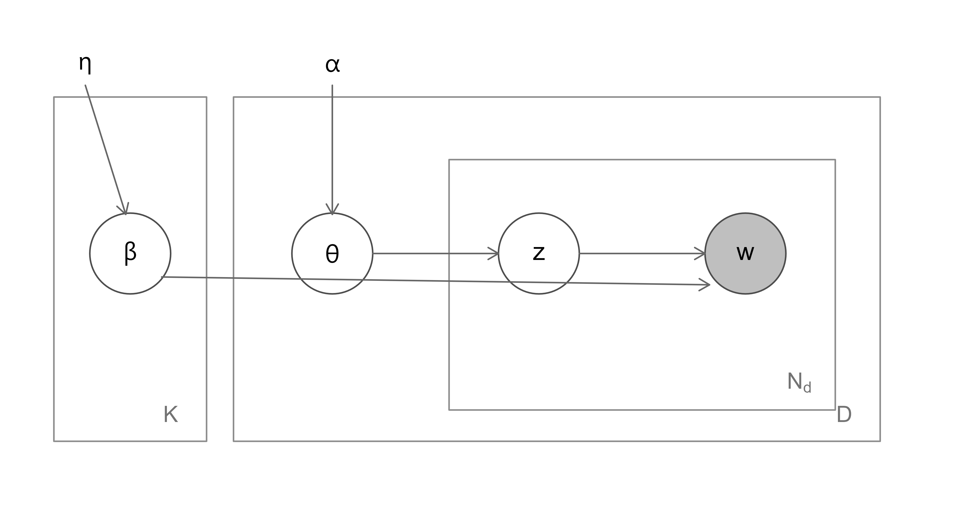
LDA is defined by a generative process: a recipe that, run forward, would produce a corpus. We then run it backward to infer the hidden quantities. Fix the number of topics \(K\) and two concentration hyperparameters, \(\alpha\) (a \(K\)-vector or scalar) and \(\eta\) (a \(V\)-vector or scalar).
First, draw the \(K\) topics. Each topic \(k\) is a distribution \(\beta_k\) over the \(V\) words, drawn from a Dirichlet prior, \[ \beta_k \sim \operatorname{Dirichlet}(\eta), \qquad k = 1, \dots, K . \tag{34.1}\] Each \(\beta_k\) is a point on the \(V\)-dimensional simplex, so \(\beta_{kv} \ge 0\) and \(\sum_v \beta_{kv} = 1\); the entry \(\beta_{kv}\) is the probability that topic \(k\) emits word \(v\).
Then, for each document \(d\), draw its topic proportions and its words:
- Draw the per-document topic mixture \(\theta_d \sim \operatorname{Dirichlet}(\alpha)\), a point on the \(K\)-simplex.
- For each token position \(n = 1, \dots, N_d\):
- Draw a topic assignment \(z_{dn} \sim \operatorname{Categorical}(\theta_d)\), with \(z_{dn} \in \{1, \dots, K\}\).
- Draw the observed word \(w_{dn} \sim \operatorname{Categorical}(\beta_{z_{dn}})\).
The latent variables are the topics \(\beta = \{\beta_k\}\), the document mixtures \(\theta = \{\theta_d\}\), and the per-token assignments \(z = \{z_{dn}\}\). Only \(w\) is observed. Figure 34.1 shows the dependency structure in plate notation.
34.2.1 The joint distribution
Multiplying the conditional pieces in the generative story gives the joint distribution of everything, observed and latent. For a single document \(d\), \[ p(\theta_d, z_d, w_d \mid \alpha, \beta) = p(\theta_d \mid \alpha) \prod_{n=1}^{N_d} p(z_{dn} \mid \theta_d)\, p(w_{dn} \mid z_{dn}, \beta) . \tag{34.2}\] Across the corpus, including the topic prior, the full joint is \[ p(w, z, \theta, \beta \mid \alpha, \eta) = \prod_{k=1}^{K} p(\beta_k \mid \eta) \prod_{d=1}^{D} p(\theta_d \mid \alpha) \prod_{n=1}^{N_d} p(z_{dn} \mid \theta_d)\, p(w_{dn} \mid \beta_{z_{dn}}) . \tag{34.3}\] The Dirichlet density that appears here is \[ p(\theta_d \mid \alpha) = \frac{\Gamma\!\left(\sum_{k} \alpha_k\right)}{\prod_{k} \Gamma(\alpha_k)} \prod_{k=1}^{K} \theta_{dk}^{\alpha_k - 1} , \tag{34.4}\] and the analogous form holds for \(p(\beta_k \mid \eta)\). The marginal likelihood of the observed corpus integrates out all latent variables, \[ p(w \mid \alpha, \eta) = \int \!\! \int \sum_{z}\, p(w, z, \theta, \beta \mid \alpha, \eta)\; d\theta\, d\beta , \tag{34.5}\] and this integral is intractable: the sum over \(z\) has \(K^{\,\sum_d N_d}\) terms and is coupled to \(\theta\) and \(\beta\) through the integrals. The entire inference problem is the problem of approximating Equation 34.5 and the posterior \(p(z, \theta, \beta \mid w)\) it normalizes.
Why Dirichlet?
The Dirichlet is the conjugate prior of the categorical and multinomial distributions. Conjugacy means the posterior stays in the same family, so adding observed counts to a Dirichlet just adds to its parameters. This is what makes the collapsed sampler below have such a clean closed form, and it is the same conjugacy that powers Bayesian updating elsewhere in Chapter 32. A small concentration (\(\alpha_k < 1\)) favors sparse mixtures, where each document uses only a few topics, which is usually what we want.
34.3 Inference
We cannot compute the posterior exactly, so we approximate it. Two approaches dominate: collapsed Gibbs sampling, which draws samples from the posterior, and variational EM, which fits the best tractable surrogate. We sketch both and state the update equations without grinding through every line of algebra.
34.3.1 Collapsed Gibbs sampling
The key trick is to collapse (integrate out) the continuous variables \(\theta\) and \(\beta\) analytically, using Dirichlet-multinomial conjugacy, leaving a posterior only over the discrete assignments \(z\). Because of conjugacy, \(\int p(w, z, \theta, \beta) \, d\theta\, d\beta\) has a closed form in terms of word and topic counts, and the conditional distribution of a single assignment given all others becomes a simple product of two ratios.
Let \(n_{dk}^{\neg dn}\) be the number of tokens in document \(d\) currently assigned to topic \(k\), excluding the token at position \(n\), and let \(m_{kv}^{\neg dn}\) be the number of times word \(v\) is assigned to topic \(k\) across the corpus, again excluding the current token. Write \(w_{dn} = v\). The collapsed Gibbs update is \[ p\!\left(z_{dn} = k \mid z^{\neg dn}, w\right) \;\propto\; \bigl(n_{dk}^{\neg dn} + \alpha_k\bigr)\, \frac{m_{kv}^{\neg dn} + \eta_v}{\sum_{v'=1}^{V} \bigl(m_{kv'}^{\neg dn} + \eta_{v'}\bigr)} . \tag{34.6}\] The first factor is the document’s current preference for topic \(k\) (smoothed by \(\alpha\)); the second factor is topic \(k\)’s current preference for word \(v\) (smoothed by \(\eta\)). We sweep through every token repeatedly, resampling each \(z_{dn}\) from Equation 34.6, and after a burn-in the counts stabilize. Point estimates of the topics and mixtures recover by plugging the final counts back into the posterior means, \[ \hat\beta_{kv} = \frac{m_{kv} + \eta_v}{\sum_{v'} (m_{kv'} + \eta_{v'})}, \qquad \hat\theta_{dk} = \frac{n_{dk} + \alpha_k}{\sum_{k'} (n_{dk'} + \alpha_{k'})} . \tag{34.7}\] This sampler, due to Griffiths and Steyvers (2004), is easy to implement and is what we code from scratch below.
34.3.2 Variational EM
The alternative posits a factorized surrogate \(q\) and minimizes its Kullback-Leibler divergence to the true posterior, equivalently maximizing the evidence lower bound (ELBO). LDA’s mean-field family fully factorizes the latent variables, \[ q(z, \theta, \beta) = \prod_{k} q(\beta_k \mid \lambda_k) \prod_{d} q(\theta_d \mid \gamma_d) \prod_{n} q(z_{dn} \mid \phi_{dn}) , \tag{34.8}\] with \(q(\theta_d)\) and \(q(\beta_k)\) Dirichlet (parameters \(\gamma_d\), \(\lambda_k\)) and \(q(z_{dn})\) categorical (parameter \(\phi_{dn}\)). Maximizing the ELBO gives coordinate-ascent updates that alternate an E-step over per-document variables and an M-step over topics. The E-step updates, for each document, are \[ \phi_{dnk} \;\propto\; \beta_{k, w_{dn}}\, \exp\!\bigl(\psi(\gamma_{dk})\bigr), \qquad \gamma_{dk} = \alpha_k + \sum_{n=1}^{N_d} \phi_{dnk} , \tag{34.9}\] where \(\psi\) is the digamma function, iterated to convergence per document. The M-step aggregates the responsibilities into the topics, \[ \lambda_{kv} = \eta_v + \sum_{d=1}^{D} \sum_{n=1}^{N_d} \phi_{dnk}\, \mathbb{1}\{w_{dn} = v\} . \tag{34.10}\] This is structurally the same expectation-maximization loop used for Gaussian mixtures in Chapter 32: \(\phi\) plays the role of soft responsibilities, the \(\gamma\)/\(\lambda\) updates are the weighted-count M-step. The original variational treatment is Blei, Ng, and Jordan (2003); the online stochastic version of Hoffman, Blei, and Bach (2010) is what scales LDA to millions of documents and is the default in most libraries.
Sampling versus variational, which to use
Collapsed Gibbs is unbiased in the limit of infinite samples and is simple to code, but mixing can be slow and convergence is hard to diagnose. Variational EM is deterministic, fast, and easy to monitor through the ELBO, but it is biased: mean-field factorization understates posterior uncertainty and can settle in poor local optima. For small corpora and pedagogy, use Gibbs; for production-scale fitting, use (online) variational inference.
34.4 Evaluation: perplexity and coherence
Two questions matter when judging a fitted model: does it predict held-out text well, and are its topics interpretable to a human? The two questions, perhaps surprisingly, do not always agree.
Perplexity measures predictive fit. On a held-out set of documents \(w^{\text{test}}\), it is the exponentiated per-word negative log-likelihood, \[ \operatorname{perplexity}(w^{\text{test}}) = \exp\!\left( - \frac{\sum_{d} \log p(w_d^{\text{test}})}{\sum_{d} N_d} \right) , \tag{34.11}\] where lower is better. Perplexity is a monotone transform of held-out log-likelihood, so it is the natural way to choose \(K\) by cross-validation: fit several values of \(K\), evaluate held-out perplexity, and pick the elbow. The catch, documented by Chang et al. (2009), is that perplexity often keeps improving as \(K\) grows past the point where humans find the topics meaningful.
Topic coherence targets interpretability directly. The UMass coherence of a topic, using its top \(M\) words ranked by \(\beta_{kv}\), is \[ C_{\text{UMass}}(k) = \sum_{i=2}^{M} \sum_{j=1}^{i-1} \log \frac{D(w_i, w_j) + \varepsilon}{D(w_j)} , \tag{34.12}\] where \(D(w_j)\) is the number of documents containing word \(w_j\), \(D(w_i, w_j)\) the number containing both, and \(\varepsilon\) a small smoothing constant. High coherence means the top words of a topic genuinely co-occur, which correlates with human judgments far better than perplexity does. In practice, report both and let coherence guard against the over-fragmentation that perplexity invites.
34.5 Relation to NMF and pLSA
LDA did not appear from nowhere; it is the Bayesian endpoint of a short lineage of matrix-factorization models, and seeing the connection demystifies it.
Probabilistic Latent Semantic Analysis (pLSA), due to Hofmann (1999), uses the same emission structure but treats \(\theta_d\) as a free parameter per document rather than a draw from a prior. Its word probability is \[ p(w = v \mid d) = \sum_{k=1}^{K} \theta_{dk}\, \beta_{kv} , \tag{34.13}\] fit by maximum likelihood with EM. LDA is exactly pLSA with a Dirichlet prior placed on \(\theta_d\) (and optionally on \(\beta_k\)). The prior is not cosmetic: pLSA has a \(\theta_d\) for every training document and therefore no principled way to assign topics to a new, unseen document, and its parameter count grows with the corpus so it overfits. The Dirichlet prior in LDA fixes both problems by making \(\theta_d\) a latent variable to be integrated out rather than a parameter to be fit.
Non-negative matrix factorization (NMF), discussed in Chapter 27, factors the document-term matrix as \(\mathbf{C} \approx \mathbf{W}\mathbf{H}\) with \(\mathbf{W} \ge 0\) (\(D \times K\)) and \(\mathbf{H} \ge 0\) (\(K \times V\)). Rows of \(\mathbf{W}\) act like document-topic weights and rows of \(\mathbf{H}\) like topic-word weights, exactly mirroring \(\theta\) and \(\beta\). The precise correspondence is in the loss: minimizing the generalized Kullback-Leibler divergence between \(\mathbf{C}\) and \(\mathbf{W}\mathbf{H}\) is equivalent to maximizing the pLSA likelihood Equation 34.13, so NMF with KL loss is pLSA up to normalization. LDA adds the Dirichlet prior and the resulting Bayesian averaging that NMF lacks.
One picture
All three methods factor a word-count matrix into a documents-by-topics part and a topics-by-words part. NMF does it as deterministic non-negative least-divergence; pLSA does it as maximum-likelihood under a multinomial; LDA does it as full Bayesian inference with Dirichlet priors. Reading them as one family is the fastest way to remember what each adds.
34.6 Assumptions, properties, and failure modes
LDA buys tractability with assumptions, and knowing them tells you when it will disappoint.
The bag-of-words assumption discards word order, so LDA cannot distinguish “dog bites man” from “man bites dog” and learns nothing about syntax or phrases unless you pre-tokenize n-grams. The number of topics \(K\) is fixed in advance and must be chosen by perplexity, coherence, or a nonparametric extension (the hierarchical Dirichlet process learns \(K\) from data). The model assumes topics are uncorrelated through the Dirichlet, which is unrealistic since a “finance” topic and an “economics” topic tend to co-occur; the correlated topic model replaces the Dirichlet with a logistic-normal prior to fix this. The topics themselves are exchangeable, so the labeling is arbitrary and not identifiable across runs, which complicates comparison.
On complexity, collapsed Gibbs costs \(O(K)\) per token per sweep, hence \(O(K \sum_d N_d)\) per full pass, with memory dominated by the sparse counts. Variational EM has the same per-iteration order but converges in far fewer passes and parallelizes cleanly. Both degrade when the vocabulary is huge or documents are very short (tweets), because short documents give little evidence for their mixture. Stop-word removal and pruning rare terms matter a great deal in practice: leaving common function words in produces an uninformative “the/of/and” topic that absorbs probability mass.
Common pitfalls
Three failures recur. First, forgetting to remove stop words yields a junk topic of function words. Second, setting \(K\) too high fragments coherent themes into near-duplicates that perplexity rewards but humans reject. Third, comparing topic labels across two fits as if topic 3 means the same thing in both: topics are unidentifiable up to permutation and must be aligned (for example by matching \(\beta\) vectors) before comparison.
34.7 Practical workflow
A reliable recipe. Build the document-term matrix after lower-casing, removing stop words and punctuation, and optionally stemming or lemmatizing; prune terms that appear in too few or nearly all documents. Choose a small grid of \(K\) values and fit each, holding out a fraction of each document’s tokens to compute perplexity Equation 34.11, and compute coherence Equation 34.12 on the rest. Pick \(K\) where coherence peaks and perplexity has stopped improving sharply. Set \(\alpha\) small (often \(50/K\) or \(0.1\)) to encourage sparse document mixtures and \(\eta\) small (often \(0.01\)) for sparse topics. Inspect the top words per topic, assign human-readable labels, and validate by reading a few high-probability documents per topic. Only then use \(\theta\) as a feature representation for downstream tasks, where it behaves as a learned low-dimensional embedding much like the codes from an autoencoder (Chapter 41) or the document vectors discussed alongside transformers (Chapter 38).
In R, the standard library is topicmodels, which wraps both the variational EM fit (method = "VEM") and the collapsed Gibbs sampler (method = "Gibbs"), built on tm/slam document-term matrices. The following shows the typical call. It is not executed here because topicmodels is not part of the runnable environment for this build, but it is the canonical usage.
Show code
library(tm)
library(topicmodels)

# `corpus_text` is a character vector, one string per document
corpus <- VCorpus(VectorSource(corpus_text))
corpus <- tm_map(corpus, content_transformer(tolower))
corpus <- tm_map(corpus, removePunctuation)
corpus <- tm_map(corpus, removeWords, stopwords("en"))
dtm    <- DocumentTermMatrix(corpus)
dtm    <- removeSparseTerms(dtm, 0.99)

# Fit LDA with K = 4 topics via collapsed Gibbs sampling
set.seed(1)
fit <- LDA(dtm, k = 4, method = "Gibbs",
           control = list(iter = 2000, burnin = 500, seed = 1))

terms(fit, 8)              # top 8 words per topic (the beta matrix)
posterior(fit)$topics     # document-topic matrix (theta)
perplexity(fit, dtm)      # held-out perplexity
34.8 A runnable demonstration in base R
To make every moving part visible we build a tiny synthetic corpus from two known topics, form the document-term matrix by hand, fit LDA with a collapsed Gibbs sampler written from scratch using Equation 34.6, and finally show the fixed-point reconstruction of the topic-word and document-topic matrices via Equation 34.7. Everything uses base R only.
34.8.1 Building the document-term matrix
We define two ground-truth topics over a six-word vocabulary, one “weather” topic and one “finance” topic, then generate documents by sampling words from a per-document blend of the two.
Show code
set.seed(42)

vocab <- c("rain", "sun", "cloud", "stock", "bond", "yield")
V <- length(vocab); K <- 2

# True topic-word distributions (rows = topics, sum to 1)
beta_true <- rbind(
  weather = c(rain = .34, sun = .33, cloud = .30, stock = .01, bond = .01, yield = .01),
  finance = c(rain = .01, sun = .01, cloud = .01, stock = .34, bond = .33, yield = .30)
)

D  <- 30                       # documents
Nd <- 40                       # tokens per document
w_share <- sort(runif(D))      # each doc's true weather share (sorted for the plot)

# Generate token counts: for each token pick a topic by theta, then a word by beta
make_doc <- function(share) {
  topics <- sample(1:2, Nd, replace = TRUE, prob = c(share, 1 - share))
  words  <- vapply(topics, function(k) sample(1:V, 1, prob = beta_true[k, ]), integer(1))
  tabulate(words, nbins = V)
}
C <- t(vapply(w_share, make_doc, integer(V)))   # D x V document-term matrix
colnames(C) <- vocab

image(1:V, 1:D, t(C), col = grey.colors(12, start = 1, end = 0),
      xaxt = "n", xlab = "vocabulary term", ylab = "document (sorted by weather share)")
axis(1, at = 1:V, labels = vocab, las = 2)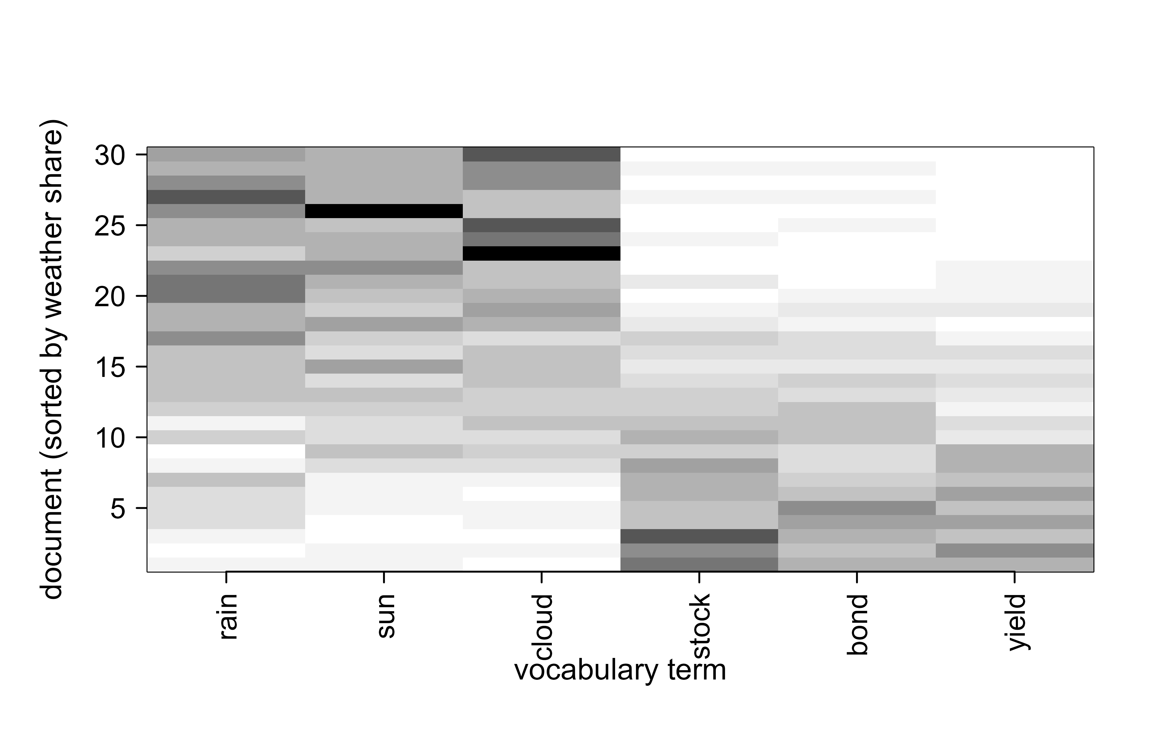
The block structure in Figure 34.2 is exactly what a topic model should recover: the upper documents (high weather share) load on the first three words, the lower documents on the last three.
34.8.2 A from-scratch collapsed Gibbs sampler
We now implement Equation 34.6 directly. The state is the topic assignment of every token; we maintain the count matrices \(n_{dk}\) (document-topic) and \(m_{kv}\) (topic-word) incrementally.
Show code
# Expand counts into a flat token list: (doc, word) pairs
tokens <- do.call(rbind, lapply(1:D, function(d)
  cbind(d, rep(1:V, times = C[d, ]))))
colnames(tokens) <- c("doc", "word")
Ntok <- nrow(tokens)

alpha <- 0.1; eta <- 0.01
z <- sample(1:K, Ntok, replace = TRUE)          # initial random assignments

# Count tables
n_dk <- matrix(0, D, K); m_kv <- matrix(0, K, V); n_k <- integer(K)
for (i in 1:Ntok) {
  d <- tokens[i, "doc"]; v <- tokens[i, "word"]; k <- z[i]
  n_dk[d, k] <- n_dk[d, k] + 1
  m_kv[k, v] <- m_kv[k, v] + 1
  n_k[k]     <- n_k[k] + 1
}

set.seed(7)
for (sweep in 1:400) {
  for (i in 1:Ntok) {
    d <- tokens[i, "doc"]; v <- tokens[i, "word"]; k <- z[i]
    # remove current token from counts
    n_dk[d, k] <- n_dk[d, k] - 1; m_kv[k, v] <- m_kv[k, v] - 1; n_k[k] <- n_k[k] - 1
    # collapsed Gibbs conditional, Eq. (topic-models-gibbs)
    prob <- (n_dk[d, ] + alpha) * (m_kv[, v] + eta) / (n_k + V * eta)
    k_new <- sample.int(K, 1, prob = prob)
    # re-add with the new assignment
    z[i] <- k_new
    n_dk[d, k_new] <- n_dk[d, k_new] + 1
    m_kv[k_new, v] <- m_kv[k_new, v] + 1
    n_k[k_new]     <- n_k[k_new] + 1
  }
}
34.8.3 Recovering and checking the topics
Plugging the final counts into the posterior means Equation 34.7 gives the estimated topic-word matrix \(\hat\beta\) and document-topic matrix \(\hat\theta\). Because topic labels are arbitrary, we align the recovered topics to the truth by matching whichever estimated topic best correlates with the weather topic.
Show code
beta_hat <- (m_kv + eta) / rowSums(m_kv + eta)
theta_hat <- (n_dk + alpha) / rowSums(n_dk + alpha)

# Align recovered topics to truth (labels are exchangeable)
if (cor(beta_hat[1, ], beta_true[1, ]) < cor(beta_hat[2, ], beta_true[1, ])) {
  beta_hat <- beta_hat[2:1, ]; theta_hat <- theta_hat[, 2:1]
}
rownames(beta_hat) <- c("weather (est.)", "finance (est.)")
knitr::kable(round(beta_hat, 3))| weather (est.) | 0.319 | 0.283 | 0.333 | 0.015 | 0.027 | 0.024 |
| finance (est.) | 0.076 | 0.061 | 0.036 | 0.326 | 0.257 | 0.244 |
Table 34.1 shows that the sampler recovers the two vocabularies cleanly, with each estimated topic placing nearly all its mass on the correct three words. The recovered document mixtures should likewise track the true weather shares used to generate each document.
Show code
plot(w_share, theta_hat[, 1], pch = 19, col = "steelblue",
     xlab = "true weather share", ylab = "estimated weather share (theta-hat)",
     xlim = c(0, 1), ylim = c(0, 1))
abline(0, 1, col = "grey50", lty = 2)
legend("topleft", bty = "n",
       legend = sprintf("correlation = %.2f", cor(w_share, theta_hat[, 1])))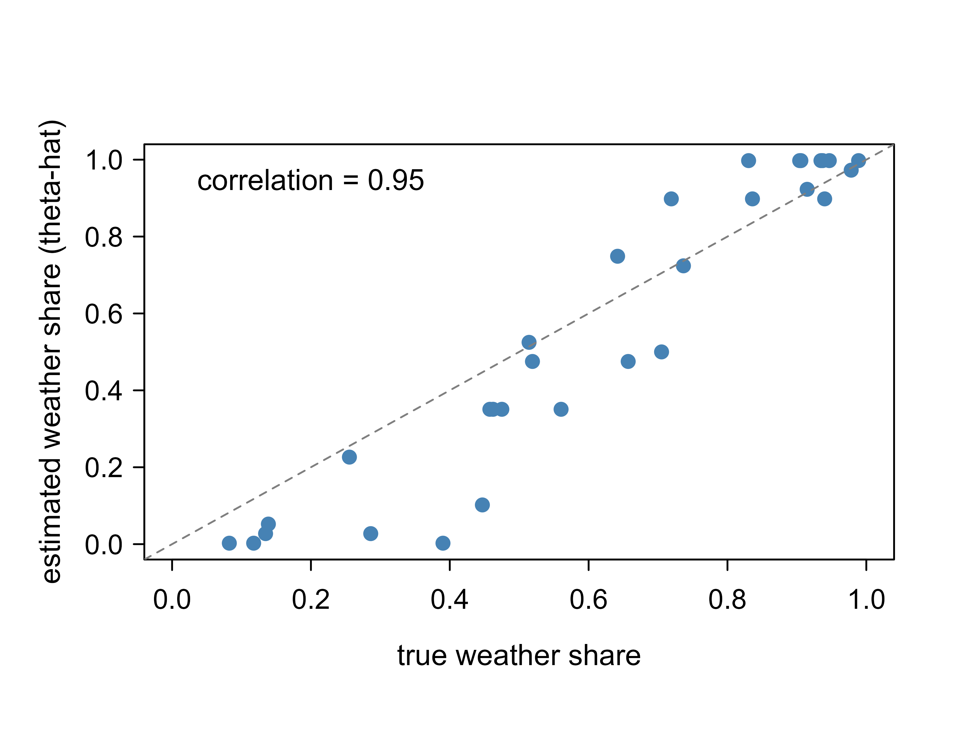
The tight scatter around the diagonal in Figure 34.3 is the headline result: from word counts alone, with no labels and a few hundred sampler sweeps, LDA reconstructs both the shared topic vocabularies and the per-document blends that produced the corpus.
34.8.4 A fixed reconstruction check
Finally, to make the factorization view of Equation 34.13 concrete, we reconstruct the expected word distribution per document, \(\hat\theta \hat\beta\), and compare it to the empirical word frequencies. A good fit means the rank-\(K\) product reproduces the observed counts.
Show code
| term | MAE |
|---|---|
| rain | 0.052 |
| sun | 0.034 |
| cloud | 0.051 |
| stock | 0.028 |
| bond | 0.033 |
| yield | 0.031 |
The small per-term errors in Table 34.2 confirm that the documents-by-topics times topics-by-words product reproduces the observed frequencies, which is precisely the low-rank factorization that LDA, pLSA, and NMF all share.
34.9 Further reading
Blei, Ng, and Jordan (2003) is the original LDA paper and remains the clearest derivation of the variational bound. Griffiths and Steyvers (2004) introduced the collapsed Gibbs sampler implemented above and is the most readable account of the count-based updates. Hoffman, Blei, and Bach (2010) developed online (stochastic) variational inference, the algorithm behind large-scale LDA. For the evaluation side, Chang et al. (2009) is the influential study showing perplexity and human interpretability can diverge, motivating coherence measures. On the lineage, Hofmann (1999) introduced pLSA, and the equivalence between KL-NMF and pLSA is treated by Gaussier and Goutte (2005). The review by Blei (2012) surveys topic models broadly, including the correlated, dynamic, and supervised variants that extend the basic model in this chapter.