51  Weakly-Supervised and Positive-Unlabeled Learning

51.1 Intuition

Standard supervised learning assumes a clean training table: every row carries an input \(x\) and a correct label \(y\). Reality is messier. A fraud team has a handful of confirmed frauds and a vast pile of transactions nobody ever investigated. A medical record system flags the patients who were diagnosed with a disease, but silence in the record does not mean a patient is healthy, it may just mean nobody checked. A content moderation pipeline relies on a few keyword rules and a noisy crowd-sourced vote rather than gold-standard adjudication. In each case we want a classifier, but the supervision we actually have is incomplete, inexact, or noisy.

Weak supervision is the umbrella term for learning under that kind of imperfect signal. Zhou (2018) organizes it into three flavors that we will keep returning to:

• Incomplete supervision: only a subset of the training data is labeled. Semi-supervised learning (Chapter 48) and positive-unlabeled (PU) learning live here.
• Inexact supervision: labels exist but at the wrong granularity, for example a label on a bag of instances rather than on each instance (multiple-instance learning).
• Inaccurate supervision: labels exist for everything but some are wrong (learning with label noise).

Intuition

Think of the label as a measurement of the truth taken through a dirty lens. Sometimes the lens only shows part of the picture (incomplete), sometimes it blurs fine detail into a coarse summary (inexact), and sometimes it reports the wrong reading entirely (inaccurate). Weakly-supervised learning is the discipline of recovering a sharp model from blurry measurements, by writing down how the lens distorts and then inverting it.

This chapter concentrates on two threads that a working data scientist meets often. The first is positive-unlabeled learning, the incomplete-label case where you observe some positives and a mass of unlabeled examples but never a single confirmed negative. The second is programmatic (weak) supervision, where instead of hand labels you write many noisy labeling rules and let a label model reconcile them. Along the way we treat label noise directly, since it is the mechanism underneath both. By the end you will be able to derive why a naive classifier trained on “positive versus unlabeled” is biased, correct that bias two different ways, and run a simulation that recovers a fully-supervised baseline from positives and unlabeled data alone.

51.2 Notation and the Selected-Completely-at-Random Model

We want a binary classifier. Let \(x \in \mathbb{R}^p\) be the input and \(y \in \{0, 1\}\) the true class, with \(y = 1\) the positive class. The clean joint distribution is \(p(x, y)\), and the quantity we ultimately care about is the posterior \(f(x) = p(y = 1 \mid x)\) or, equivalently, a decision rule derived from it.

In PU learning we never observe \(y\) directly. Instead we observe a labeling indicator \(s \in \{0, 1\}\): \(s = 1\) means “this example was selected and revealed to be positive,” and \(s = 0\) means “unlabeled.” The defining structural fact of the PU setting is

\[ s = 1 \;\Longrightarrow\; y = 1 , \]

that is, anything labeled is genuinely positive, but \(s = 0\) tells us nothing, the example could be a hidden positive or a true negative.

To make progress we need an assumption about which positives get labeled. The standard one is Selected Completely At Random (SCAR), due to Elkan and Noto (2008): a positive example is labeled with a constant probability that does not depend on its features,

\[ c \;=\; p(s = 1 \mid y = 1, x) \;=\; p(s = 1 \mid y = 1) . \]

The constant \(c\) is called the label frequency or propensity. SCAR says the lens that hides labels is uniform: it does not preferentially reveal easy positives or hard ones.

Key idea

SCAR turns an apparently hopeless problem (no negatives anywhere) into a solvable one. If labeled positives are a representative random sample of all positives, then the unlabeled pool is a known mixture of the same positives (the unlabeled fraction of them) and the negatives, and that mixture structure is enough to back out the clean classifier.

Warning

SCAR is an assumption, not a fact. If positives are labeled in a feature-dependent way (say, sicker patients are more likely to get diagnosed), the propensity becomes \(c(x)\) and plain SCAR estimators are biased. The weaker SAR (selected at random given features) model of Bekker and Davis (2020) handles that case but needs a propensity model, much like inverse-propensity weighting in causal machine learning (Chapter 76).

51.3 Why the Naive Classifier Is Biased, and How to Fix It

The tempting shortcut is to treat \(s\) as if it were \(y\): call labeled points positive, call everything unlabeled negative, and train an ordinary classifier. This is the nontraditional or naive PU classifier. It learns \(g(x) = p(s = 1 \mid x)\) rather than the target \(f(x) = p(y = 1 \mid x)\). The two are not equal, but under SCAR they are tied by a clean constant.

51.3.1 Elkan-Noto: the posterior is off by a constant factor

Start from the definition of the propensity and expand \(p(s = 1 \mid x)\) using \(s = 1 \Rightarrow y = 1\):

\[ g(x) = p(s = 1 \mid x) = p(y = 1, s = 1 \mid x) = p(y = 1 \mid x)\, p(s = 1 \mid y = 1, x) . \]

Under SCAR the last factor is the constant \(c\), so

\[ g(x) = c \cdot f(x) \qquad\Longleftrightarrow\qquad f(x) = \frac{g(x)}{c} . \]

This is the central result of Elkan and Noto (2008): the classifier you can actually fit, \(g\), is a scaled-down version of the one you want, \(f\). The labeled-versus-unlabeled probabilities are uniformly shrunk by the propensity \(c\). Two practical consequences follow.

First, if you only need a ranking or a thresholded decision, you do not even need \(c\), since dividing by a positive constant preserves the order of scores. The naive classifier already ranks correctly under SCAR. You only need \(c\) when you want calibrated probabilities or a threshold tied to a true positive rate.

Second, you can estimate \(c\) from a validation set. Take a held-out set of labeled positives \(P_{\text{val}}\). On such a point \(g(x) = c \cdot f(x)\), but note that \(f(x) = p(y=1\mid x)\) need not equal \(1\) even at a point known to be positive, because the classes overlap in feature space. Averaging the naive model’s score over known positives,

\[ \hat c \;=\; \frac{1}{|P_{\text{val}}|} \sum_{x \in P_{\text{val}}} \hat g(x) , \]

therefore estimates \(c\,\mathbb{E}[f(x)\mid y=1]\) (Elkan-Noto’s “e1” estimator), not \(c\) itself. It is exact only when the classes are (near-)separable, so that \(f(x)\approx 1\) on labeled positives, and it underestimates \(c\) whenever the classes overlap. When that bias matters, use a separability-robust estimator (Elkan-Noto’s “e3”) or recover \(c\) from \(\hat c = \hat p(s{=}1)/\hat\pi\) when the prior \(\pi\) is available.

Intuition

A known positive should score \(1\) under the true model \(f\). If the naive model \(g\) scores it only \(0.3\) on average, the lens is letting through about \(30\%\) of positives, so \(\hat c \approx 0.3\) and you divide every naive score by \(0.3\) to undo the shrinkage.

51.3.2 How the propensity and the prior are linked

The two nuisance constants of PU learning, the propensity \(c = p(s=1 \mid y=1)\) and the class prior \(\pi = p(y=1)\), are not independent. They are tied through the one quantity you can always observe directly: the labeled fraction \(p(s=1)\). Marginalizing over \(y\) and using \(s=1 \Rightarrow y=1\),

\[ p(s=1) = p(s=1, y=1) = p(s=1 \mid y=1)\,p(y=1) = c\,\pi . \tag{51.1}\]

The left side is estimated with no assumptions by the empirical labeled rate \(\hat p(s=1) = |P| / (|P| + |U|)\), where \(|P|\) counts labeled positives and \(|U|\) the unlabeled pool. Equation Equation 51.1 therefore says that knowing either constant pins down the other: \(\pi = p(s=1)/c\) and \(c = p(s=1)/\pi\). Estimating \(c\) on held-out positives (the Elkan-Noto recipe) implicitly fixes the prior at \(\hat\pi = \hat p(s=1)/\hat c\), and conversely a risk-based estimator that takes \(\pi\) as input implies a propensity \(\hat c = \hat p(s=1)/\hat\pi\). This is the precise sense in which the callout below means “estimating one constrains the other.”

There is a second Elkan-Noto estimator that exposes its variance properties. Because \(g(x)=c\,f(x)\), the held-out average computes \(\mathbb{E}_{x\sim p(\cdot\mid y=1)}[g(x)] = c\,\mathbb{E}[f(x)\mid y=1] \le c\), with equality iff \(f(x)=1\) almost surely on positives. So the held-out average \(\hat c = |P_{\text{val}}|^{-1}\sum_{x\in P_{\text{val}}} \hat g(x)\) targets \(c\,\mathbb{E}[f(x)\mid y=1]\), not \(c\) itself. Since each \(\hat g(x)\in[0,1]\), the estimator has variance \(\mathrm{Var}(\hat c) = \mathrm{Var}(g(x)\mid y=1)/|P_{\text{val}}| \le c(1-c)/|P_{\text{val}}|\), so it is \(\sqrt{|P_{\text{val}}|}\)-consistent for its target. The class overlap that spreads \(g\) over \([0,1]\) on positives is precisely what pulls \(\mathbb{E}[f(x)\mid y=1]\) below \(1\), so it both biases \(\hat c\) downward (the mean falls below \(c\)) and loosens this variance bound; when positives are cleanly separable, \(g\approx c\) on every positive and \(\hat c\) is both nearly unbiased and tight. A small validation set of positives is the usual bottleneck, because dividing every score by a noisy \(\hat c\) injects a multiplicative error \(c/\hat c\) into the entire calibration.

51.3.3 The class-prior view and the nnPU risk

A second route reframes PU learning as learning from class priors. Let \(\pi = p(y = 1)\) be the true positive prior. The unlabeled distribution is a mixture,

\[ p_{\text{u}}(x) = \pi\, p(x \mid y = 1) + (1 - \pi)\, p(x \mid y = 0) , \]

so the negative density we can never sample directly is implicitly \((1 - \pi)\, p(x \mid y = 0) = p_{\text{u}}(x) - \pi\, p(x \mid y = 1)\). Du Plessis, Niu, and Sugiyama (2014, 2015) used this to rewrite the supervised classification risk using only positive and unlabeled data. For a loss \(\ell\) and score function \(h\), the risk decomposes as

\[ R(h) = \pi\, \mathbb{E}_{p}\big[\ell(h(x), +1)\big] \;+\; \underbrace{\Big( \mathbb{E}_{\text{u}}\big[\ell(h(x), -1)\big] - \pi\, \mathbb{E}_{p}\big[\ell(h(x), -1)\big] \Big)}_{\text{estimated negative risk}} , \]

where \(\mathbb{E}_p\) averages over labeled positives and \(\mathbb{E}_{\text{u}}\) over the unlabeled pool. The bracketed term estimates the negative-class risk by subtracting the positive contribution out of the unlabeled mixture. This is the unbiased PU (uPU) risk. Its flaw: with a flexible model the bracketed estimate can go negative, which is impossible for a real risk and signals overfitting. Kiryo, Niu, du Plessis, and Sugiyama (2017) fixed this by clamping the negative-risk term at zero, giving the non-negative PU (nnPU) risk that is the default for deep PU models built on neural networks (Chapter 15) today.

51.3.3.1 Deriving the unbiased risk

Write the clean risk of a score \(h\) under loss \(\ell\), with the convention that \(\ell(h(x),+1)\) penalizes calling \(x\) positive-class and \(\ell(h(x),-1)\) penalizes calling it negative-class. Splitting by the true label and using \(\pi = p(y=1)\),

\[ R(h) = \pi\,\mathbb{E}_{p}[\ell(h(x),+1)] + (1-\pi)\,\mathbb{E}_{n}[\ell(h(x),-1)] , \tag{51.2}\]

where \(\mathbb{E}_p\) and \(\mathbb{E}_n\) are expectations under the class-conditional densities \(p(x\mid y{=}1)\) and \(p(x\mid y{=}0)\). The first term is estimable: we have labeled positives. The obstacle is \((1-\pi)\,\mathbb{E}_n[\cdot]\), since we never sample the negative density. The PU trick rewrites it using only the marginal mixture. From

\[ p_{\text{u}}(x) = \pi\,p(x\mid y{=}1) + (1-\pi)\,p(x\mid y{=}0) \]

we get, for any integrable test function \(\phi\),

\[ (1-\pi)\,\mathbb{E}_n[\phi] = \mathbb{E}_{\text{u}}[\phi] - \pi\,\mathbb{E}_p[\phi] , \tag{51.3}\]

simply by integrating \(\phi\) against both sides of the mixture and rearranging. Setting \(\phi(x)=\ell(h(x),-1)\) and substituting into Equation 51.2 gives the uPU risk

\[ \widehat{R}_{\text{uPU}}(h) = \pi\,\mathbb{E}_{p}[\ell(h(x),+1)] + \Big(\mathbb{E}_{\text{u}}[\ell(h(x),-1)] - \pi\,\mathbb{E}_{p}[\ell(h(x),-1)]\Big) , \]

which is exactly the displayed estimator above. The construction is unbiased by Equation 51.3: \(\mathbb{E}[\widehat{R}_{\text{uPU}}(h)] = R(h)\) for every fixed \(h\), with no SCAR-specific step beyond knowing \(\pi\).

51.3.3.2 Why the bracket goes negative, and the nnPU fix

The bracketed estimator of the negative risk, \(\widehat{R}_n^-(h) = \mathbb{E}_{\text{u}}[\ell(h(x),-1)] - \pi\,\mathbb{E}_{p}[\ell(h(x),-1)]\), estimates a true risk \((1-\pi)\,\mathbb{E}_n[\ell(h(x),-1)] \ge 0\). But it is a difference of two empirical averages, and with a high-capacity \(h\) that drives \(\ell(h(x),-1)\) near zero on the unlabeled sample while it stays positive on the positive sample, the empirical bracket can dip below zero. That is impossible for a real nonnegative risk; it is the signature of overfitting, and minimizing an unbounded-below objective lets training diverge. Kiryo et al. (2017) clamp it:

\[ \widehat{R}_{\text{nnPU}}(h) = \pi\,\mathbb{E}_{p}[\ell(h(x),+1)] + \max\!\Big\{0,\ \mathbb{E}_{\text{u}}[\ell(h(x),-1)] - \pi\,\mathbb{E}_{p}[\ell(h(x),-1)]\Big\} . \tag{51.4}\]

In practice the maximum is applied per minibatch; when a batch’s bracket is negative, the optimizer takes a gradient-ascent step on that term instead (deliberately worsening fit there) to climb back into the feasible region. The clamp introduces a small downward bias in the estimated risk (Jensen’s inequality applied to \(\max\{0,\cdot\}\), a convex function, gives \(\mathbb{E}[\max\{0,Z\}] \ge \max\{0,\mathbb{E}[Z]\}\), so the clamped risk overestimates the negative risk slightly), but it sharply reduces variance and, critically, restores a lower bound so the objective cannot diverge. Kiryo et al. prove the nnPU estimator is biased but its estimation error still shrinks at the parametric rate: with \(n_p\) positives and \(n_u\) unlabeled, the deviation of the empirical minimizer’s risk from the optimum is \(O_p(1/\sqrt{n_p} + 1/\sqrt{n_u})\) for a function class of bounded Rademacher complexity. The bias decays exponentially in those sample sizes, so for moderate data the nnPU minimizer is effectively as good as the (lower-variance) corrected estimator while never overfitting into negative-risk territory.

Warning

The uPU and nnPU risks need the prior \(\pi\) as a known input. A wrong \(\pi\) biases the correction: too large a \(\pi\) oversubtracts the positive contribution and pushes the negative-risk estimate down (more clamping, more bias); too small a \(\pi\) undercorrects and the model drifts back toward the naive classifier. Mixture-proportion estimation (for example the methods surveyed by Bekker and Davis, 2020) supplies \(\hat\pi\) from PU data alone, but it is the most fragile step in the pipeline and deserves a sensitivity check.

Note

The two corrections answer different questions. Elkan-Noto post-processes a single naive model’s scores by a constant and needs the propensity \(c\). The risk-based view rebuilds the loss from scratch and needs the prior \(\pi\). They are connected: under SCAR, \(c\) and \(\pi\) are related through the observed labeled fraction, so estimating one constrains the other.

51.4 A Runnable PU Demo Versus a Supervised Baseline

We now make the Elkan-Noto correction concrete. The plan: simulate a two-class problem where the truth is known, hide most positive labels and all negatives to create a PU dataset, train three classifiers (an oracle that cheats with the true labels, a naive PU classifier, and the corrected one), and compare them on a clean test set. Everything runs in base R plus glmnet-free logistic regression via glm.

set.seed(2026)

# Simulate two Gaussian classes in 2D with partial overlap.
simulate_data <- function(n, pi_pos = 0.4) {
  npos <- rbinom(1, n, pi_pos)
  nneg <- n - npos
  pos <- cbind(rnorm(npos, 2.0, 1.0), rnorm(npos, 2.0, 1.0))
  neg <- cbind(rnorm(nneg, 0.0, 1.0), rnorm(nneg, 0.0, 1.0))
  X <- rbind(pos, neg)
  y <- c(rep(1L, npos), rep(0L, nneg))
  idx <- sample(nrow(X))
  data.frame(x1 = X[idx, 1], x2 = X[idx, 2], y = y[idx])
}

train_full <- simulate_data(2000, pi_pos = 0.4)
test_set   <- simulate_data(4000, pi_pos = 0.4)

# Build the PU labeling under SCAR: label each positive with prob c.
c_true <- 0.30
train_pu <- train_full
reveal <- with(train_pu, y == 1 & runif(nrow(train_pu)) < c_true)
train_pu$s <- as.integer(reveal)   # s = 1 labeled positive, else unlabeled

cat(sprintf("True positives: %d | Revealed (s=1): %d | Unlabeled: %d\n",
            sum(train_full$y), sum(train_pu$s), sum(train_pu$s == 0)))
#> True positives: 819 | Revealed (s=1): 232 | Unlabeled: 1768

The oracle uses the hidden truth y. The naive and corrected models see only s.

# 1. Oracle: logistic regression on the TRUE labels (upper bound).
fit_oracle <- glm(y ~ x1 + x2, family = binomial, data = train_full)

# 2. Naive PU: treat s as the label (labeled = 1, unlabeled = 0).
fit_naive <- glm(s ~ x1 + x2, family = binomial, data = train_pu)

# 3. Elkan-Noto correction. Estimate c on held-out known positives,
#    then divide naive scores by c_hat to recover f(x) = p(y=1|x).
known_pos <- train_pu[train_pu$s == 1, ]
g_on_pos  <- predict(fit_naive, newdata = known_pos, type = "response")
c_hat     <- mean(g_on_pos)

predict_corrected <- function(model, newdata, c_hat) {
  g <- predict(model, newdata = newdata, type = "response")
  pmin(g / c_hat, 1)          # f(x) = g(x)/c, clipped into [0,1]
}

cat(sprintf("True c = %.3f | Estimated c_hat = %.3f\n", c_true, c_hat))
#> True c = 0.300 | Estimated c_hat = 0.232

Now score all three on the clean test set and report accuracy and AUC. We use a small self-contained AUC function so no extra package is required.

auc <- function(scores, labels) {
  pos <- scores[labels == 1]
  neg <- scores[labels == 0]
  # Probability a random positive outranks a random negative (Mann-Whitney).
  r <- rank(c(pos, neg))
  (sum(r[seq_along(pos)]) - length(pos) * (length(pos) + 1) / 2) /
    (length(pos) * length(neg))
}

p_oracle    <- predict(fit_oracle, test_set, type = "response")
p_naive     <- predict(fit_naive,  test_set, type = "response")
p_corrected <- predict_corrected(fit_naive, test_set, c_hat)

acc <- function(p, y, thr = 0.5) mean((p >= thr) == (y == 1))

results <- data.frame(
  Model    = c("Oracle (true labels)", "Naive PU (s as label)",
               "Corrected PU (Elkan-Noto)"),
  AUC      = c(auc(p_oracle, test_set$y),
               auc(p_naive, test_set$y),
               auc(p_corrected, test_set$y)),
  Accuracy = c(acc(p_oracle, test_set$y),
               acc(p_naive, test_set$y),
               acc(p_corrected, test_set$y))
)
results$AUC      <- round(results$AUC, 3)
results$Accuracy <- round(results$Accuracy, 3)
print(results)
#>                       Model   AUC Accuracy
#> 1      Oracle (true labels) 0.973    0.917
#> 2     Naive PU (s as label) 0.973    0.612
#> 3 Corrected PU (Elkan-Noto) 0.973    0.902

Table 51.1 reports the numbers in a formatted comparison.

knitr::kable(
  results,
  caption = "Test-set performance of an oracle classifier (trained on true labels), a naive PU classifier that treats the labeling indicator as the label, and the Elkan-Noto corrected classifier. AUC is rank-based and so is nearly identical across naive and corrected models, as the theory predicts; the threshold-based accuracy is where the constant correction matters."
)

Table 51.1: Test-set performance of an oracle classifier (trained on true labels), a naive PU classifier that treats the labeling indicator as the label, and the Elkan-Noto corrected classifier. AUC is rank-based and so is nearly identical across naive and corrected models, as the theory predicts; the threshold-based accuracy is where the constant correction matters.

Model	AUC	Accuracy
Oracle (true labels)	0.973	0.917
Naive PU (s as label)	0.973	0.612
Corrected PU (Elkan-Noto)	0.973	0.902

Two things should stand out in Table 51.1. The AUC of the naive and corrected models is essentially identical, because dividing every score by the same constant \(\hat c\) cannot change the ranking, exactly as the derivation \(f = g / c\) implies. The accuracy at the default \(0.5\) threshold is where they diverge: the naive model’s scores are squashed toward zero (almost nothing crosses \(0.5\), so it under-predicts the positive class), while the corrected model rescales them back into a usable range close to the oracle.

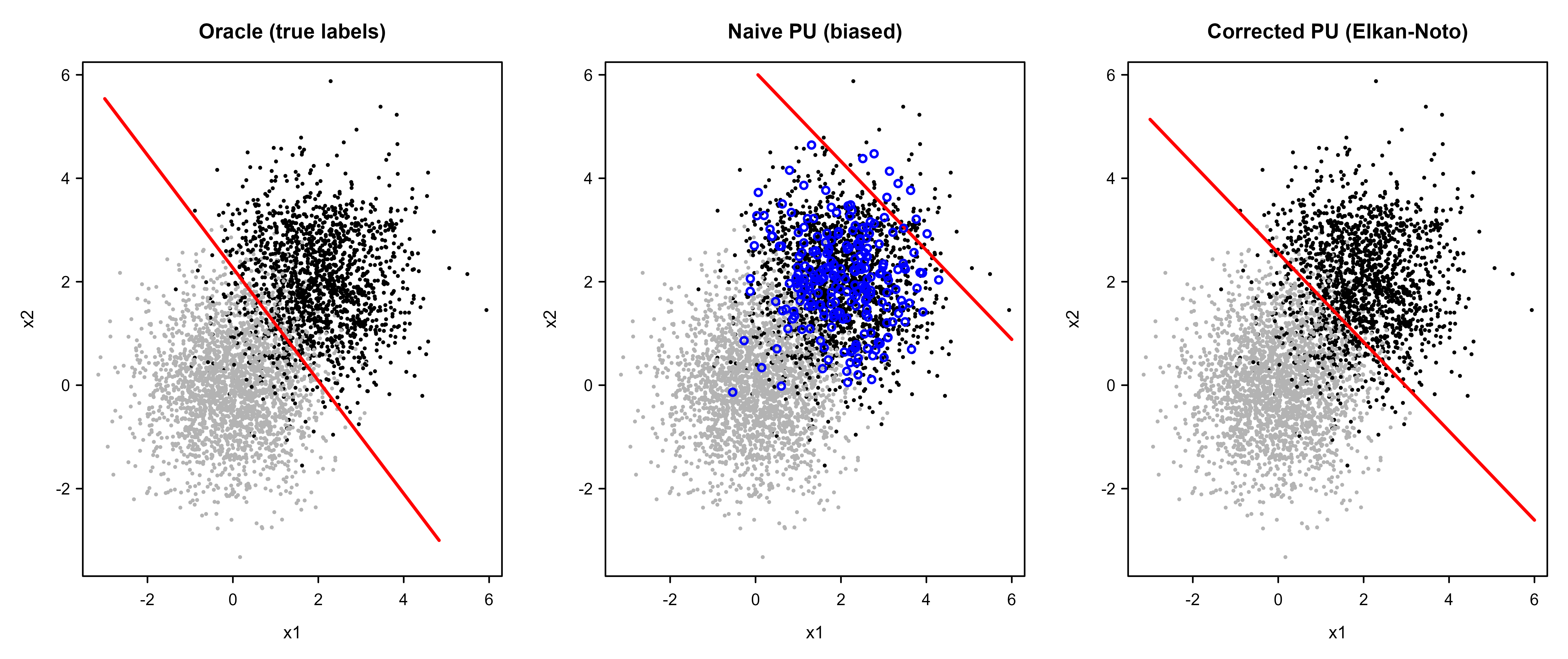
The figure makes the rescaling visible by comparing the three decision boundaries in feature space.

grid <- expand.grid(
  x1 = seq(-3, 6, length.out = 200),
  x2 = seq(-3, 6, length.out = 200)
)
z_oracle    <- matrix(predict(fit_oracle, grid, type = "response"), 200, 200)
z_naive     <- matrix(predict(fit_naive,  grid, type = "response"), 200, 200)
z_corrected <- matrix(predict_corrected(fit_naive, grid, c_hat),    200, 200)
gx <- sort(unique(grid$x1)); gy <- sort(unique(grid$x2))

old_par <- par(mfrow = c(1, 3), mar = c(4, 4, 3, 1))
plot_panel <- function(z, title, show_revealed = FALSE) {
  plot(test_set$x1, test_set$x2,
       col = ifelse(test_set$y == 1, "black", "grey70"),
       pch = 19, cex = 0.3, xlab = "x1", ylab = "x2", main = title)
  contour(gx, gy, z, levels = 0.5, add = TRUE, lwd = 2, col = "red",
          drawlabels = FALSE)
  if (show_revealed) {
    rp <- train_pu[train_pu$s == 1, ]
    points(rp$x1, rp$x2, pch = 1, cex = 0.9, col = "blue", lwd = 1.5)
  }
}
plot_panel(z_oracle,    "Oracle (true labels)")
plot_panel(z_naive,     "Naive PU (biased)", show_revealed = TRUE)
plot_panel(z_corrected, "Corrected PU (Elkan-Noto)")
par(old_par)

Figure 51.1: Decision boundaries on the simulated two-class problem. Grey points are true negatives, black points are true positives; the few revealed PU positives are circled in the right panel. The naive PU boundary sits far inside the positive cloud because its scores are shrunk by the propensity, so it labels almost everything negative. The Elkan-Noto correction moves the boundary back to nearly coincide with the oracle’s.

Figure 51.1 shows the geometric effect of the bias: the naive red curve is pushed deep into the positive cluster (it has learned \(g = c \cdot f\), a model that is “sure” only about the densest positive core), while the corrected curve snaps back almost on top of the oracle boundary. The blue circles in the middle panel are the handful of revealed positives the PU models were allowed to see.

Note

This demo uses logistic regression, but nothing about Elkan-Noto is tied to it. Any probabilistic classifier (random forest with type = "prob", gradient boosting, a neural net) can be wrapped the same way: fit on \(s\), estimate \(\hat c\) on held-out known positives, divide. The risk-based nnPU estimator is the alternative when you would rather change the loss than post-process the scores, and it is what you reach for with deep models.

51.5 Programmatic Weak Supervision and Label Models

PU learning assumes one weak signal (a partial positive label). Programmatic weak supervision, popularized by the Snorkel system (Ratner, Bach, Ehrenberg, Fries, Wu, and Ré, 2017), assumes the opposite: you have many weak signals and want to combine them. Instead of hand-labeling examples you write labeling functions (LFs), small heuristics that each vote a label or abstain. A spam LF might fire “spam” on any message containing a payment link, abstain otherwise. The LFs are noisy, they overlap, and they conflict. The job of a label model is to estimate each LF’s reliability and fuse their votes into a single probabilistic label per example, without ever seeing ground truth.

Formally, for example \(i\) each of \(m\) labeling functions emits a vote \(\lambda_{ij} \in \{-1, 0, +1\}\), where \(0\) means abstain. The data-programming model of Ratner, De Sa, Wu, Selsam, and Ré (2016) treats the unknown true label \(y_i\) as latent and posits that each LF is right with some accuracy and abstains with some rate. The simplest version assumes conditional independence of LFs given \(y\) (a Naive-Bayes-style assumption; see Chapter 18), giving

\[ p(\lambda_{i \cdot}, y_i) \;\propto\; p(y_i) \prod_{j=1}^{m} p(\lambda_{ij} \mid y_i) , \]

with the per-LF accuracies \(p(\lambda_{ij} \mid y_i)\) as parameters fit by maximizing the marginal likelihood of the observed votes (the \(y_i\) are integrated out, an EM-style estimation). The output is a soft label \(p(y_i = 1 \mid \lambda_{i\cdot})\) per example, which then trains a downstream “end model” exactly as if it were a noisy ground-truth label.

51.5.0.1 The EM updates, derived

Parameterize each LF \(j\) by an abstain rate \(\beta_j = p(\lambda_{ij}=0)\) and a conditional accuracy \(\alpha_j = p(\lambda_{ij}=y_i \mid \lambda_{ij}\neq 0)\), with class prior \(\pi=p(y_i=1)\). The observed-data log-likelihood marginalizes the latent label,

\[ \ell(\theta) = \sum_{i=1}^{n} \log \sum_{y\in\{0,1\}} p(y)\prod_{j=1}^{m} p(\lambda_{ij}\mid y) , \]

which is not concave in \(\theta=(\pi,\alpha,\beta)\) because of the sum inside the log. EM optimizes it by alternating a tractable lower bound. Introduce the responsibility \(r_i = p(y_i=1\mid \lambda_{i\cdot};\theta)\).

E-step. By Bayes’ rule under conditional independence,

\[ r_i = \frac{\pi\prod_j p(\lambda_{ij}\mid y{=}1)}{\pi\prod_j p(\lambda_{ij}\mid y{=}1) + (1-\pi)\prod_j p(\lambda_{ij}\mid y{=}0)} . \tag{51.5}\]

Abstentions (\(\lambda_{ij}=0\)) contribute the same factor \(\beta_j\) to numerator and denominator and so cancel, which is why the code adds \(0\) to the log-likelihood on abstain and only non-abstaining votes move the posterior. This is the source of the logistic-style update in the demo: working in log space, \(\log r_i - \log(1-r_i) = \mathrm{logit}(\pi) + \sum_{j:\lambda_{ij}\neq 0} \big(\mathbf{1}[\lambda_{ij}=1]-\mathbf{1}[\lambda_{ij}=-1]\big)\,\log\frac{\alpha_j}{1-\alpha_j}\), so each firing LF casts a vote weighted by its log-accuracy-odds, and the demo recovers \(r_i\) via the sigmoid of this log-odds.

M-step. Maximize the expected complete-data log-likelihood \(Q(\theta) = \sum_i \mathbb{E}_{y_i\sim r_i}[\log p(y_i) + \sum_j \log p(\lambda_{ij}\mid y_i)]\). The terms separate, so each parameter has a closed form. Setting \(\partial Q/\partial\pi = 0\) gives \(\hat\pi = \frac1n\sum_i r_i\). For \(\alpha_j\), a firing vote is “correct” with responsibility-weighted indicator \(w_{ij} = r_i\mathbf{1}[\lambda_{ij}=1] + (1-r_i)\mathbf{1}[\lambda_{ij}=-1]\), and maximizing the Bernoulli log-likelihood over fired examples yields

\[ \hat\alpha_j = \frac{\sum_{i:\lambda_{ij}\neq 0} w_{ij}}{\sum_{i:\lambda_{ij}\neq 0} 1} , \qquad \hat\beta_j = \frac1n\sum_{i} \mathbf{1}[\lambda_{ij}=0] . \tag{51.6}\]

The accuracy update Equation 51.6 is exactly the M-step the demo computes (“expected fraction of correct non-abstains”), and the abstain rate is just the empirical firing complement, which is why the demo never updates it. EM monotonically increases \(\ell(\theta)\) and converges to a stationary point; like all EM it is sensitive to initialization (the demo seeds every accuracy at \(0.7\)).

51.5.0.2 Identifiability and its failure mode

The likelihood has an exact symmetry: relabeling \(y\mapsto 1-y\) and \(\alpha_j\mapsto 1-\alpha_j\) for all \(j\) leaves every observed vote distribution unchanged. The model can only learn accuracies up to this global flip, so it cannot tell “all LFs are good” from “all LFs are systematically wrong.” Two conventions break it: assume each \(\alpha_j>1/2\) (LFs are better than chance), or pin orientation with a single labeled example. The deeper failure is the conditional-independence assumption: if a subset of LFs share an upstream resource (the same dictionary or parser), their errors correlate, the product in Equation 51.5 double-counts agreeing votes, and the label model becomes overconfident, assigning \(r_i\) near \(0\) or \(1\) on examples where the correlated cluster merely agrees with itself. Snorkel’s later “MeTaL” formulation models such dependencies as edges in a graphical model and estimates accuracies from the observed agreement covariance rather than full EM, which scales better and tolerates known correlations.

Key idea

Majority vote treats every labeling function as equally trustworthy. A label model learns from the agreement and disagreement structure of the votes which LFs to trust, even with no labeled data, because a consistently-outvoted LF reveals itself as unreliable. This is the same latent-variable trick as crowd-sourcing aggregation (Dawid and Skene, 1979).

Here is a compact base-R label model: estimate per-LF accuracies by EM and compare its fused label against plain majority vote.

set.seed(7)
n <- 3000; m <- 5
y_true <- rbinom(n, 1, 0.5)                       # latent truth (for eval only)
acc  <- c(0.90, 0.80, 0.70, 0.60, 0.55)           # true LF accuracies
abst <- c(0.10, 0.20, 0.30, 0.50, 0.40)           # true LF abstain rates

# Generate votes in {-1 (neg), 0 (abstain), 1 (pos)}.
lambda <- matrix(0L, n, m)
for (j in seq_len(m)) {
  fire <- runif(n) > abst[j]
  correct <- runif(n) < acc[j]
  vote_pos <- ifelse(correct, y_true == 1, y_true == 0)
  lambda[, j] <- ifelse(!fire, 0L, ifelse(vote_pos, 1L, -1L))
}

# Majority vote baseline (ties -> positive).
mv_score <- rowSums(lambda)
mv_pred  <- as.integer(mv_score >= 0)

# EM label model assuming conditional independence given y.
prior <- 0.5
a <- rep(0.7, m)                                  # init per-LF accuracy
for (iter in 1:50) {
  # E-step: posterior over y for each row given current accuracies.
  log_p1 <- log(prior); log_p0 <- log(1 - prior)
  ll1 <- rep(log_p1, n); ll0 <- rep(log_p0, n)
  for (j in seq_len(m)) {
    v <- lambda[, j]
    ll1 <- ll1 + ifelse(v == 0, 0, ifelse(v == 1, log(a[j]), log(1 - a[j])))
    ll0 <- ll0 + ifelse(v == 0, 0, ifelse(v == -1, log(a[j]), log(1 - a[j])))
  }
  post1 <- 1 / (1 + exp(ll0 - ll1))               # p(y=1 | votes)
  # M-step: re-estimate accuracy = expected fraction of correct non-abstains.
  for (j in seq_len(m)) {
    v <- lambda[, j]; fired <- v != 0
    agree_pos <- (v == 1)
    correct_w <- ifelse(agree_pos, post1, 1 - post1)
    a[j] <- sum(correct_w[fired]) / sum(fired)
  }
  prior <- mean(post1)
}
lm_pred <- as.integer(post1 >= 0.5)

lf_table <- data.frame(
  LF             = paste0("LF", 1:m),
  True_accuracy  = acc,
  Estimated_acc  = round(a, 3)
)
print(lf_table)
#>    LF True_accuracy Estimated_acc
#> 1 LF1          0.90         0.901
#> 2 LF2          0.80         0.808
#> 3 LF3          0.70         0.699
#> 4 LF4          0.60         0.623
#> 5 LF5          0.55         0.558

The label model recovers each labeling function’s hidden accuracy from votes alone, ranking the reliable LFs above the noisy ones. Table 51.2 shows the recovered accuracies, and the accuracy comparison against majority vote.

compare <- data.frame(
  Method = c("Majority vote", "EM label model"),
  Label_accuracy = round(c(mean(mv_pred == y_true),
                           mean(lm_pred == y_true)), 3)
)
knitr::kable(
  list(lf_table, compare),
  caption = "Left: per-labeling-function accuracies recovered by the EM label model from votes alone, next to the true (hidden) accuracies used to generate the data. Right: accuracy of the fused label from majority vote versus the EM label model, against held-out ground truth. The label model down-weights the unreliable functions and so beats the equal-weight majority vote."
)

Table 51.2

Left: per-labeling-function accuracies recovered by the EM label model from votes alone, next to the true (hidden) accuracies used to generate the data. Right: accuracy of the fused label from majority vote versus the EM label model, against held-out ground truth. The label model down-weights the unreliable functions and so beats the equal-weight majority vote.

LF True_accuracy Estimated_acc LF1 0.90 0.901 LF2 0.80 0.808 LF3 0.70 0.699 LF4 0.60 0.623 LF5 0.55 0.558

Method Label_accuracy Majority vote 0.837 EM label model 0.891

Table 51.2 shows the payoff of modeling reliability: the EM label model’s estimated accuracies track the true ones, and because it discounts the weak functions (LF4 and LF5) instead of giving them an equal vote, its fused labels are more accurate than majority vote.

51.6 Learning with Label Noise

Both threads above are special cases of a more general problem: the labels you train on differ from the truth. It is worth stating the noise model directly, because the same correction logic recurs. In the class-conditional noise model the observed label \(\tilde y\) flips from the true \(y\) with class-dependent rates

\[ \rho_{+} = p(\tilde y = 0 \mid y = 1), \qquad \rho_{-} = p(\tilde y = 1 \mid y = 0) . \]

PU learning under SCAR is exactly this model with \(\rho_{-} = 0\) (no negative is ever mislabeled positive, since \(s = 1 \Rightarrow y = 1\)) and \(\rho_{+} = 1 - c\) (a fraction \(1 - c\) of positives are “flipped” into the unlabeled pool). Natarajan, Dhillon, Ravikumar, and Tewari (2013) showed that if the flip rates are known, you can build an unbiased loss: define a corrected loss \(\tilde\ell\) on noisy labels whose expectation equals the clean loss,

\[ \tilde\ell(h(x), \tilde y) = \frac{(1 - \rho_{-\tilde y})\,\ell(h(x), \tilde y) - \rho_{\tilde y}\,\ell(h(x), -\tilde y)}{1 - \rho_{+} - \rho_{-}} , \]

so that minimizing average \(\tilde\ell\) on noisy data is equivalent to minimizing \(\ell\) on clean data. This is the same “subtract out the contamination, then renormalize” move as the uPU risk, and it is why the three topics in this chapter are really one idea applied through different noise lenses.

51.6.0.1 Deriving the unbiased correction

We want a surrogate \(\tilde\ell\) whose expectation over the noisy label, conditional on the true label, equals the clean loss: \(\mathbb{E}_{\tilde y\mid y}[\tilde\ell(h(x),\tilde y)] = \ell(h(x),y)\). Fix \(x\) and abbreviate \(\ell_{+}=\ell(h(x),+1)\), \(\ell_{-}=\ell(h(x),-1)\), and likewise \(\tilde\ell_{\pm}\), writing labels as \(\pm 1\). Condition on the true class. If \(y=+1\) the noisy label is \(+1\) with probability \(1-\rho_{+}\) and flips to \(-1\) with probability \(\rho_{+}\); if \(y=-1\) it is \(-1\) with probability \(1-\rho_{-}\) and flips to \(+1\) with probability \(\rho_{-}\). The unbiasedness requirement is the linear system

\[ \begin{aligned} (1-\rho_{+})\,\tilde\ell_{+} + \rho_{+}\,\tilde\ell_{-} &= \ell_{+},\\ \rho_{-}\,\tilde\ell_{+} + (1-\rho_{-})\,\tilde\ell_{-} &= \ell_{-}. \end{aligned} \tag{51.7}\]

This is two equations in the two unknowns \(\tilde\ell_{+},\tilde\ell_{-}\). The coefficient matrix has determinant \((1-\rho_{+})(1-\rho_{-}) - \rho_{+}\rho_{-} = 1-\rho_{+}-\rho_{-}\), which is nonzero precisely when the noise is not so severe that the labels become uninformative (\(\rho_{+}+\rho_{-}\neq 1\)). Solving by Cramer’s rule,

\[ \tilde\ell_{+} = \frac{(1-\rho_{-})\,\ell_{+} - \rho_{+}\,\ell_{-}}{1-\rho_{+}-\rho_{-}}, \qquad \tilde\ell_{-} = \frac{(1-\rho_{+})\,\ell_{-} - \rho_{-}\,\ell_{+}}{1-\rho_{+}-\rho_{-}} . \tag{51.8}\]

The two cases of Equation 51.8 are summarized by the single expression stated above, with \(\rho_{\tilde y}\) the flip rate out of the observed class and \(\rho_{-\tilde y}\) the flip rate into it. Because the correction is taken inside the expectation, \(\mathbb{E}_{\tilde y\mid y}[\tilde\ell] = \ell\) holds for every \(x\), so the empirical noisy risk is an unbiased estimator of the clean risk and its minimizer is consistent (Natarajan et al. 2013 give the matching estimation-error bound). The price is variance: the \(1/(1-\rho_{+}-\rho_{-})\) factor inflates the loss as noise approaches the uninformative boundary, so the corrected estimator is high-variance exactly when the labels are nearly useless. Note that \(\tilde\ell\) can be negative even when \(\ell\) is not, which is the same non-convexity hazard the nnPU clamp addresses, and a reminder that loss correction trades unbiasedness for stability.

Specializing to PU under SCAR (\(\rho_{-}=0\), \(\rho_{+}=1-c\)) collapses Equation 51.8 to \(\tilde\ell_{+}=\ell_{+}/c - (1-c)\ell_{-}/c\) and \(\tilde\ell_{-}=\ell_{-}\), the loss-space twin of the Elkan-Noto and uPU corrections: a positive label is the clean positive loss net of a discounted negative loss, scaled by \(1/c\), while an unlabeled point contributes only the negative loss. The three results are one identity viewed in posterior space, risk space, and loss space.

The following short simulation verifies Equation 51.8 numerically: averaging the corrected loss over noisy labels reproduces the clean loss.

set.seed(11)
rho_p <- 0.30; rho_n <- 0.15            # flip rates p(yt=0|y=1), p(yt=1|y=0)
ell_p <- 0.8; ell_n <- 0.2              # arbitrary clean losses l(h,+1), l(h,-1)
den <- 1 - rho_p - rho_n
# Corrected losses from eq-natarajan.
tl_p <- ((1 - rho_n) * ell_p - rho_p * ell_n) / den   # corrected loss for yt=+1
tl_n <- ((1 - rho_p) * ell_n - rho_n * ell_p) / den   # corrected loss for yt=-1

# Monte Carlo: draw noisy labels for a true positive and a true negative,
# average the corrected loss, and compare to the clean loss.
N <- 2e6
yt_pos <- ifelse(runif(N) < rho_p, -1, 1)             # true y = +1
yt_neg <- ifelse(runif(N) < rho_n,  1, -1)            # true y = -1
mc_pos <- mean(ifelse(yt_pos == 1, tl_p, tl_n))       # should equal ell_p
mc_neg <- mean(ifelse(yt_neg == 1, tl_p, tl_n))       # should equal ell_n
cat(sprintf("E[corrected | y=+1] = %.4f  (clean l_+ = %.4f)\n", mc_pos, ell_p))
#> E[corrected | y=+1] = 0.8001  (clean l_+ = 0.8000)
cat(sprintf("E[corrected | y=-1] = %.4f  (clean l_- = %.4f)\n", mc_neg, ell_n))
#> E[corrected | y=-1] = 0.2003  (clean l_- = 0.2000)

The two Monte Carlo averages match the clean losses to sampling error, confirming the correction is unbiased term by term.

When to use this

If you can estimate flip rates (from a small clean validation set, from a confident-learning procedure like Northcutt, Jiang, and Chuang 2021, or from domain knowledge), loss correction is principled and cheap. If you cannot, robust losses (for example the generalized cross-entropy of Zhang and Sabuncu 2018) or sample-reweighting heuristics are the fallback, trading the unbiasedness guarantee for not needing to know the rates.

51.7 Practical Guidance and Pitfalls

A few lessons recur across PU, programmatic supervision, and noisy labels.

Estimate the nuisance constant on held-out positives, not training positives. The propensity \(\hat c\) and the prior \(\hat \pi\) are the parameters that make or break PU calibration, and estimating them on the same points used to fit the model leaks optimism. Hold out a clean fold of known positives for \(\hat c\).

Check the SCAR assumption before trusting a single constant. If you suspect labeling depends on features (sicker patients diagnosed more often, popular items reviewed more often), SCAR is violated and a constant correction is wrong. Move to the SAR model with an explicit propensity \(c(x)\), or at minimum stratify \(\hat c\) within feature groups.

Warning

A naive PU classifier reports terrible accuracy and calibration even when its ranking is fine. Do not conclude PU learning failed because precision at threshold \(0.5\) is low. Look at AUC or average precision first, and only then worry about the threshold, which the propensity correction sets.

For programmatic supervision, write labeling functions to be precise where they fire and free to abstain. A high-coverage but inaccurate LF poisons the label model less than you might fear (the model down-weights it), but a systematically correlated set of LFs breaks the conditional-independence assumption and inflates apparent confidence. Audit LF pairwise agreement, and model correlations when LFs share an upstream resource (the same dictionary, the same parser).

Match the prior to your deployment, not your sample. PU and noisy-label corrections both depend on the class prior \(\pi\). If your unlabeled pool was collected under a different positive rate than production, the correction will be miscalibrated in production. Re-estimate \(\pi\) on a target-domain sample when domains shift.

Finally, do not over-engineer. The Elkan-Noto correction is two lines on top of any classifier and is often enough. Reach for nnPU, confident learning, or a full label model when the simple constant correction is demonstrably insufficient, not by default.

51.8 Further Reading

• Elkan, C., and Noto, K. (2008). Learning classifiers from only positive and unlabeled data. The original SCAR analysis and the \(f = g/c\) correction used in this chapter.
• du Plessis, M. C., Niu, G., and Sugiyama, M. (2014, 2015). Analysis of learning from positive and unlabeled data and the unbiased PU risk estimator.
• Kiryo, R., Niu, G., du Plessis, M. C., and Sugiyama, M. (2017). Positive-unlabeled learning with non-negative risk estimator (nnPU).
• Bekker, J., and Davis, J. (2020). Learning from positive and unlabeled data: a survey. A thorough modern overview including the SAR model.
• Ratner, A., De Sa, C., Wu, S., Selsam, D., and Ré, C. (2016). Data programming: creating large training sets, quickly.
• Ratner, A., Bach, S. H., Ehrenberg, H., Fries, J., Wu, S., and Ré, C. (2017). Snorkel: rapid training data creation with weak supervision.
• Dawid, A. P., and Skene, A. M. (1979). Maximum likelihood estimation of observer error-rates using the EM algorithm. The latent-variable label-aggregation ancestor of label models.
• Natarajan, N., Dhillon, I. S., Ravikumar, P., and Tewari, A. (2013). Learning with noisy labels. The unbiased loss-correction result.
• Northcutt, C., Jiang, L., and Chuang, I. (2021). Confident learning: estimating uncertainty in dataset labels.
• Zhang, Z., and Sabuncu, M. (2018). Generalized cross entropy loss for training deep neural networks with noisy labels.
• Zhou, Z.-H. (2018). A brief introduction to weakly supervised learning. The incomplete/inexact/inaccurate taxonomy used at the start of this chapter.