40  Large Language Models and Foundation Models

A language model assigns probabilities to sequences of text. For a prediction-focused course, the value is direct: once you can score how likely a piece of text is, you can predict the next token, fill in blanks, classify documents by comparing likelihoods, or generate text by sampling. Large language models (LLMs) are the same idea scaled up by orders of magnitude in data, parameters, and compute, trained once and then reused across many tasks. That reuse pattern is what people mean by a foundation model.

This chapter builds the concept from the ground up. We start with what a language model is mathematically, trace the path from simple counting models to Transformer decoders, describe how these models are pretrained and then adapted, and end with a runnable base R demonstration that builds a small n-gram language model, generates text, and measures perplexity.

The reassuring news for anyone coming from the rest of this book is that nothing here is conceptually new at its core. A language model is a conditional probability estimator, the same object you have fit all along, just pointed at text and scaled up dramatically. By the end you will be able to say precisely what an LLM computes, why “next-token prediction” is enough to learn a great deal about language, how perplexity measures a model’s quality, and how a pretrained model gets adapted to a specific task. The small n-gram model at the end makes all of this concrete: it is a complete language model you can read line by line, and it behaves, in miniature, exactly like the giants.

Intuition

If you can estimate “given what came before, what comes next?” then prediction, classification, fill-in-the-blank, and generation are all the same machine used in different ways. Everything in this chapter is a variation on that single estimate.

40.1 What a Language Model Is

Let a piece of text be a sequence of tokens \(x_1, x_2, \dots, x_T\). A language model defines a probability distribution over such sequences. Using the chain rule of probability, any joint distribution factorizes exactly into a product of conditional distributions:

\[ p(x_1, x_2, \dots, x_T) = \prod_{t=1}^{T} p(x_t \mid x_1, \dots, x_{t-1}) = \prod_{t=1}^{T} p(x_t \mid x_{<t}), \]

where \(x_{<t}\) denotes all tokens before position \(t\). This factorization is not an approximation. It is the definition of a joint distribution written one token at a time. A model that estimates each factor \(p(x_t \mid x_{<t})\) is called an autoregressive language model, because it predicts the next token from the tokens it has already seen.¹

Key idea

The chain rule turns the impossible-looking task of modeling whole documents into a sequence of ordinary one-step prediction problems. Estimate \(p(x_t \mid x_{<t})\) well at every position and you have, by construction, a model of the entire sequence.

40.1.1 Next-Token Prediction

Training an autoregressive model is a supervised learning problem in disguise. The input is the context \(x_{<t}\), the target is the next token \(x_t\), and the labels come for free from the text itself. No human annotation is needed, which is what makes it possible to train on enormous corpora. The model outputs a probability distribution over the vocabulary \(V\) at each position, and we want that distribution to place high probability on the token that actually came next.

Note

This is why LLMs train on text scraped from the open web, books, and code without paying for labels. The “label” for each position is simply the word that already follows it. Self-supervision of this kind is what makes training on trillions of tokens possible.

40.1.2 Cross-Entropy Loss

The standard training objective is the cross-entropy loss, which is the average negative log-likelihood of the observed tokens under the model. For a single sequence,

\[ \mathcal{L} = -\frac{1}{T} \sum_{t=1}^{T} \log p(x_t \mid x_{<t}). \tag{40.1}\]

Minimizing this loss is the same as maximizing the likelihood the model assigns to real text. The logarithm is taken in natural base here, though base 2 is also common (the two differ only by a constant factor of \(\log 2\)).²

The model class and the softmax head

To be precise about what is being optimized, fix the parametric form. A Transformer decoder with parameters \(\theta\) maps a context \(x_{<t}\) to a real-valued vector of logits \(z_t = f_\theta(x_{<t}) \in \mathbb{R}^{|V|}\), one entry per vocabulary item. The conditional distribution is the softmax of those logits,

\[ p_\theta(x_t = v \mid x_{<t}) = \frac{\exp(z_{t,v})}{\sum_{w \in V} \exp(z_{t,w})}, \qquad v \in V. \tag{40.2}\]

The full objective over a corpus of \(N\) sequences \(\{x^{(i)}\}\) is the negative conditional log-likelihood,

\[ \hat{\theta} = \arg\min_\theta \; -\sum_{i=1}^{N} \sum_{t=1}^{T_i} \log p_\theta\!\left(x^{(i)}_t \mid x^{(i)}_{<t}\right), \]

which is exactly the maximum-likelihood estimator under the autoregressive factorization. The only assumptions are (i) the chain-rule factorization, which is exact, and (ii) the parametric family \(f_\theta\), which is the modeling choice. Everything that distinguishes an n-gram from a Transformer lives in \(f_\theta\); the loss is identical.

Gradient of the cross-entropy through the softmax

The reason this objective is convenient is that its gradient with respect to the logits is strikingly simple. Writing the per-position loss as \(\ell_t = -\log p_\theta(x_t \mid x_{<t})\) and letting \(y_t \in \{0,1\}^{|V|}\) be the one-hot indicator of the true next token, the derivative with respect to the logit of class \(v\) is

\[ \frac{\partial \ell_t}{\partial z_{t,v}} = p_\theta(x_t = v \mid x_{<t}) - y_{t,v}. \tag{40.3}\]

To see this, note \(\ell_t = -z_{t,x_t} + \log \sum_w \exp(z_{t,w})\). The first term contributes \(-y_{t,v}\). The second contributes \(\exp(z_{t,v}) / \sum_w \exp(z_{t,w}) = p_\theta(x_t = v \mid x_{<t})\) by direct differentiation of the log-sum-exp. The gradient is therefore the predicted distribution minus the target, the same “prediction error” form that drives logistic and softmax regression. Backpropagation simply carries this residual back into \(\theta\) through \(f_\theta\).

The following base R check confirms Equation 40.3 by comparing the analytic gradient \(p - y\) against a finite-difference approximation of the cross-entropy loss at random logits.

set.seed(1)
softmax <- function(z) exp(z - max(z)) / sum(exp(z - max(z)))
z <- rnorm(6)            # random logits over a 6-token vocabulary
true_class <- 3          # index of the observed next token
loss <- function(z) -log(softmax(z)[true_class])

# Analytic gradient: predicted distribution minus the one-hot target.
y <- numeric(6); y[true_class] <- 1
analytic <- softmax(z) - y

# Finite-difference gradient.
eps <- 1e-6
numeric_grad <- sapply(seq_along(z), function(j) {
  zp <- z; zp[j] <- zp[j] + eps
  zm <- z; zm[j] <- zm[j] - eps
  (loss(zp) - loss(zm)) / (2 * eps)
})

max(abs(analytic - numeric_grad))   # ~1e-9, confirming the derivation
#> [1] 1.749546e-10

40.1.3 Perplexity

The headline evaluation metric for a language model is perplexity (PPL), defined as the exponential of the average negative log-likelihood:

\[ \mathrm{PPL} = \exp\!\left( -\frac{1}{T} \sum_{t=1}^{T} \log p(x_t \mid x_{<t}) \right) = \exp(\mathcal{L}). \]

Perplexity has a clean interpretation. If a model has perplexity \(k\) on some text, it is on average as uncertain as if it had to choose uniformly among \(k\) equally likely tokens at each step. A perplexity of 1 means perfect prediction; a perplexity equal to the vocabulary size means the model learned nothing beyond a uniform guess. Lower is better. Because perplexity is a deterministic function of cross-entropy, reducing the loss and reducing perplexity are the same goal.

Perplexity, cross-entropy, and KL divergence

The “effective number of guesses” reading is not a metaphor; it is the information-theoretic content of perplexity. Suppose the test tokens are drawn from a true conditional distribution \(p^\star\) and the model predicts \(p_\theta\). As \(T \to \infty\), the sample average negative log-likelihood in Equation 40.1 (the loss \(\mathcal{L}\), equivalently the exponent of the perplexity) converges by the law of large numbers to a cross-entropy expectation,

\[ \frac{1}{T}\sum_{t=1}^{T} -\log p_\theta(x_t \mid x_{<t}) \;\xrightarrow{\;a.s.\;}\; H(p^\star, p_\theta) = \underbrace{H(p^\star)}_{\text{irreducible}} + \underbrace{D_{\mathrm{KL}}\!\left(p^\star \,\|\, p_\theta\right)}_{\ge 0}, \tag{40.4}\]

using \(H(p^\star, p_\theta) = H(p^\star) + D_{\mathrm{KL}}(p^\star \| p_\theta)\). Exponentiating, \(\mathrm{PPL} = \exp(H(p^\star, p_\theta))\). Two consequences follow. First, perplexity is bounded below by \(\exp(H(p^\star))\), the entropy of language itself; no model, however large, can drive perplexity below the intrinsic uncertainty of the next token. Second, the only term a model can reduce is the KL gap \(D_{\mathrm{KL}}(p^\star \| p_\theta) \ge 0\), which vanishes if and only if \(p_\theta = p^\star\) almost everywhere. Minimizing cross-entropy is therefore exactly forward-KL projection of the model onto the true distribution, and scaling laws (below) are empirically the rate at which that KL gap shrinks.

The uniform-guess bound is the special case \(p_\theta(\cdot \mid x_{<t}) = 1/|V|\), which gives \(\mathcal{L} = \log |V|\) and \(\mathrm{PPL} = |V|\), confirming the claim that a vocabulary-size perplexity signals a model that learned nothing.

Intuition

Read perplexity as an “effective number of guesses.” A perplexity of 5 means the model is about as confused as someone flipping fairly between 5 options at each word. Cutting perplexity in half means the model has genuinely narrowed down its choices.

Warning

Perplexity is only comparable across models that share the same tokenization and vocabulary. A model that splits text into more, smaller tokens faces an easier per-token prediction and can post a lower perplexity without being a better model. Never compare perplexity numbers across different tokenizers.

40.2 From N-grams to Transformer Decoders

The definitions above tell us what to estimate; they say nothing about how. The hard part of \(p(x_t \mid x_{<t})\) is that the context \(x_{<t}\) grows without bound: by the thousandth word, the model must condition on the previous nine hundred ninety-nine. No method can store a separate probability for every possible history, so every model family makes a compromise in how it summarizes that context. The history of language modeling is largely the history of better and better summaries, and the three families below mark the main steps.

40.2.1 N-gram Models

The oldest approach truncates the context to the previous \(n-1\) tokens, an \(n\)-th order Markov assumption:

\[ p(x_t \mid x_{<t}) \approx p(x_t \mid x_{t-n+1}, \dots, x_{t-1}). \]

A bigram model (\(n = 2\)) conditions on one previous token, a trigram (\(n = 3\)) on two. The conditional probabilities are estimated by counting how often each continuation follows each context in a training corpus and normalizing.

Why counting is the maximum-likelihood estimate

The “count and normalize” recipe is not an ad hoc heuristic; it is the MLE for a multinomial model. Fix a context \(c = (x_{t-n+1}, \dots, x_{t-1})\) and let \(\theta_{w \mid c} = p(w \mid c)\) be the parameters of the conditional distribution, subject to \(\sum_{w} \theta_{w \mid c} = 1\). If the context \(c\) occurs with the various continuations \(w\) counted as \(N(c, w)\) times, the log-likelihood contributed by that context is \(\sum_w N(c,w) \log \theta_{w\mid c}\). Maximizing under the simplex constraint with a Lagrange multiplier \(\lambda\),

\[ \frac{\partial}{\partial \theta_{w\mid c}} \left[ \sum_w N(c,w)\log\theta_{w\mid c} + \lambda\Big(1 - \sum_w \theta_{w\mid c}\Big) \right] = \frac{N(c,w)}{\theta_{w\mid c}} - \lambda = 0, \]

so \(\theta_{w\mid c} = N(c,w)/\lambda\), and the constraint forces \(\lambda = \sum_w N(c,w) = N(c)\). The MLE is therefore the relative frequency

\[ \hat{\theta}^{\,\mathrm{MLE}}_{w\mid c} = \frac{N(c,w)}{N(c)}, \tag{40.5}\]

which is exactly the unsmoothed counting estimator.

Add-one smoothing as the Dirichlet posterior mean

Add-one smoothing is the Bayesian counterpart of this MLE. Place a symmetric Dirichlet prior \(\theta_{\cdot \mid c} \sim \mathrm{Dir}(\alpha, \dots, \alpha)\) over the \(|V|\) continuations. The Dirichlet is conjugate to the multinomial, so the posterior is \(\mathrm{Dir}\big(\alpha + N(c, w)\big)_w\), and the posterior mean (equivalently the MAP estimate up to the usual mode-versus-mean offset) is

\[ \hat{\theta}^{\,\mathrm{smooth}}_{w\mid c} = \frac{N(c,w) + \alpha}{N(c) + \alpha |V|}. \tag{40.6}\]

Setting \(\alpha = 1\) recovers add-one (Laplace) smoothing exactly, the formula implemented as (count_full + 1) / (count_ctx + vocab_size) in the demo below. The prior acts as \(\alpha\) pseudo-counts spread uniformly over the vocabulary: it pulls every conditional toward the uniform distribution, guarantees strictly positive probability for unseen continuations (hence finite perplexity), and its influence fades as \(N(c)\) grows. Smaller \(\alpha\) (for example \(\alpha = 0.01\), Lidstone smoothing) smooths less and is usually preferable when contexts are moderately well observed; add-one is known to over-smooth large vocabularies because it moves a mass proportional to \(|V|\) into the denominator.

N-gram models are fast and transparent, but they suffer from data sparsity (most long contexts are never seen) and they cannot capture dependencies beyond the fixed window. Smoothing techniques such as add-one (Laplace) smoothing are used to avoid assigning zero probability to unseen continuations.³ The runnable demo at the end of the chapter builds exactly this kind of model, so the summary here will become concrete shortly.

40.2.2 Neural Language Models

Instead of counting discrete contexts, a neural language model maps each token to a dense vector (an embedding) and uses a neural network to predict the next token. Early versions used feed-forward networks over a fixed window; recurrent networks (RNNs, LSTMs) then allowed the context to be summarized into a hidden state that is carried forward step by step, in principle removing the fixed-window limit. Recurrent models struggle with very long dependencies and are hard to parallelize across positions, because each step must wait for the previous one to finish.

Key idea

Neural models replace counting with learning. Similar contexts map to similar vectors, so the model can generalize to histories it never saw, the exact weakness that sinks n-grams.

40.2.3 Transformer Decoders

Modern LLMs are Transformer decoders. Rather than a recurrent hidden state, they use self-attention so that each position can read directly from every earlier position in a single step. To preserve the autoregressive property, the attention is causally masked: position \(t\) may attend to positions \(1, \dots, t\) but not to anything in the future. Stacking many masked self-attention and feed-forward layers gives a model that predicts \(p(x_t \mid x_{<t})\) with a rich, learned summary of the entire prior context. The attention mechanism, multi-head attention, and positional information are covered in the attention and Transformers chapter (Chapter 38) and in the chapter on BERT (Chapter 39), which uses the encoder half of the same architecture. The decoder used by LLMs is that architecture with causal masking and a next-token objective.

Causal self-attention, made precise

Concretely, let \(X \in \mathbb{R}^{T \times d}\) stack the \(d\)-dimensional representations of the \(T\) context positions. A single attention head projects \(X\) into queries, keys, and values, \(Q = X W_Q\), \(K = X W_K\), \(V = X W_V\) with \(W_Q, W_K \in \mathbb{R}^{d \times d_k}\) and \(W_V \in \mathbb{R}^{d \times d_v}\), and computes

\[ \mathrm{Attn}(Q, K, V) = \mathrm{softmax}\!\left( \frac{Q K^\top}{\sqrt{d_k}} + M \right) V, \tag{40.7}\]

where the softmax is applied row-wise. The causal mask \(M\) has \(M_{tj} = 0\) for \(j \le t\) and \(M_{tj} = -\infty\) for \(j > t\), which drives the softmax weight on future positions to zero and so enforces \(p(x_t \mid x_{<t})\) depending only on the past. The \(\sqrt{d_k}\) scaling keeps the dot products \(q_t^\top k_j\) at unit variance: if the entries of \(q_t\) and \(k_j\) are independent with variance \(1\), then \(\mathrm{Var}(q_t^\top k_j) = d_k\), and dividing by \(\sqrt{d_k}\) rescales to variance \(1\), preventing the softmax from saturating into near one-hot vectors with vanishing gradients. Multi-head attention runs \(h\) such heads in parallel on \(d_k = d/h\)-dimensional subspaces and concatenates the outputs, letting different heads specialize on different relations.

The computational signature of this mechanism is the one that governs context length. Forming \(Q K^\top\) costs \(O(T^2 d_k)\) time and \(O(T^2)\) memory for the attention matrix, quadratic in sequence length \(T\). This quadratic term is why context windows are expensive to extend and why a large body of work pursues linear-attention and sparse-attention approximations.

Intuition

Self-attention lets every word “look back” at every earlier word in one step and decide which ones matter, instead of squeezing all of history through a single running hidden state. Because the lookups happen in parallel, these models train efficiently on the huge corpora that scaling demands.

40.2.4 Tokenization

Models do not operate on raw characters or whole words. They operate on tokens produced by a subword tokenizer. Two common schemes are Byte Pair Encoding (BPE), which starts from characters and greedily merges the most frequent adjacent pairs into a fixed-size vocabulary, and WordPiece, which makes similar merges guided by likelihood. Subword tokenization keeps the vocabulary small while still representing rare and novel words by composing them from known pieces. Every probability and perplexity figure is defined relative to this token vocabulary, which is why comparisons require a shared tokenizer.

40.3 Pretraining and the Foundation-Model Paradigm

The defining recipe is pretrain then adapt. A model is first pretrained once, at great expense, on a broad corpus using the next-token objective. The result is a general-purpose foundation model. It is then adapted, cheaply, to many downstream tasks. The cost of learning language is paid once and amortized across every later use.

When to use this

The foundation-model pattern pays off whenever you have a task with limited labeled data but plenty of related unlabeled text. Instead of training from scratch, you start from a model that already understands language and nudge it toward your task. This is the text analogue of the transfer learning idea (Chapter 54) used with pretrained image networks.

40.3.1 Scaling Laws

A central empirical finding is that the loss of a Transformer language model falls smoothly and predictably as you increase three quantities: the number of model parameters, the size of the training dataset, and the amount of compute. Kaplan et al. (2020) reported that test loss follows approximate power-law relationships in each of these factors over many orders of magnitude. This means you can forecast how much better a larger model will be before training it, which turns model design into something closer to an engineering calculation.⁴

The parametric form of the scaling law

The Chinchilla analysis makes the power laws explicit. Writing \(N\) for the number of parameters and \(D\) for the number of training tokens, the test loss is fit by

\[ L(N, D) = E + \frac{A}{N^{\alpha}} + \frac{B}{D^{\beta}}, \tag{40.8}\]

with empirical exponents near \(\alpha \approx \beta \approx 0.34\) and \(E\) the irreducible loss (the entropy floor \(H(p^\star)\) of Equation 40.4). The two additive terms are the finite-model and finite-data penalties; each falls as a straight line on log-log axes, which is what “power law” means. The compute-optimal allocation follows by constrained optimization. Training compute is approximately \(C \approx 6 N D\) (the factor \(6\) counts the forward and backward floating-point operations per parameter per token). Minimizing Equation 40.8 subject to \(6ND = C\) with a Lagrange multiplier gives the stationarity condition \(\alpha A / N^{\alpha} = \beta B / D^{\beta}\), whose solution scales as \(N^\star \propto C^{\,\beta/(\alpha+\beta)}\) and \(D^\star \propto C^{\,\alpha/(\alpha+\beta)}\). With \(\alpha \approx \beta\) both exponents are near \(1/2\), so the optimum grows \(N\) and \(D\) in near-equal proportion. This is the formal content of the Chinchilla rule: doubling the compute budget should roughly double both model size and data, not pour it all into parameters.

Hoffmann et al. (2022), the Chinchilla study, refined this picture for a fixed compute budget. The earlier work tended to make models very large relative to the data they were trained on. Chinchilla showed that, for a given amount of compute, parameters and training tokens should be scaled roughly in proportion, so many models of that era were undertrained: smaller models trained on more data matched or beat larger models trained on less. The practical lesson is that data and model size must be balanced, not just made big.

Tip

If you ever have a fixed compute budget for training a model from scratch, the Chinchilla finding is the rule to remember: spend it on a smaller model fed more data rather than a giant model that never sees enough text.

40.3.2 Emergent In-Context Learning

A striking property of large models is in-context learning. Without any gradient updates, a sufficiently large pretrained model can perform a new task when the task is described or demonstrated inside its input. You provide a few input-output examples in the prompt (few-shot), and the model continues the pattern. This behavior tends to appear or sharpen as scale increases and is not explicitly trained for; it falls out of next-token prediction on diverse text. It is the mechanism behind much of how LLMs are used in practice today.

40.4 Adaptation Methods

Once you have a pretrained foundation model, several routes turn it into a useful predictor for your problem. They differ in how many parameters they change and how much labeled data and compute they require, and they form a ladder from heaviest to lightest: full fine-tuning changes everything, parameter-efficient methods change a sliver, and prompting changes nothing at all. The right rung depends on how much labeled data, compute, and per-task isolation you need.

40.4.1 Full Fine-Tuning

The most direct method updates all of the model’s parameters by continuing training on your labeled task data. It can reach high accuracy but is expensive in memory and compute, and it produces a full separate copy of the model for each task.

40.4.2 Parameter-Efficient Fine-Tuning

Parameter-efficient fine-tuning (PEFT) freezes most of the pretrained weights and trains only a small number of new ones. Adapters insert small trainable layers between existing layers. LoRA (Low-Rank Adaptation) freezes the original weight matrices and learns a low-rank update for each, so the number of trainable parameters drops by orders of magnitude while accuracy stays close to full fine-tuning. PEFT makes it feasible to maintain many task-specific adaptations of one shared base model.

The LoRA reparameterization

Make the LoRA construction precise. Let \(W_0 \in \mathbb{R}^{d \times k}\) be a frozen pretrained weight matrix. Full fine-tuning would learn an updated \(W_0 + \Delta W\) with \(\Delta W\) a dense \(d \times k\) matrix, that is \(dk\) free parameters. LoRA constrains the update to low rank by writing

\[ W = W_0 + \Delta W = W_0 + \frac{\alpha}{r}\, B A, \qquad B \in \mathbb{R}^{d \times r}, \; A \in \mathbb{R}^{r \times k}, \tag{40.9}\]

with rank \(r \ll \min(d, k)\). Only \(A\) and \(B\) are trained, so the parameter count drops from \(dk\) to \(r(d + k)\), a reduction by a factor of roughly \(dk / (r(d+k))\), which for typical \(d = k = 4096\) and \(r = 8\) is over two hundred fold. The scalar \(\alpha/r\) decouples the update magnitude from the rank so that tuning \(\alpha\) does not require retuning the learning rate as \(r\) changes. At initialization \(A\) is random and \(B = 0\), hence \(\Delta W = 0\), so training starts exactly at the pretrained model. The forward pass is \(h = W_0 x + (\alpha/r) B(Ax)\): the low-rank branch is computed separately and added, costing only \(O(r(d+k))\) extra multiply-adds. Because \(\Delta W\) can be folded back into \(W_0\) after training (\(W \leftarrow W_0 + (\alpha/r)BA\)), LoRA adds no inference latency, and a single frozen \(W_0\) can be served with different \((A, B)\) pairs swapped in per task. The implicit assumption is that the task-specific adaptation has low intrinsic rank, which holds empirically for fine-tuning but can fail when the target task differs sharply from pretraining, in which case larger \(r\) or full fine-tuning is needed.

When to use this

Reach for PEFT (LoRA in particular) when you want fine-tuned quality but cannot afford to store or serve a full model copy per task. You keep one frozen base model and a tiny set of swappable adapters, one per task.

40.4.3 Prompting and Few-Shot Learning

The lightest-weight adaptation changes nothing in the model. You craft an input (a prompt) that frames the task, optionally including a handful of worked examples (few-shot) or none at all (zero-shot). This relies on the in-context learning described above. It is fast to try and requires no training, though it is sensitive to how the prompt is written.⁵

40.4.4 Instruction Tuning

A raw pretrained model predicts plausible continuations, which is not the same as following a user’s request. Instruction tuning fine-tunes the model on a collection of tasks phrased as instructions paired with desired responses. The result generalizes to following new instructions it was not explicitly trained on, making the model far more usable as a general assistant.

40.4.5 Reinforcement Learning from Human Feedback

Reinforcement learning from human feedback (RLHF) aligns model outputs with human preferences in two conceptual stages. First, humans compare pairs of model responses, and a reward model is trained to predict which response a human would prefer. Second, the language model (the policy) is optimized to produce responses that score highly under that reward model, typically with a policy optimization algorithm, while a penalty keeps it from drifting too far from the original model. Ouyang et al. (2022), the InstructGPT work, showed that this procedure can make a smaller aligned model more helpful than a much larger unaligned one. The takeaway is that alignment to preferences, not just scale, drives perceived quality.

The reward model and the Bradley-Terry likelihood

The two stages have clean objectives. In stage one, a human ranks a pair of responses \((y_w, y_l)\) to a prompt \(x\), where \(y_w\) is preferred to \(y_l\). The reward model \(r_\phi(x, y)\) is fit under the Bradley-Terry model of pairwise comparison, which posits

\[ P(y_w \succ y_l \mid x) = \frac{\exp r_\phi(x, y_w)}{\exp r_\phi(x, y_w) + \exp r_\phi(x, y_l)} = \sigma\!\big(r_\phi(x, y_w) - r_\phi(x, y_l)\big), \tag{40.10}\]

with \(\sigma\) the logistic function. Maximum likelihood over the preference dataset minimizes \(-\mathbb{E}\big[\log \sigma(r_\phi(x,y_w) - r_\phi(x,y_l))\big]\), which is ordinary logistic regression on reward differences. Note that \(r_\phi\) is identified only up to an additive constant per prompt, since the difference is all that enters.

The KL-regularized policy objective

In stage two, the policy \(\pi_\theta\) (the language model) is optimized to maximize expected reward while staying near the supervised reference policy \(\pi_{\mathrm{ref}}\),

\[ \max_{\pi_\theta} \; \mathbb{E}_{x,\, y \sim \pi_\theta(\cdot \mid x)} \big[ r_\phi(x, y) \big] - \beta \, D_{\mathrm{KL}}\!\big(\pi_\theta(\cdot \mid x) \,\|\, \pi_{\mathrm{ref}}(\cdot \mid x)\big). \tag{40.11}\]

The KL penalty with coefficient \(\beta\) keeps the policy from collapsing onto whatever degenerate output maximizes an imperfect reward model (reward hacking) and from forgetting the fluency learned in pretraining. This objective has a closed-form optimum. Treating each prompt separately and maximizing pointwise over the distribution \(\pi(\cdot \mid x)\) subject to normalization, the optimal policy is the reference tilted by the exponentiated reward,

\[ \pi^\star(y \mid x) = \frac{1}{Z(x)}\, \pi_{\mathrm{ref}}(y \mid x)\, \exp\!\Big(\tfrac{1}{\beta} r_\phi(x, y)\Big), \qquad Z(x) = \sum_{y} \pi_{\mathrm{ref}}(y \mid x)\, \exp\!\Big(\tfrac{1}{\beta} r_\phi(x, y)\Big). \tag{40.12}\]

In practice the partition function \(Z(x)\) is intractable to sum over all sequences, so proximal policy optimization (PPO) approximates this solution by gradient ascent. Recognizing the closed form Equation 40.12 and inverting it to express the reward in terms of the policy is precisely the insight behind direct preference optimization (DPO), which substitutes \(r_\phi = \beta \log(\pi_\theta/\pi_{\mathrm{ref}}) + \beta \log Z(x)\) into the Bradley-Terry likelihood Equation 40.10; the \(\log Z(x)\) terms cancel in the difference, yielding a supervised classification loss on preference pairs that avoids reinforcement learning altogether.

Note

Instruction tuning and RLHF are why a chat assistant feels so different from a raw pretrained model. The base model only predicts plausible text; these two steps teach it to predict text that a person actually asked for and would rate highly.

40.5 Retrieval, Context, and Risks for Prediction

Adaptation makes a model useful; this section covers what still limits it once deployed. A model’s knowledge is fixed at training time, it can only read a bounded amount of input, and it can state falsehoods fluently. The tools and cautions below address each of those facts, and they matter most precisely when you are using an LLM as a predictor whose outputs feed real decisions.

40.5.1 Retrieval-Augmented Generation

A pretrained model’s knowledge is frozen at training time and stored implicitly in its weights. Retrieval-augmented generation (RAG) addresses this by fetching relevant documents from an external store at query time and placing them in the model’s input, so the model can condition on up-to-date or proprietary information it never memorized. RAG separates knowledge (in the retrievable store) from reasoning (in the model), which makes facts easier to update and to cite. The retrieval-augmented generation chapter (Chapter 111) develops this pattern in depth.

When to use this

RAG is the standard answer when a model must work with information it could not have memorized: documents written after training, private internal data, or facts that change often. You update the document store, not the model weights.

40.5.2 Context Windows

A model can only condition on a bounded number of tokens at once, its context window. Anything outside the window is invisible to the model. Window sizes have grown substantially, but they remain finite, and very long contexts cost more compute and can dilute the model’s attention to the most relevant parts. Context length sets a hard limit on how much retrieved text, history, or document you can feed in at once.

40.5.3 Hallucination and Factuality

Because the model is trained to produce fluent, probable continuations, it can generate statements that are confident and well-formed but false. This is called hallucination. The model has no built-in mechanism to check claims against ground truth, so fluency is not evidence of accuracy. For any prediction task where correctness matters, outputs must be verified, and grounding the model with retrieval reduces but does not eliminate the problem.

Warning

Confidence and correctness are independent in an LLM. A smooth, assured-sounding answer can be entirely wrong. Never treat fluency as a proxy for truth, and build a verification step into any pipeline where mistakes have consequences.

40.5.4 Calibration and Evaluation

For prediction use, two properties deserve scrutiny. Calibration (Chapter 86) asks whether the model’s stated or implied confidence matches its actual accuracy; a well-calibrated model that says it is 70 percent sure is right about 70 percent of the time. Alignment procedures such as RLHF can improve helpfulness while degrading calibration, so a model may sound more certain than it should. Factuality asks whether claims are true. Evaluation therefore goes beyond perplexity: held-out task accuracy, calibration curves, and task-specific benchmarks are all needed, and human review remains important where stakes are high.

40.5.5 Limitations to Keep in Mind

LLMs are powerful but bounded. They can reflect biases present in their training data, they are sensitive to prompt wording, they can be expensive to run, and their behavior can change between versions. Treat them as one component in a prediction pipeline whose outputs are measured and validated like any other model, not as an oracle.

40.6 A Runnable N-gram Language Model in Base R

The demonstration below builds everything from the chain-rule definition using only base R. We define a small corpus inline, fit bigram and trigram models with add-one smoothing, inspect a conditional next-token distribution, generate a short sample, and compute perplexity on held-out text. This is the same machinery as a large model in miniature: estimate \(p(x_t \mid x_{<t})\), then use it to score and to sample.

Key idea

Watch for one thread running through every chunk below. We first estimate the conditional next-token distribution, then reuse that same estimate two ways: sampling from it to generate text, and reading off its value on real text to compute perplexity. A trillion-parameter model does nothing different in kind; it only estimates that distribution far more accurately.

set.seed(123)

# A small training corpus defined inline. Each string is one "sentence".
train_corpus <- c(
  "the cat sat on the mat",
  "the dog sat on the log",
  "the cat ran to the dog",
  "the dog ran to the cat",
  "a cat and a dog sat on the mat",
  "the cat and the dog ran on the log",
  "the mat was on the floor",
  "the log was near the mat",
  "a dog sat near the cat",
  "the cat sat near the log"
)

# Held-out text the model never saw during training, for perplexity.
test_corpus <- c(
  "the cat sat on the log",
  "a dog ran to the mat"
)

# Tokenizer: lowercase, split on whitespace, and wrap each sentence with
# special start/end markers so the model can learn how sentences begin and end.
BOS <- "<s>"   # beginning of sentence
EOS <- "</s>"  # end of sentence

tokenize <- function(sentence) {
  words <- strsplit(tolower(trimws(sentence)), "\\s+")[[1]]
  c(BOS, words, EOS)
}

train_tokens <- lapply(train_corpus, tokenize)

# Vocabulary is every distinct token seen in training, including the markers.
vocab <- sort(unique(unlist(train_tokens)))
V <- length(vocab)
V
#> [1] 16

# Count n-grams. For an n-gram model we need counts of the full n-gram and
# counts of the (n-1)-token context that precedes the final token.
ngram_counts <- function(token_lists, n) {
  context_counts <- list()  # count of each context
  ngram_counts   <- list()  # count of context + next token

  for (toks in token_lists) {
    if (length(toks) < n) next
    for (i in seq_len(length(toks) - n + 1)) {
      gram    <- toks[i:(i + n - 1)]
      context <- paste(gram[-n], collapse = " ")
      full    <- paste(gram, collapse = " ")
      context_counts[[context]] <-
        (if (is.null(context_counts[[context]])) 0 else context_counts[[context]]) + 1
      ngram_counts[[full]] <-
        (if (is.null(ngram_counts[[full]])) 0 else ngram_counts[[full]]) + 1
    }
  }
  list(context = context_counts, ngram = ngram_counts)
}

bigram_model  <- ngram_counts(train_tokens, 2)
trigram_model <- ngram_counts(train_tokens, 3)

# Add-one (Laplace) smoothed conditional probability p(word | context).
# Smoothing keeps unseen continuations from getting probability zero, which
# would make perplexity infinite the moment we hit a novel pair.
ngram_prob <- function(model, context, word, vocab_size) {
  full         <- paste(c(context, word), collapse = " ")
  ctx_key      <- paste(context, collapse = " ")
  count_full   <- if (is.null(model$ngram[[full]])) 0 else model$ngram[[full]]
  count_ctx    <- if (is.null(model$context[[ctx_key]])) 0 else model$context[[ctx_key]]
  (count_full + 1) / (count_ctx + vocab_size)
}

# Sanity check: probabilities over the whole vocabulary sum to 1 for any context.
probs_check <- sapply(vocab, function(w) ngram_prob(bigram_model, "the", w, V))
sum(probs_check)
#> [1] 1

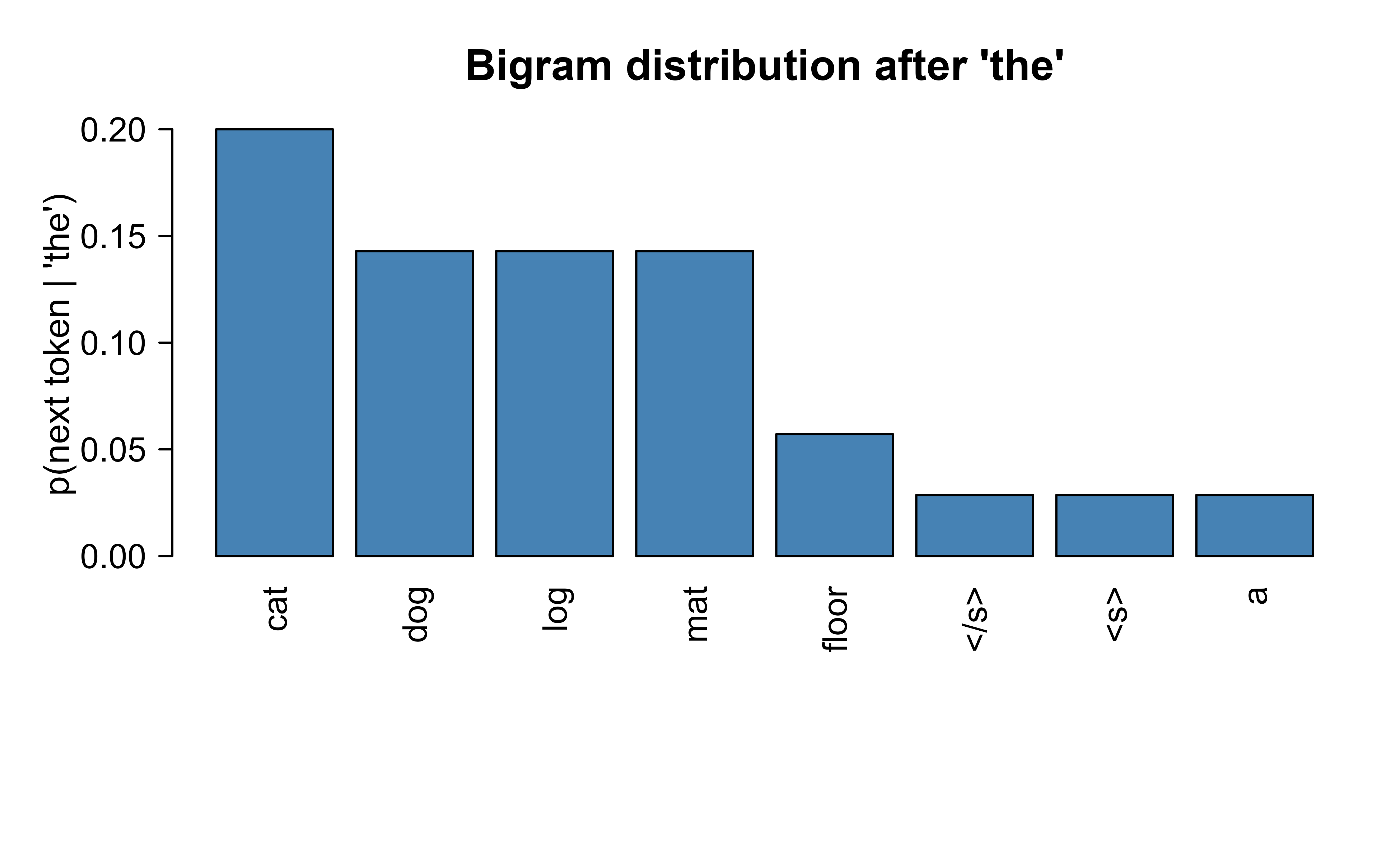
Table 40.1 lists the eight most probable continuations of the context word “the” under the smoothed bigram model.

# Top next-token probabilities for the context "the" under the bigram model.
context_word <- "the"
next_probs <- sapply(vocab, function(w)
  ngram_prob(bigram_model, context_word, w, V))
next_probs <- sort(next_probs, decreasing = TRUE)

top_table <- data.frame(
  next_token  = names(next_probs),
  probability = round(as.numeric(next_probs), 4),
  row.names   = NULL
)
knitr::kable(
  head(top_table, 8),
  caption = "Top eight bigram continuations of the context word 'the' with their smoothed conditional probabilities."
)

Table 40.1: Top eight bigram continuations of the context word ‘the’ with their smoothed conditional probabilities.

next_token	probability
cat	0.2000
dog	0.1429
log	0.1429
mat	0.1429
floor	0.0571
	0.0286
	0.0286
a	0.0286

Figure 40.1 shows the smoothed bigram distribution over the eight most likely continuations of the context word “the”, the same conditional next-token estimate that every step below reuses.

top8 <- head(top_table, 8)
op <- par(mar = c(7, 4, 3, 1))
barplot(
  height    = top8$probability,
  names.arg = top8$next_token,
  las       = 2,
  col       = "steelblue",
  ylab      = "p(next token | 'the')",
  main      = "Bigram distribution after 'the'"
)
par(op)

Figure 40.1: Bigram conditional next-token distribution given the context word ‘the’ (top 8 continuations).

# Generate text by sampling one token at a time from the bigram model,
# starting at the BOS marker and stopping at EOS or a length cap.
generate_text <- function(model, vocab, vocab_size, max_len = 15) {
  sentence <- c(BOS)
  for (i in seq_len(max_len)) {
    context <- sentence[length(sentence)]
    probs   <- sapply(vocab, function(w)
      ngram_prob(model, context, w, vocab_size))
    probs   <- probs / sum(probs)
    nxt     <- sample(vocab, size = 1, prob = probs)
    if (nxt == EOS) break
    sentence <- c(sentence, nxt)
  }
  paste(sentence[sentence != BOS & sentence != EOS], collapse = " ")
}

generated <- replicate(3, generate_text(bigram_model, vocab, V))
generated
#> [1] "the on cat to was on and was log floor a on mat"
#> [2] "to log"                                         
#> [3] "the to ran and"

Table 40.2 reports the held-out perplexity of the three models, and the same numbers are drawn as bars in the figure that follows.

# Perplexity on held-out text: exp of the average negative log-likelihood,
# exactly the definition from the start of the chapter.
perplexity <- function(model, n, test_lists, vocab_size) {
  total_logprob <- 0
  total_tokens  <- 0
  for (toks in test_lists) {
    if (length(toks) < n) next
    for (i in seq_len(length(toks) - n + 1)) {
      gram    <- toks[i:(i + n - 1)]
      context <- gram[-n]
      word    <- gram[n]
      p       <- ngram_prob(model, context, word, vocab_size)
      total_logprob <- total_logprob + log(p)
      total_tokens  <- total_tokens + 1
    }
  }
  exp(-total_logprob / total_tokens)
}

test_tokens <- lapply(test_corpus, tokenize)

ppl_bigram  <- perplexity(bigram_model,  2, test_tokens, V)
ppl_trigram <- perplexity(trigram_model, 3, test_tokens, V)

# A unigram baseline: ignore context entirely and use smoothed token frequencies.
unigram_counts <- table(unlist(train_tokens))
unigram_prob <- function(word, vocab_size) {
  c_w <- if (is.na(unigram_counts[word])) 0 else unigram_counts[word]
  (c_w + 1) / (sum(unigram_counts) + vocab_size)
}
ppl_unigram <- {
  lp <- 0; nt <- 0
  for (toks in test_tokens) {
    body <- toks[toks != BOS]
    for (w in body) { lp <- lp + log(unigram_prob(w, V)); nt <- nt + 1 }
  }
  exp(-lp / nt)
}

knitr::kable(
  data.frame(
    model      = c("unigram", "bigram", "trigram"),
    perplexity = round(c(ppl_unigram, ppl_bigram, ppl_trigram), 3)
  ),
  caption = "Held-out perplexity of the unigram, bigram, and trigram models on the test corpus."
)

Table 40.2: Held-out perplexity of the unigram, bigram, and trigram models on the test corpus.

model	perplexity
unigram	13.337
bigram	5.699
trigram	7.670

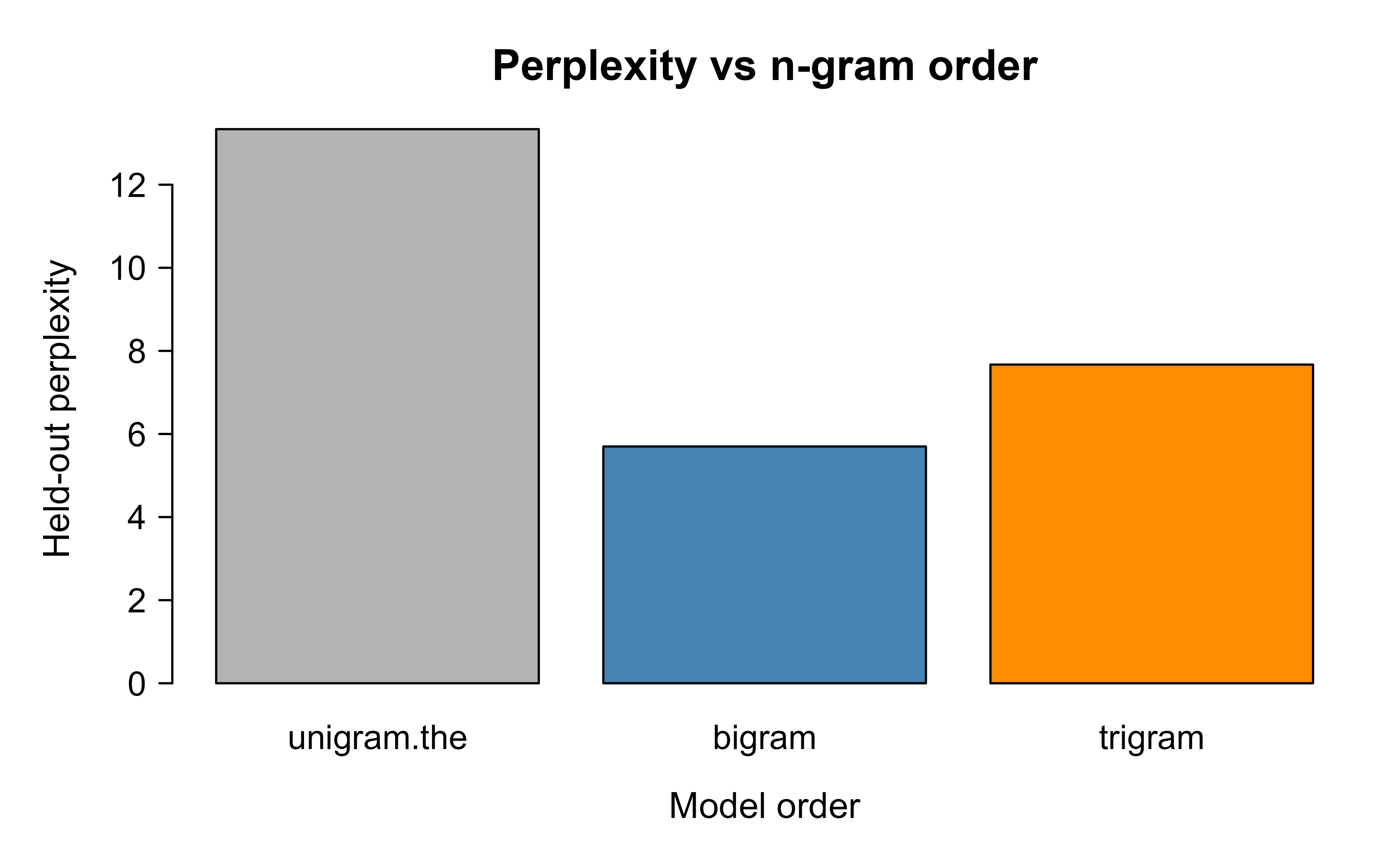
Figure 40.2 compares held-out perplexity across the unigram, bigram, and trigram models, making the effect of conditioning on more context visible at a glance.

ppl_vals <- c(unigram = ppl_unigram, bigram = ppl_bigram, trigram = ppl_trigram)
op <- par(mar = c(4, 4, 3, 1))
barplot(
  height    = ppl_vals,
  col       = c("grey70", "steelblue", "darkorange"),
  ylab      = "Held-out perplexity",
  xlab      = "Model order",
  main      = "Perplexity vs n-gram order"
)
par(op)

Figure 40.2: Held-out perplexity decreases as the n-gram order increases on this small corpus. Lower perplexity means the model is less surprised by the held-out text.

The pattern is the one to remember. Conditioning on more context (moving from unigram to bigram to trigram) lowers perplexity because the model is less surprised by real text, which is exactly the signal that drives the much larger neural and Transformer models in the rest of this part of the book. The only things that change at scale are how the conditional distribution \(p(x_t \mid x_{<t})\) is parameterized and how much data and compute go into estimating it.

40.7 Code You Would Run with Real Models

The base R demo above is for understanding. In practice you would call a pretrained model through a library. The snippets below are not executed here,⁶ but they show the shape of the workflow. Notice that the quantities are the same ones we defined by hand: the library returns a cross-entropy loss, and perplexity is just exp(loss).

# Scoring text and generating with a pretrained Transformer decoder (Python).
from transformers import AutoTokenizer, AutoModelForCausalLM
import torch

tokenizer = AutoTokenizer.from_pretrained("gpt2")
model = AutoModelForCausalLM.from_pretrained("gpt2")

text = "The cat sat on the"
inputs = tokenizer(text, return_tensors="pt")

with torch.no_grad():
    out = model(**inputs, labels=inputs["input_ids"])

# Cross-entropy loss, then perplexity = exp(loss), the same definition used above.
loss = out.loss.item()
perplexity = torch.exp(out.loss).item()

# Greedy continuation.
generated = model.generate(**inputs, max_new_tokens=10)
print(tokenizer.decode(generated[0]))

# A parameter-efficient fine-tuning sketch (conceptual, Python via reticulate
# or run directly in Python). LoRA freezes the base weights and learns small
# low-rank updates, so only a tiny fraction of parameters are trained.
# from peft import LoraConfig, get_peft_model
# config = LoraConfig(r = 8, lora_alpha = 16, target_modules = c("q_proj", "v_proj"))
# model  = get_peft_model(base_model, config)
# Train `model` on your labeled task as usual; only the adapters update.

40.8 Further Reading

• Vaswani, A., Shazeer, N., Parmar, N., Uszkoreit, J., Jones, L., Gomez, A. N., Kaiser, L., and Polosukhin, I. (2017). Attention Is All You Need. Advances in Neural Information Processing Systems.
• Brown, T. B., et al. (2020). Language Models Are Few-Shot Learners (GPT-3). Advances in Neural Information Processing Systems.
• Kaplan, J., McCandlish, S., Henighan, T., Brown, T. B., Chess, B., Child, R., Gray, S., Radford, A., Wu, J., and Amodei, D. (2020). Scaling Laws for Neural Language Models. arXiv preprint.
• Hoffmann, J., et al. (2022). Training Compute-Optimal Large Language Models (Chinchilla). Advances in Neural Information Processing Systems.
• Ouyang, L., et al. (2022). Training Language Models to Follow Instructions with Human Feedback (InstructGPT). Advances in Neural Information Processing Systems.

---

1. A token is the unit a model reads and predicts. For now you can think of it as roughly a word; the section on tokenization below explains why real models use subword pieces instead.

2. Negative log-likelihood is the same loss you have seen for logistic regression and softmax classifiers elsewhere in the book. A language model is, at each position, a classifier over the vocabulary, so it inherits exactly that objective.

3. Without smoothing, a single unseen continuation makes the sequence probability zero and the perplexity infinite. Add-one smoothing pretends every continuation was seen one extra time, which guarantees nonzero probabilities everywhere.

4. A power law means the loss falls by a roughly constant fraction each time you multiply a resource by a constant factor. Plotted on log-log axes it looks like a straight line, which is what makes extrapolation feasible.

5. Because no weights change, prompting is the cheapest thing to try first. Its main cost is that small changes in wording, example order, or formatting can swing results, so prompts deserve the same careful evaluation as any other modeling choice.

6. They require the Python transformers and peft packages plus a downloaded model and a deep-learning backend, none of which are part of this book’s build, so they are marked eval = FALSE.