A data analysis is rarely a single script run once. It is a graph of steps: read raw data, clean it, build features, fit several models, score them, and render a report. When one step changes, only the steps that depend on it need to rerun. Rerunning everything wastes time and, worse, invites the silent error where some outputs reflect old code and others reflect new code. The targets package brings the discipline of build systems such as make to R, so that a pipeline reruns exactly the steps that are out of date and skips the rest, while guaranteeing that the final outputs are consistent with the current code and data.
By the end of this chapter you will be able to think of an analysis as a dependency graph, decide when a step is genuinely out of date, write a targets pipeline that rebuilds only what changed, scale it across many inputs with branching, and run it in parallel. We start with intuition, then make the rebuild rule precise with a little notation, then show both a real targets pipeline and a tiny base R engine that demonstrates the same mechanism on code you can run yourself.
Intuition
Think of a recipe. If you change the frosting, you re-frost the cake; you do not re-bake it. A pipeline tool figures out the equivalent of “re-frost, do not re-bake” automatically, for every step, every time.
Because targets is probably not installed in your environment, the targets specific chunks are marked eval=FALSE. They are written to be correct and current so you can paste them into a session that has targets installed. To teach the core idea with code that actually runs, the chapter includes a base R pipeline engine that tracks dependencies with content hashes1 and skips up to date steps, which is the same mechanism targets uses under the hood.
103.1 Where this fits in a modern workflow
In a small project you might keep one long script. As the project grows, the script becomes slow to rerun and fragile: you comment out the expensive model fit while you tweak a plot, then forget to uncomment it, and the report is built from stale objects. A pipeline tool removes this hazard by making the dependency structure explicit and by deciding, automatically, what must run.
The idea is borrowed from software build systems. make reads a set of rules of the form “target \(T\) depends on prerequisites \(P_1, \dots, P_k\) and is produced by command \(C\).” It rebuilds \(T\) only when \(T\) is missing or older than some prerequisite. targets adapts this to R by representing each step as a target object, tracking dependencies between R objects rather than files, and deciding staleness by comparing content hashes rather than file timestamps. The result is a workflow that is incremental (only stale steps run), reproducible (outputs always match current code and data), and inspectable (you can draw the dependency graph).
In an ML or AI engineering setting this matters because the expensive steps, fitting a gradient boosting model (Chapter 12), computing embeddings (Chapter 110), running a cross validated tuning grid (Chapter 84), are exactly the ones you do not want to repeat unnecessarily. A pipeline lets you change a plot label and rebuild in seconds, while still guaranteeing that if you change the feature engineering, every downstream model and metric refits.
When to use this
Reach for a pipeline tool once an end to end rerun is slow enough to break your concentration, or once you have lost confidence that the report on disk reflects the current code. Below that threshold, a single tidy script is fine.
103.2 The dependency graph
To reason about “what depends on what,” we need one piece of vocabulary. Model a pipeline as a directed acyclic graph (DAG) \(G = (V, E)\).2 Each node \(v \in V\) is a target: a named result computed by some R expression. A directed edge \((u, v) \in E\) means that computing \(v\) uses the value of \(u\), so \(v\) depends on \(u\). Acyclicity is required: a cycle would mean a target depends on itself, directly or transitively, which has no well defined build order.
Because \(G\) is a DAG it admits a topological order, a sequence of the nodes in which every edge points forward. Build systems execute targets in a topological order so that each target’s inputs are ready before it runs. Independent targets, those with no path between them, can run in any order relative to each other, which is what allows parallel execution.
103.2.1 When does a target need to rebuild?
Assign to each target \(v\) a signature \(s(v)\) that summarizes everything the target’s value depends on: the code of its command, the values (or signatures) of its upstream dependencies, and any external files it reads. A common choice for the signature is a hash, a function \(h\) that maps arbitrary content to a fixed length digest such that different content almost surely yields different digests. Let \(\mathrm{cmd}(v)\) be the source of the command, \(\mathrm{deps}(v)\) the set of upstream targets, and \(\mathrm{files}(v)\) the external files. Then
\[
s(v) = h\Big( \mathrm{cmd}(v),\; \{\, s(u) : u \in \mathrm{deps}(v) \,\},\; \{\, h(\text{contents of } f) : f \in \mathrm{files}(v) \,\} \Big).
\]
The pipeline stores \(s(v)\) from the last successful run. On the next run it recomputes \(s(v)\) and rebuilds \(v\) if and only if the new signature differs from the stored one (or no stored value exists). Because each signature folds in the signatures of its dependencies, a change anywhere upstream propagates downstream: if you edit the code of target \(u\), then \(s(u)\) changes, which changes \(s(v)\) for every \(v\) that depends on \(u\), and the whole affected subgraph rebuilds while everything else is skipped.
Key idea
The signature folds in the signatures of its dependencies. That single recursive choice is what makes a change “ripple downstream” automatically: nothing has to track the ripple by hand, because the arithmetic of the hashes does it for you.
Two designs for the signature are worth distinguishing, and they differ in what question they ask about a target’s inputs.
Timestamps ask whether a target is older than any prerequisite. This is what make uses on files. It is cheap but fragile: touching a file without changing its contents forces a rebuild, and a clock skew across machines can give wrong answers.
Content hashes ask whether the actual contents changed. This is what targets uses. It is robust to timestamp noise and to moving files between machines, at the cost of reading and hashing content.
Warning
Timestamps lie in two directions. A file can be newer than its output yet have identical contents (a needless rebuild), or, after a clumsy file copy, be older than its output despite having changed (a missed rebuild). Content hashes avoid both failure modes, which is why modern tools prefer them.
The demo later in the chapter uses content hashing so the difference is concrete and runnable.
103.3 The targets package and the _targets.R script
With the rebuild rule in hand, we can look at how a real pipeline is written. A targets pipeline is defined in a single file named _targets.R at the project root. It loads the package, sources your functions, sets options (such as which packages each target needs), and returns a list of target objects built with tar_target(). Each tar_target(name, expression) declares a node: name is the target’s name and expression is the R code that produces it. The edges are not something you write down. targets discovers them automatically by static analysis of the expressions: if the expression for model mentions the symbol features, then model depends on features. You do not draw the graph by hand.
Note
Inferring edges from code is what keeps the graph honest. A hand maintained list of dependencies drifts out of date the moment someone edits a function and forgets to update the list. Reading the dependencies straight from the code means the graph cannot disagree with what the code actually does.
Show code
# _targets.R (lives at the project root)library(targets)# Functions used by the pipeline, kept in a separate filesource("R/functions.R")# Declare packages that targets should load when running each targettar_option_set(packages =c("dplyr", "ggplot2", "glmnet"))# The pipeline is a list of targets. Edges are inferred from the code:# clean uses raw_file, features uses clean, model uses features, etc.list(# An external file target: targets hashes the file's contentstar_target(raw_file, "data/raw.csv", format ="file"),tar_target(clean, read_and_clean(raw_file)),tar_target(features, build_features(clean)),tar_target(model, fit_model(features)),tar_target(metrics, evaluate(model, features)),tar_target(plot, plot_metrics(metrics)))
The functions referenced above live in R/functions.R, which keeps the pipeline file a thin declaration of structure and puts the real work in testable functions.
Show code
# R/functions.Rread_and_clean<-function(path){df<-read.csv(path)df[complete.cases(df), ]}build_features<-function(df){df$logx<-log1p(df$x)df}fit_model<-function(df){glmnet::cv.glmnet(as.matrix(df[, c("x", "logx")]), df$y, alpha =1)}evaluate<-function(model, df){pred<-as.numeric(predict(model, as.matrix(df[, c("x", "logx")]), s ="lambda.min"))data.frame(rmse =sqrt(mean((df$y-pred)^2)))}plot_metrics<-function(metrics){ggplot2::ggplot(metrics, ggplot2::aes(x ="model", y =rmse))+ggplot2::geom_col()}
Keeping the logic in R/functions.R and the structure in _targets.R is a deliberate split: the functions are ordinary R that you can test in isolation, and the pipeline file stays short enough to read at a glance.
Once the pipeline is declared, you drive it from the R console. The common verbs are these.
Show code
library(targets)tar_manifest()# list the declared targets and their commandstar_visnetwork()# draw the dependency graph, colored by up-to-date statustar_make()# build everything that is out of date, skip the resttar_read(metrics)# load a finished target's value into the sessiontar_load(c(model, metrics))# load several targets by nametar_outdated()# which targets would run on the next tar_make()
The first tar_make() runs every target and records each signature. If you then change only plot_metrics(), the next tar_make() reports that clean, features, model, and metrics are skipped and only plot runs. If instead you change build_features(), then features and everything downstream of it rebuilds, while clean is skipped. This is the staleness rule of the previous section in action.
Tip
Run tar_visnetwork() before tar_make(). It draws the graph with each node colored by whether it is up to date, so you can confirm that the dependencies you intended are the ones targets inferred, and see exactly what the next build will touch, before spending any compute.
103.4 A runnable base R pipeline that skips up-to-date steps
Reading about hashes and signatures is one thing; watching them skip steps is another. The following chunk runs. It implements a tiny pipeline engine in base R that does what targets does: it stores a signature for each step, and on rerun it executes a step only if its code or any upstream signature changed. The signature of a step folds in the hashes of its dependencies, so a change propagates downstream automatically.
Note
This engine is a teaching model, not a replacement for targets. It keeps everything in memory, hashes deparsed code rather than using a cryptographic digest, and ignores parallelism. The point is to make the rebuild rule tangible in code you can step through, not to ship a build system.
Show code
set.seed(1)# A content hash. We use a simple, deterministic digest of the# deparsed object so the demo needs no external package. A real# pipeline would use a cryptographic hash; the design idea is the same.hash<-function(x){s<-paste(deparse(x), collapse ="\n")bytes<-as.integer(charToRaw(s))# Polynomial rolling hash kept inside 32-bit signed integer range.# Reducing modulo a prime below 2^31 after every step avoids overflow,# so different content reliably yields different digests.modulus<-2147483647# 2^31 - 1, a Mersenne primebase<-16777619h<-2166136261%%modulusfor(binbytes){h<-(h*base+b)%%modulus}sprintf("%08x", as.integer(h))}# A "store" of signatures and cached values from the last buildstore<-new.env()# Define a target: a name, the names of its dependencies, and a# function of the dependency values that produces the target value.make_target<-function(name, deps, fun){list(name =name, deps =deps, fun =fun)}# The build engine. Given targets in dependency order, build each# only if its signature changed since the last run.build<-function(targets, verbose=TRUE){ran<-character(0)for(tgintargets){dep_sigs<-vapply(tg$deps, function(d)store[[paste0("sig_", d)]],character(1))# Signature folds in the code of the command and the signatures# of all upstream dependencies (see the staleness formula).sig<-hash(list(body =body(tg$fun), deps =dep_sigs))stored<-store[[paste0("sig_", tg$name)]]if(is.null(stored)||!identical(stored, sig)){dep_vals<-lapply(tg$deps, function(d)store[[paste0("val_", d)]])val<-do.call(tg$fun, dep_vals)store[[paste0("val_", tg$name)]]<-valstore[[paste0("sig_", tg$name)]]<-sigran<-c(ran, tg$name)if(verbose)message("RUN ", tg$name)}else{if(verbose)message("skip ", tg$name)}}invisible(ran)}# Define a four-step pipeline. The functions mimic real work.pipeline<-list(make_target("clean", character(0), function(){Sys.sleep(0)# pretend this reads and cleans datadata.frame(x =1:200, y =2*(1:200)+rnorm(200, sd =10))}),make_target("features", "clean", function(clean){clean$logx<-log(clean$x)clean}),make_target("model", "features", function(features){lm(y~x+logx, data =features)# the "expensive" step}),make_target("metrics", "model", function(model){data.frame(rmse =sqrt(mean(residuals(model)^2)))}))cat("First build (everything is new):\n")#> First build (everything is new):first<-build(pipeline)cat("\nSecond build with no changes (everything is up to date):\n")#> #> Second build with no changes (everything is up to date):second<-build(pipeline)cat("\nTargets that ran on the first build: ", paste(first, collapse =", "),"\nTargets that ran on the second build:",if(length(second))paste(second, collapse =", ")else"(none)", "\n")#> #> Targets that ran on the first build: clean, features, model, metrics #> Targets that ran on the second build: (none)
The second build runs nothing because no signature changed. Now change one upstream step and rebuild. Editing the features command changes its signature, which changes the signature of model and then metrics, so those three rebuild while clean is skipped.
Show code
# Edit the "features" step: add a squared term. Only this step and# everything downstream of it should rerun; "clean" should be skipped.pipeline[[2]]<-make_target("features", "clean", function(clean){clean$logx<-log(clean$x)clean$x2<-clean$x^2# the changeclean})cat("Build after editing the 'features' step:\n")#> Build after editing the 'features' step:changed<-build(pipeline)cat("\nTargets that reran:", paste(changed, collapse =", "), "\n")#> #> Targets that reran: features, model, metrics
This is the entire value proposition in miniature: a one line change to feature engineering reruns only the affected subgraph, and an unrelated change (say, to a downstream plot) would never trigger the model to refit. targets does the same thing, just with a robust hash, a persistent on disk store, automatic edge detection, and parallelism, all of which we get to next.
103.4.1 A figure: cost of full reruns versus incremental builds
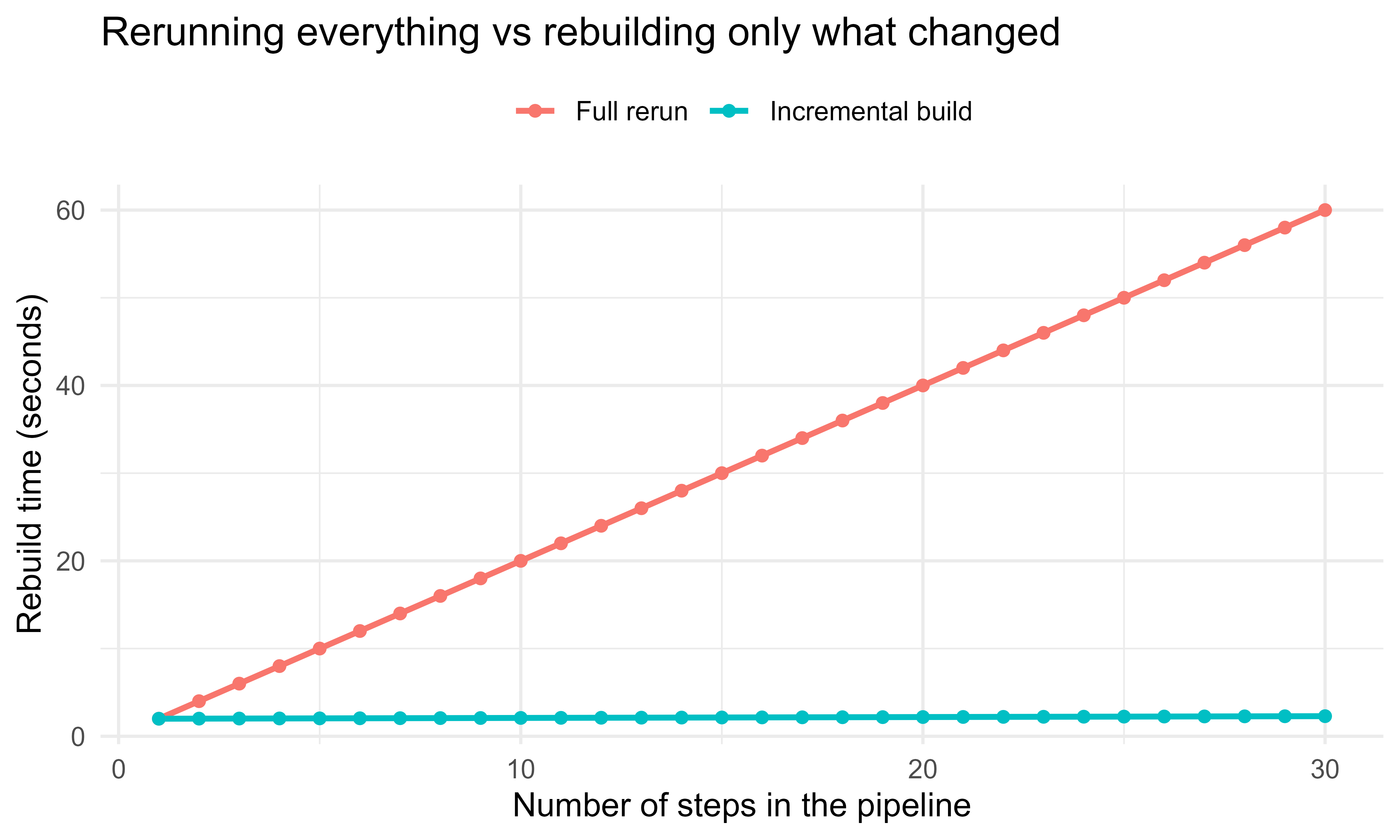
The payoff grows with pipeline length and with how expensive the unchanged steps are. Suppose a pipeline has \(n\) steps in a chain, each costing \(c\) seconds, and you edit only the last step. A naive rerun costs \(n c\). An incremental build reruns only the edited step (and its descendants, here just one step), costing \(c\) plus a small hashing overhead \(\epsilon\) per skipped step. Figure 103.1 plots the two costs as the chain grows.
Show code
library(ggplot2)c_step<-2.0# seconds per step if it runsepsilon<-0.01# seconds to hash and skip an up-to-date stepn_steps<-1:30full_rerun<-n_steps*c_stepincremental<-c_step+(n_steps-1)*epsilon# only the last step runsdf<-rbind(data.frame(n =n_steps, seconds =full_rerun, strategy ="Full rerun"),data.frame(n =n_steps, seconds =incremental, strategy ="Incremental build"))ggplot(df, aes(x =n, y =seconds, colour =strategy))+geom_line(linewidth =1)+geom_point(size =1.6)+labs(x ="Number of steps in the pipeline", y ="Rebuild time (seconds)", colour =NULL, title ="Rerunning everything vs rebuilding only what changed")+theme_minimal(base_size =12)+theme(legend.position ="top")
Figure 103.1: Wall-clock cost of rebuilding a chain pipeline when only the last step changes. Full rerun grows linearly with the number of steps; the incremental build stays nearly flat because skipped steps cost only a hash check.
The gap between the lines is the time targets saves you on every edit that does not touch the expensive upstream steps. In a real project where one step is a multi minute model fit, this is the difference between an interactive loop and a coffee break.
103.5 Branching: one target, many values
So far each target has produced one value. Often, though, you want to apply the same computation across many inputs: fit the same model to each of fifty files, or sweep a hyperparameter over a grid, or bootstrap a statistic across many resamples. Writing one target per input by hand does not scale, and it loses the incremental benefit, since editing one input should not rerun the other forty nine. targets solves this with branching, which creates many sub targets from a pattern over upstream targets.
Two flavors exist, and the choice between them comes down to when you know the inputs.
Static branching with tar_map() expands the pattern at the time you write the pipeline, producing named branches you can see in the manifest. Use it when the set of inputs is fixed and known in advance.
Dynamic branching with the pattern argument creates branches at run time from the length of an upstream target. Use it when the number of inputs is not known until the pipeline runs, for example one branch per file found in a directory.
Show code
library(targets)library(tarchetypes)# provides tar_map() and helperslist(# An upstream target that lists the inputs to branch overtar_target(files, list.files("data", full.names =TRUE)),# Dynamic branching: one branch per element of `files`.# map() runs the command once per file; targets tracks each branch.tar_target(cleaned,read_and_clean(files), pattern =map(files)),# cross() forms the Cartesian product: every model type on every filetar_target(model_types, c("lasso", "ridge")),tar_target(fits,fit_one(cleaned, model_types), pattern =cross(cleaned, model_types)),# A reduce-style target that combines all branch results into one tabletar_target(summary, dplyr::bind_rows(fits)))
The mathematics of branching is just an index set. If files has elements indexed by \(i \in \{1, \dots, m\}\) and model_types by \(j \in \{1, \dots, r\}\), then map(files) produces targets indexed by \(i\), and cross(cleaned, model_types) produces targets indexed by the product set \(\{(i, j)\}\), of size \(m r\). Each branch has its own signature, so editing one input file rebuilds only the branches that read it, not the whole sweep.
Warning
cross() multiplies. Two factors give \(m r\) branches; a third gives \(m r s\), and so on. A cross of three modest grids can quietly produce thousands of branches, each with its own metadata to track. Use cross() only over the dimensions you genuinely need to vary together.
103.6 Scaling: parallel and distributed builds
Branching does more than save typing: by creating many independent targets, it gives the build something to parallelize. Independent targets, those with no path between them in \(G\), can run at the same time, applying the ideas from the parallel computing chapter (Chapter 95) to the pipeline as a whole. targets delegates this to the crew package, which manages a pool of worker processes (local or on a cluster or cloud). You change how the pipeline scales without changing what it computes: the targets and their edges stay the same, only the controller changes.
Show code
# In _targets.R, add a controller for parallel local workerslibrary(targets)library(crew)tar_option_set( controller =crew_controller_local(workers =4))# Then build as usual; independent targets and branches run on the pool# tar_make() uses the controller automatically
The speedup is bounded by the structure of the graph, not just the number of workers. If the longest dependency chain (the critical path) has total cost \(T_\infty\) and the total work across all targets is \(T_1\), then with \(p\) workers the build time obeys
No amount of parallelism beats the critical path \(T_\infty\), because each step on it must wait for its predecessor. Branching helps precisely because it creates many independent targets, widening the graph so more work can proceed in parallel and \(T_1 / p\) becomes the binding term rather than \(T_\infty\).
Intuition
A deep, narrow pipeline (one long chain) cannot be sped up much by adding workers, because every step waits on the one before it. A wide pipeline (many independent branches) can. If parallelism is not helping, the graph is probably too chain like, and the cure is to find work that can be split into independent branches.
103.7 Comparison: targets, drake, make, and a plain script
targets is the current successor to drake, which pioneered hash based pipelines in R. drake is no longer actively developed and its author recommends targets for new projects. Table 103.1 contrasts the four approaches on the points that matter in practice.
Table 103.1: Comparison of a plain R script, GNU make, drake, and targets across the workflow properties that matter in practice.
Property
Plain R script
GNU make
drake
targets
Unit of work
lines of code
file targets
R objects
R objects
Staleness test
none (always reruns all)
file timestamps
content hash
content hash
Dependency edges
implicit, in your head
written by hand in Makefile
inferred from code
inferred from code
Skips up-to-date steps
no
yes
yes
yes
Stores results
you manage .RData by hand
files on disk
hidden cache
_targets/ object store
Branching over inputs
manual loops
manual rules
map/cross plans
map/cross + tar_map()
Parallel backend
manual (future, parallel)
make -j
future, clustermq
crew (local, cluster, cloud)
Visualize the graph
no
external tools
vis_drake_graph()
tar_visnetwork()
Status
works, error prone
language agnostic, R unaware
superseded, maintenance only
actively developed, recommended
The honest summary: a plain script is fine until reruns get slow or the object bookkeeping gets error prone. make is excellent and language agnostic but knows nothing about R objects, so you must marshal everything through files and hand write the rules. drake solved the R specific problem first; targets is its cleaner redesign with a smaller, more predictable internal model and the modern crew backend, and it is what you should reach for today.
103.8 Practical guidance, pitfalls, and when to use it
Use targets when reruns have become slow enough to disrupt your iteration loop, when you have expensive steps you do not want to repeat, when a project has enough steps that you have lost track of what depends on what, or when you need a pipeline that a collaborator (or future you) can rebuild from scratch with one command and trust the result. It pairs naturally with R Markdown or Quarto reports as a final target, so the rendered document is always built from current upstream results.
Most of the trouble people hit comes from a handful of recurring mistakes. The common pitfalls are these.
Hidden side effects. targets tracks values, not side effects. If a target writes to a database or downloads a file as a side effect and returns nothing meaningful, the dependency tracking cannot see it. Make external files explicit format = "file" targets so their contents are hashed, and return the path from the target.
Global state and randomness. A target that depends on a global option, an environment variable, or an unset random seed can produce different results without its signature changing. Pass such inputs in as dependencies, and set seeds explicitly (targets manages per target seeds for you, but reproducibility still requires that your functions be deterministic given their inputs).
Giant monolithic targets. If one target does everything, you lose the benefit of incremental rebuilds, because any change reruns the whole thing. Split work into the natural steps so that an edit reruns only the affected part.
Functions defined in _targets.R instead of sourced files. Keep real logic in R/ files that are sourced, and keep _targets.R a thin list of tar_target() calls. This keeps functions testable on their own and keeps the pipeline file readable.
Branch explosion. cross() over several factors multiplies branch counts (\(m r\) in the earlier notation, and more with additional factors). A cross of three modest grids can produce thousands of branches and a slow metadata bookkeeping step. Branch only over what you truly need to vary.
Confusing the object store with version control. The _targets/ directory is a cache, not source. Commit _targets.R and your R/ functions to version control; the object store is regenerated by tar_make().
A reasonable default workflow is short. Write your real work as functions in R/, declare a thin _targets.R listing the steps, run tar_visnetwork() to sanity check the graph, run tar_make(), and iterate. When the input sweep grows, add branching. When the build gets slow and the graph is wide, add a crew controller. Treat the rendered report as the terminal target so it is never out of date with respect to the data and code.
To recap the chapter in one breath: model an analysis as a DAG, give each target a content based signature that folds in its dependencies, and rebuild a target exactly when its signature changes. That one rule buys incremental rebuilds, reproducibility, and an inspectable graph. targets implements it for R objects with automatic edge detection, branching for many inputs, and a crew backend for parallel and distributed builds. The runnable base R engine above is the same idea stripped to its essentials, so if you understood why it skipped the right steps, you understand targets.
103.9 Further reading
Landau (2021). “The targets R package: a dynamic Make-like function-oriented pipeline toolkit for reproducibility and high-performance computing.” Journal of Open Source Software.
Landau (2018). “The drake R package: a pipeline toolkit for reproducibility and high-performance computing.” Journal of Open Source Software. Background on the predecessor and the hash based design.
The targets user manual and the targets R Markdown/Quarto guides, maintained by Landau, for current API and patterns (_targets.R, dynamic and static branching, crew).
Stallman, McGrath, and Smith (2020). “GNU Make: A Program for Directing Recompilation.” Free Software Foundation. The original timestamp based build system that motivates the design.
Wilson, Bryan, Cranston, Kitzes, Nederbragt, and Teal (2017). “Good enough practices in scientific computing.” PLoS Computational Biology. For the broader case for reproducible, automated analysis pipelines.
A hash is a function that maps any input to a short, fixed length string of characters (its digest), with the property that even a one character change in the input produces a completely different digest. We define a small one in the runnable demo below.↩︎
Directed means each edge has a direction (from a dependency to the thing that uses it). Acyclic means you can never follow the arrows in a loop back to where you started. Graph is just the collection of nodes and edges.↩︎
Source Code
# Reproducible Pipelines with targets {#sec-reproducible-pipelines-targets}```{r}#| include: falsesource("_common.R")```A data analysis is rarely a single script run once. It is a graph of steps: read raw data, clean it, build features, fit several models, score them, and render a report. When one step changes, only the steps that depend on it need to rerun. Rerunning everything wastes time and, worse, invites the silent error where some outputs reflect old code and others reflect new code. The `targets` package brings the discipline of build systems such as `make` to R, so that a pipeline reruns exactly the steps that are out of date and skips the rest, while guaranteeing that the final outputs are consistent with the current code and data.By the end of this chapter you will be able to think of an analysis as a dependency graph, decide when a step is genuinely out of date, write a `targets` pipeline that rebuilds only what changed, scale it across many inputs with branching, and run it in parallel. We start with intuition, then make the rebuild rule precise with a little notation, then show both a real `targets` pipeline and a tiny base R engine that demonstrates the same mechanism on code you can run yourself.::: {.callout-tip title="Intuition"}Think of a recipe. If you change the frosting, you re-frost the cake; you do not re-bake it. A pipeline tool figures out the equivalent of "re-frost, do not re-bake" automatically, for every step, every time.:::Because `targets` is probably not installed in your environment, the `targets` specific chunks are marked `eval=FALSE`. They are written to be correct and current so you can paste them into a session that has `targets` installed. To teach the core idea with code that actually runs, the chapter includes a base R pipeline engine that tracks dependencies with content hashes^[A *hash* is a function that maps any input to a short, fixed length string of characters (its *digest*), with the property that even a one character change in the input produces a completely different digest. We define a small one in the runnable demo below.] and skips up to date steps, which is the same mechanism `targets` uses under the hood.## Where this fits in a modern workflowIn a small project you might keep one long script. As the project grows, the script becomes slow to rerun and fragile: you comment out the expensive model fit while you tweak a plot, then forget to uncomment it, and the report is built from stale objects. A pipeline tool removes this hazard by making the dependency structure explicit and by deciding, automatically, what must run.The idea is borrowed from software build systems. `make` reads a set of rules of the form "target $T$ depends on prerequisites $P_1, \dots, P_k$ and is produced by command $C$." It rebuilds $T$ only when $T$ is missing or older than some prerequisite. `targets` adapts this to R by representing each step as a target object, tracking dependencies between R objects rather than files, and deciding staleness by comparing content hashes rather than file timestamps. The result is a workflow that is incremental (only stale steps run), reproducible (outputs always match current code and data), and inspectable (you can draw the dependency graph).In an ML or AI engineering setting this matters because the expensive steps, fitting a gradient boosting model (@sec-gradient-boosting), computing embeddings (@sec-embeddings-vector-search), running a cross validated tuning grid (@sec-hyperparameter-optimization), are exactly the ones you do not want to repeat unnecessarily. A pipeline lets you change a plot label and rebuild in seconds, while still guaranteeing that if you change the feature engineering, every downstream model and metric refits.::: {.callout-tip title="When to use this"}Reach for a pipeline tool once an end to end rerun is slow enough to break your concentration, or once you have lost confidence that the report on disk reflects the current code. Below that threshold, a single tidy script is fine.:::## The dependency graphTo reason about "what depends on what," we need one piece of vocabulary. Model a pipeline as a directed acyclic graph (DAG) $G = (V, E)$.^[*Directed* means each edge has a direction (from a dependency to the thing that uses it). *Acyclic* means you can never follow the arrows in a loop back to where you started. *Graph* is just the collection of nodes and edges.] Each node $v \in V$ is a target: a named result computed by some R expression. A directed edge $(u, v) \in E$ means that computing $v$ uses the value of $u$, so $v$ depends on $u$. Acyclicity is required: a cycle would mean a target depends on itself, directly or transitively, which has no well defined build order.Because $G$ is a DAG it admits a topological order, a sequence of the nodes in which every edge points forward. Build systems execute targets in a topological order so that each target's inputs are ready before it runs. Independent targets, those with no path between them, can run in any order relative to each other, which is what allows parallel execution.### When does a target need to rebuild?Assign to each target $v$ a signature $s(v)$ that summarizes everything the target's value depends on: the code of its command, the values (or signatures) of its upstream dependencies, and any external files it reads. A common choice for the signature is a hash, a function $h$ that maps arbitrary content to a fixed length digest such that different content almost surely yields different digests. Let $\mathrm{cmd}(v)$ be the source of the command, $\mathrm{deps}(v)$ the set of upstream targets, and $\mathrm{files}(v)$ the external files. Then$$s(v) = h\Big( \mathrm{cmd}(v),\; \{\, s(u) : u \in \mathrm{deps}(v) \,\},\; \{\, h(\text{contents of } f) : f \in \mathrm{files}(v) \,\} \Big).$$The pipeline stores $s(v)$ from the last successful run. On the next run it recomputes $s(v)$ and rebuilds $v$ if and only if the new signature differs from the stored one (or no stored value exists). Because each signature folds in the signatures of its dependencies, a change anywhere upstream propagates downstream: if you edit the code of target $u$, then $s(u)$ changes, which changes $s(v)$ for every $v$ that depends on $u$, and the whole affected subgraph rebuilds while everything else is skipped.::: {.callout-important title="Key idea"}The signature folds in the signatures of its dependencies. That single recursive choice is what makes a change "ripple downstream" automatically: nothing has to track the ripple by hand, because the arithmetic of the hashes does it for you.:::Two designs for the signature are worth distinguishing, and they differ in what question they ask about a target's inputs.- Timestamps ask whether a target is older than any prerequisite. This is what `make` uses on files. It is cheap but fragile: touching a file without changing its contents forces a rebuild, and a clock skew across machines can give wrong answers.- Content hashes ask whether the actual contents changed. This is what `targets` uses. It is robust to timestamp noise and to moving files between machines, at the cost of reading and hashing content.::: {.callout-warning}Timestamps lie in two directions. A file can be newer than its output yet have identical contents (a needless rebuild), or, after a clumsy file copy, be older than its output despite having changed (a missed rebuild). Content hashes avoid both failure modes, which is why modern tools prefer them.:::The demo later in the chapter uses content hashing so the difference is concrete and runnable.## The targets package and the `_targets.R` scriptWith the rebuild rule in hand, we can look at how a real pipeline is written. A `targets` pipeline is defined in a single file named `_targets.R` at the project root. It loads the package, sources your functions, sets options (such as which packages each target needs), and returns a list of target objects built with `tar_target()`. Each `tar_target(name, expression)` declares a node: `name` is the target's name and `expression` is the R code that produces it. The edges are not something you write down. `targets` discovers them automatically by static analysis of the expressions: if the expression for `model` mentions the symbol `features`, then `model` depends on `features`. You do not draw the graph by hand.::: {.callout-note}Inferring edges from code is what keeps the graph honest. A hand maintained list of dependencies drifts out of date the moment someone edits a function and forgets to update the list. Reading the dependencies straight from the code means the graph cannot disagree with what the code actually does.:::```{r targets-script, eval=FALSE}# _targets.R (lives at the project root)library(targets)# Functions used by the pipeline, kept in a separate filesource("R/functions.R")# Declare packages that targets should load when running each targettar_option_set(packages =c("dplyr", "ggplot2", "glmnet"))# The pipeline is a list of targets. Edges are inferred from the code:# clean uses raw_file, features uses clean, model uses features, etc.list(# An external file target: targets hashes the file's contentstar_target(raw_file, "data/raw.csv", format ="file"),tar_target(clean, read_and_clean(raw_file)),tar_target(features, build_features(clean)),tar_target(model, fit_model(features)),tar_target(metrics, evaluate(model, features)),tar_target(plot, plot_metrics(metrics)))```The functions referenced above live in `R/functions.R`, which keeps the pipeline file a thin declaration of structure and puts the real work in testable functions.```{r targets-functions, eval=FALSE}# R/functions.Rread_and_clean <-function(path) { df <-read.csv(path) df[complete.cases(df), ]}build_features <-function(df) { df$logx <-log1p(df$x) df}fit_model <-function(df) { glmnet::cv.glmnet(as.matrix(df[, c("x", "logx")]), df$y, alpha =1)}evaluate <-function(model, df) { pred <-as.numeric(predict(model, as.matrix(df[, c("x", "logx")]),s ="lambda.min"))data.frame(rmse =sqrt(mean((df$y - pred)^2)))}plot_metrics <-function(metrics) { ggplot2::ggplot(metrics, ggplot2::aes(x ="model", y = rmse)) + ggplot2::geom_col()}```Keeping the logic in `R/functions.R` and the structure in `_targets.R` is a deliberate split: the functions are ordinary R that you can test in isolation, and the pipeline file stays short enough to read at a glance.Once the pipeline is declared, you drive it from the R console. The common verbs are these.```{r targets-run, eval=FALSE}library(targets)tar_manifest() # list the declared targets and their commandstar_visnetwork() # draw the dependency graph, colored by up-to-date statustar_make() # build everything that is out of date, skip the resttar_read(metrics) # load a finished target's value into the sessiontar_load(c(model, metrics)) # load several targets by nametar_outdated() # which targets would run on the next tar_make()```The first `tar_make()` runs every target and records each signature. If you then change only `plot_metrics()`, the next `tar_make()` reports that `clean`, `features`, `model`, and `metrics` are skipped and only `plot` runs. If instead you change `build_features()`, then `features` and everything downstream of it rebuilds, while `clean` is skipped. This is the staleness rule of the previous section in action.::: {.callout-tip}Run `tar_visnetwork()` before `tar_make()`. It draws the graph with each node colored by whether it is up to date, so you can confirm that the dependencies you intended are the ones `targets` inferred, and see exactly what the next build will touch, before spending any compute.:::## A runnable base R pipeline that skips up-to-date stepsReading about hashes and signatures is one thing; watching them skip steps is another. The following chunk runs. It implements a tiny pipeline engine in base R that does what `targets` does: it stores a signature for each step, and on rerun it executes a step only if its code or any upstream signature changed. The signature of a step folds in the hashes of its dependencies, so a change propagates downstream automatically.::: {.callout-note}This engine is a teaching model, not a replacement for `targets`. It keeps everything in memory, hashes deparsed code rather than using a cryptographic digest, and ignores parallelism. The point is to make the rebuild rule tangible in code you can step through, not to ship a build system.:::```{r base-pipeline}set.seed(1)# A content hash. We use a simple, deterministic digest of the# deparsed object so the demo needs no external package. A real# pipeline would use a cryptographic hash; the design idea is the same.hash <-function(x) { s <-paste(deparse(x), collapse ="\n") bytes <-as.integer(charToRaw(s))# Polynomial rolling hash kept inside 32-bit signed integer range.# Reducing modulo a prime below 2^31 after every step avoids overflow,# so different content reliably yields different digests. modulus <-2147483647# 2^31 - 1, a Mersenne prime base <-16777619 h <-2166136261%% modulusfor (b in bytes) { h <- (h * base + b) %% modulus }sprintf("%08x", as.integer(h))}# A "store" of signatures and cached values from the last buildstore <-new.env()# Define a target: a name, the names of its dependencies, and a# function of the dependency values that produces the target value.make_target <-function(name, deps, fun) {list(name = name, deps = deps, fun = fun)}# The build engine. Given targets in dependency order, build each# only if its signature changed since the last run.build <-function(targets, verbose =TRUE) { ran <-character(0)for (tg in targets) { dep_sigs <-vapply(tg$deps, function(d) store[[paste0("sig_", d)]],character(1))# Signature folds in the code of the command and the signatures# of all upstream dependencies (see the staleness formula). sig <-hash(list(body =body(tg$fun), deps = dep_sigs)) stored <- store[[paste0("sig_", tg$name)]]if (is.null(stored) ||!identical(stored, sig)) { dep_vals <-lapply(tg$deps, function(d) store[[paste0("val_", d)]]) val <-do.call(tg$fun, dep_vals) store[[paste0("val_", tg$name)]] <- val store[[paste0("sig_", tg$name)]] <- sig ran <-c(ran, tg$name)if (verbose) message("RUN ", tg$name) } else {if (verbose) message("skip ", tg$name) } }invisible(ran)}# Define a four-step pipeline. The functions mimic real work.pipeline <-list(make_target("clean", character(0), function() {Sys.sleep(0) # pretend this reads and cleans datadata.frame(x =1:200, y =2* (1:200) +rnorm(200, sd =10)) }),make_target("features", "clean", function(clean) { clean$logx <-log(clean$x) clean }),make_target("model", "features", function(features) {lm(y ~ x + logx, data = features) # the "expensive" step }),make_target("metrics", "model", function(model) {data.frame(rmse =sqrt(mean(residuals(model)^2))) }))cat("First build (everything is new):\n")first <-build(pipeline)cat("\nSecond build with no changes (everything is up to date):\n")second <-build(pipeline)cat("\nTargets that ran on the first build: ", paste(first, collapse =", "),"\nTargets that ran on the second build:",if (length(second)) paste(second, collapse =", ") else"(none)", "\n")```The second build runs nothing because no signature changed. Now change one upstream step and rebuild. Editing the `features` command changes its signature, which changes the signature of `model` and then `metrics`, so those three rebuild while `clean` is skipped.```{r base-pipeline-change}# Edit the "features" step: add a squared term. Only this step and# everything downstream of it should rerun; "clean" should be skipped.pipeline[[2]] <-make_target("features", "clean", function(clean) { clean$logx <-log(clean$x) clean$x2 <- clean$x^2# the change clean})cat("Build after editing the 'features' step:\n")changed <-build(pipeline)cat("\nTargets that reran:", paste(changed, collapse =", "), "\n")```This is the entire value proposition in miniature: a one line change to feature engineering reruns only the affected subgraph, and an unrelated change (say, to a downstream plot) would never trigger the model to refit. `targets` does the same thing, just with a robust hash, a persistent on disk store, automatic edge detection, and parallelism, all of which we get to next.### A figure: cost of full reruns versus incremental buildsThe payoff grows with pipeline length and with how expensive the unchanged steps are. Suppose a pipeline has $n$ steps in a chain, each costing $c$ seconds, and you edit only the last step. A naive rerun costs $n c$. An incremental build reruns only the edited step (and its descendants, here just one step), costing $c$ plus a small hashing overhead $\epsilon$ per skipped step. @fig-reproducible-pipelines-targets-cost plots the two costs as the chain grows.```{r fig-reproducible-pipelines-targets-cost, fig.cap="Wall-clock cost of rebuilding a chain pipeline when only the last step changes. Full rerun grows linearly with the number of steps; the incremental build stays nearly flat because skipped steps cost only a hash check.", fig.width=7, fig.height=4.2}library(ggplot2)c_step <-2.0# seconds per step if it runsepsilon <-0.01# seconds to hash and skip an up-to-date stepn_steps <-1:30full_rerun <- n_steps * c_stepincremental <- c_step + (n_steps -1) * epsilon # only the last step runsdf <-rbind(data.frame(n = n_steps, seconds = full_rerun, strategy ="Full rerun"),data.frame(n = n_steps, seconds = incremental, strategy ="Incremental build"))ggplot(df, aes(x = n, y = seconds, colour = strategy)) +geom_line(linewidth =1) +geom_point(size =1.6) +labs(x ="Number of steps in the pipeline",y ="Rebuild time (seconds)",colour =NULL,title ="Rerunning everything vs rebuilding only what changed") +theme_minimal(base_size =12) +theme(legend.position ="top")```The gap between the lines is the time `targets` saves you on every edit that does not touch the expensive upstream steps. In a real project where one step is a multi minute model fit, this is the difference between an interactive loop and a coffee break.## Branching: one target, many valuesSo far each target has produced one value. Often, though, you want to apply the same computation across many inputs: fit the same model to each of fifty files, or sweep a hyperparameter over a grid, or bootstrap a statistic across many resamples. Writing one target per input by hand does not scale, and it loses the incremental benefit, since editing one input should not rerun the other forty nine. `targets` solves this with branching, which creates many sub targets from a pattern over upstream targets.Two flavors exist, and the choice between them comes down to when you know the inputs.- Static branching with `tar_map()` expands the pattern at the time you write the pipeline, producing named branches you can see in the manifest. Use it when the set of inputs is fixed and known in advance.- Dynamic branching with the `pattern` argument creates branches at run time from the length of an upstream target. Use it when the number of inputs is not known until the pipeline runs, for example one branch per file found in a directory.```{r targets-branching, eval=FALSE}library(targets)library(tarchetypes) # provides tar_map() and helperslist(# An upstream target that lists the inputs to branch overtar_target(files, list.files("data", full.names =TRUE)),# Dynamic branching: one branch per element of `files`.# map() runs the command once per file; targets tracks each branch.tar_target( cleaned,read_and_clean(files),pattern =map(files) ),# cross() forms the Cartesian product: every model type on every filetar_target(model_types, c("lasso", "ridge")),tar_target( fits,fit_one(cleaned, model_types),pattern =cross(cleaned, model_types) ),# A reduce-style target that combines all branch results into one tabletar_target(summary, dplyr::bind_rows(fits)))```The mathematics of branching is just an index set. If `files` has elements indexed by $i \in \{1, \dots, m\}$ and `model_types` by $j \in \{1, \dots, r\}$, then `map(files)` produces targets indexed by $i$, and `cross(cleaned, model_types)` produces targets indexed by the product set $\{(i, j)\}$, of size $m r$. Each branch has its own signature, so editing one input file rebuilds only the branches that read it, not the whole sweep.::: {.callout-warning}`cross()` multiplies. Two factors give $m r$ branches; a third gives $m r s$, and so on. A cross of three modest grids can quietly produce thousands of branches, each with its own metadata to track. Use `cross()` only over the dimensions you genuinely need to vary together.:::## Scaling: parallel and distributed buildsBranching does more than save typing: by creating many independent targets, it gives the build something to parallelize. Independent targets, those with no path between them in $G$, can run at the same time, applying the ideas from the parallel computing chapter (@sec-parallel-computing) to the pipeline as a whole. `targets` delegates this to the `crew` package, which manages a pool of worker processes (local or on a cluster or cloud). You change how the pipeline scales without changing what it computes: the targets and their edges stay the same, only the controller changes.```{r targets-parallel, eval=FALSE}# In _targets.R, add a controller for parallel local workerslibrary(targets)library(crew)tar_option_set(controller =crew_controller_local(workers =4))# Then build as usual; independent targets and branches run on the pool# tar_make() uses the controller automatically```The speedup is bounded by the structure of the graph, not just the number of workers. If the longest dependency chain (the critical path) has total cost $T_\infty$ and the total work across all targets is $T_1$, then with $p$ workers the build time obeys$$T_p \;\ge\; \max\!\left( T_\infty,\; \frac{T_1}{p} \right).$$No amount of parallelism beats the critical path $T_\infty$, because each step on it must wait for its predecessor. Branching helps precisely because it creates many independent targets, widening the graph so more work can proceed in parallel and $T_1 / p$ becomes the binding term rather than $T_\infty$.::: {.callout-tip title="Intuition"}A deep, narrow pipeline (one long chain) cannot be sped up much by adding workers, because every step waits on the one before it. A wide pipeline (many independent branches) can. If parallelism is not helping, the graph is probably too chain like, and the cure is to find work that can be split into independent branches.:::## Comparison: targets, drake, make, and a plain script`targets` is the current successor to `drake`, which pioneered hash based pipelines in R. `drake` is no longer actively developed and its author recommends `targets` for new projects. @tbl-reproducible-pipelines-targets-comparison contrasts the four approaches on the points that matter in practice.| Property | Plain R script | GNU make | drake | targets ||---|---|---|---|---|| Unit of work | lines of code | file targets | R objects | R objects || Staleness test | none (always reruns all) | file timestamps | content hash | content hash || Dependency edges | implicit, in your head | written by hand in Makefile | inferred from code | inferred from code || Skips up-to-date steps | no | yes | yes | yes || Stores results | you manage `.RData` by hand | files on disk | hidden cache |`_targets/` object store || Branching over inputs | manual loops | manual rules |`map`/`cross` plans |`map`/`cross` + `tar_map()`|| Parallel backend | manual (`future`, `parallel`) |`make -j`|`future`, `clustermq`|`crew` (local, cluster, cloud) || Visualize the graph | no | external tools |`vis_drake_graph()`|`tar_visnetwork()`|| Status | works, error prone | language agnostic, R unaware | superseded, maintenance only | actively developed, recommended |: Comparison of a plain R script, GNU make, drake, and targets across the workflow properties that matter in practice. {#tbl-reproducible-pipelines-targets-comparison}The honest summary: a plain script is fine until reruns get slow or the object bookkeeping gets error prone. `make` is excellent and language agnostic but knows nothing about R objects, so you must marshal everything through files and hand write the rules. `drake` solved the R specific problem first; `targets` is its cleaner redesign with a smaller, more predictable internal model and the modern `crew` backend, and it is what you should reach for today.## Practical guidance, pitfalls, and when to use itUse `targets` when reruns have become slow enough to disrupt your iteration loop, when you have expensive steps you do not want to repeat, when a project has enough steps that you have lost track of what depends on what, or when you need a pipeline that a collaborator (or future you) can rebuild from scratch with one command and trust the result. It pairs naturally with R Markdown or Quarto reports as a final target, so the rendered document is always built from current upstream results.Most of the trouble people hit comes from a handful of recurring mistakes. The common pitfalls are these.- Hidden side effects. `targets` tracks values, not side effects. If a target writes to a database or downloads a file as a side effect and returns nothing meaningful, the dependency tracking cannot see it. Make external files explicit `format = "file"` targets so their contents are hashed, and return the path from the target.- Global state and randomness. A target that depends on a global option, an environment variable, or an unset random seed can produce different results without its signature changing. Pass such inputs in as dependencies, and set seeds explicitly (`targets` manages per target seeds for you, but reproducibility still requires that your functions be deterministic given their inputs).- Giant monolithic targets. If one target does everything, you lose the benefit of incremental rebuilds, because any change reruns the whole thing. Split work into the natural steps so that an edit reruns only the affected part.- Functions defined in `_targets.R` instead of sourced files. Keep real logic in `R/` files that are sourced, and keep `_targets.R` a thin list of `tar_target()` calls. This keeps functions testable on their own and keeps the pipeline file readable.- Branch explosion. `cross()` over several factors multiplies branch counts ($m r$ in the earlier notation, and more with additional factors). A cross of three modest grids can produce thousands of branches and a slow metadata bookkeeping step. Branch only over what you truly need to vary.- Confusing the object store with version control. The `_targets/` directory is a cache, not source. Commit `_targets.R` and your `R/` functions to version control; the object store is regenerated by `tar_make()`.A reasonable default workflow is short. Write your real work as functions in `R/`, declare a thin `_targets.R` listing the steps, run `tar_visnetwork()` to sanity check the graph, run `tar_make()`, and iterate. When the input sweep grows, add branching. When the build gets slow and the graph is wide, add a `crew` controller. Treat the rendered report as the terminal target so it is never out of date with respect to the data and code.To recap the chapter in one breath: model an analysis as a DAG, give each target a content based signature that folds in its dependencies, and rebuild a target exactly when its signature changes. That one rule buys incremental rebuilds, reproducibility, and an inspectable graph. `targets` implements it for R objects with automatic edge detection, branching for many inputs, and a `crew` backend for parallel and distributed builds. The runnable base R engine above is the same idea stripped to its essentials, so if you understood why it skipped the right steps, you understand `targets`.## Further reading- Landau (2021). "The targets R package: a dynamic Make-like function-oriented pipeline toolkit for reproducibility and high-performance computing." Journal of Open Source Software.- Landau (2018). "The drake R package: a pipeline toolkit for reproducibility and high-performance computing." Journal of Open Source Software. Background on the predecessor and the hash based design.- The targets user manual and the targets R Markdown/Quarto guides, maintained by Landau, for current API and patterns (`_targets.R`, dynamic and static branching, `crew`).- Stallman, McGrath, and Smith (2020). "GNU Make: A Program for Directing Recompilation." Free Software Foundation. The original timestamp based build system that motivates the design.- Wilson, Bryan, Cranston, Kitzes, Nederbragt, and Teal (2017). "Good enough practices in scientific computing." PLoS Computational Biology. For the broader case for reproducible, automated analysis pipelines.