Most of this book assumes a fixed training set: you collect \(n\) observations, fit a model, and evaluate it. Online learning drops that assumption. Data arrive one observation (or one small batch) at a time, the model updates immediately, and the old data may never be stored again. This is the natural setting for systems that must keep learning in production: fraud scoring, recommendation, ad ranking, sensor monitoring, and any service where the data distribution moves over time.
This chapter develops the core ideas: the incremental update view of learning, the perceptron and online gradient descent, the stochastic approximation theory that explains why these updates converge, regret as the right notion of performance, Hoeffding (very fast) decision trees for unbounded streams, and concept drift. The runnable demos are implemented in base R so the mechanics are fully visible: a streaming mean and variance with Welford’s algorithm, and an online logistic regression that updates one observation at a time.
Intuition
Batch learning is like studying for an exam from a fixed textbook. Online learning is like a person who has to answer questions all day long, learning a little from each one as soon as they find out whether they were right, and never getting to reread the earlier questions. The skill is to improve continuously from a single forward pass through experience.
By the end you should be able to recognize when a problem calls for streaming methods rather than periodic retraining, write a simple incremental update by hand, reason about whether it will converge, and avoid the operational traps (leaky evaluation, runaway learning rates, silent drift) that make online systems fail in production.
55.1 Where Online Learning Fits
In a batch workflow you retrain on a schedule (nightly, weekly) and ship a new model. That works well for many problems, but it breaks down in two situations:
The data does not fit in memory, or the stream never ends, so there is no “full” training set to hold.
The relationship between features and target changes faster than your retraining cadence, so a model trained last week is already stale.
Online learning addresses both. Each example is processed once, used to update the model, and discarded. Memory and per-step compute stay constant regardless of how many examples have been seen.1 Because the update is incremental, the model tracks a moving target instead of freezing at a snapshot.
To place online learning next to its relatives, Table 55.1 contrasts how each style accesses data, what it costs, and where it shines.
Table 55.1: Comparison of batch, mini-batch, and online learning paradigms by data access pattern, memory cost, update timing, and suitability for drifting distributions.
Property
Batch learning
Mini-batch SGD
Online / streaming
Data access
Full set, many passes
Full set, shuffled batches
One pass, one example at a time
Memory
\(O(n)\)
\(O(\text{batch})\)
\(O(1)\) in the number of examples
Update timing
After full fit
After each batch
After each example
Adapts to drift
Only on retrain
Only on retrain
Continuously
Typical use
Stable tabular problems
Deep nets, large but finite data
Production streams, huge or infinite data
A common production pattern is a hybrid: train a strong batch model offline, then keep a lightweight online layer (a logistic regression or a small set of weights) updating on the live stream to absorb short-term drift, retraining the heavy model on a slower clock.
When to use this
Reach for a streaming method when the data is too big to store, never stops arriving, or moves faster than you can retrain. If your dataset is finite, fits in memory, and comes from a stable distribution, batch learning is simpler to validate and usually more accurate per example. Section 55.9 returns to this decision in detail.
55.2 The Incremental Update View
Write the model as a parameter vector \(\theta \in \mathbb{R}^d\). At step \(t\) the learner holds \(\theta_t\), sees an example \((x_t, y_t)\), suffers a loss \(\ell_t(\theta_t) = \ell(\theta_t; x_t, y_t)\), and produces \(\theta_{t+1}\). The generic online update is
where \(\eta_t > 0\) is a step size (learning rate)2 and \(g_t\) is the gradient of the current example’s loss. Two features make this practical: the update touches only the current example, and the cost per step does not grow with \(t\).
Key idea
Almost every online method in this chapter is a special case of \(\theta_{t+1} = \theta_t - \eta_t g_t\). Change the loss \(\ell_t\) and you change the algorithm; the update template stays the same. Recognizing this one line under different disguises is most of what it takes to read the online-learning literature.
Even a running average is an instance of this template. If \(\ell_t(\theta) = \tfrac12 (\theta - x_t)^2\) then \(g_t = \theta_t - x_t\), and with \(\eta_t = 1/t\) the update
reproduces the exact sample mean of \(x_1, \dots, x_t\). This is the bridge to stochastic approximation below.
To see that the \(\eta_t = 1/t\) update is not merely an analogy but an exact algebraic identity, expand it. Write \(\bar x_t = \theta_{t+1}\) for the estimate after \(t\) points. Then
Multiplying through by \(t\) gives \(t\,\theta_{t+1} = (t-1)\theta_t + x_t\). If \(\theta_t = \tfrac1{t-1}\sum_{i=1}^{t-1} x_i\) is the mean of the first \(t-1\) points (the induction hypothesis), then \((t-1)\theta_t = \sum_{i=1}^{t-1} x_i\) and so \(t\,\theta_{t+1} = \sum_{i=1}^{t} x_i\), i.e. \(\theta_{t+1} = \tfrac1t \sum_{i=1}^t x_i\). The base case \(t=1\) gives \(\theta_2 = x_1\). By induction the recursion holds the exact running mean at every step, with \(O(1)\) memory and no stored history. The same telescoping shows why \(\eta_t = 1/t\) is the unique decaying schedule that gives each observation equal weight \(1/t\) in the final average: any other schedule weights examples unequally, which is exactly what we want when the target moves (older examples should count less), and exactly what we do not want when it is stationary.
55.3 The Perceptron
The perceptron (Rosenblatt, 1958) is the earliest online classifier and the ancestor of modern neural networks (Chapter 15); it is still the cleanest illustration of mistake-driven learning. Labels are \(y_t \in \{-1, +1\}\) and the prediction is \(\hat y_t = \operatorname{sign}(\theta_t^\top x_t)\). The update fires only on a mistake:
In words: if the prediction is correct, leave the weights alone; if it is wrong, nudge them toward getting that example right by adding \(y_t x_t\). This is online (sub)gradient descent with step size 1 on the loss \(\ell_t(\theta) = \max(0, -y_t \theta^\top x_t)\), the perceptron loss.3 The classic guarantee bounds the number of mistakes rather than a probability of error, which is what makes it an online rather than a statistical result.
Note
The mistake bound below is one of the oldest results in machine learning, and it is striking precisely because it makes no probabilistic assumption. It does not say “errors are unlikely”; it says the perceptron can make at most a fixed number of mistakes, ever, as long as the data is separable with a margin.
Perceptron mistake bound. Suppose there is a unit vector \(u\) (\(\lVert u \rVert = 1\)) and a margin \(\gamma > 0\) with \(y_t (u^\top x_t) \ge \gamma\) for all \(t\), and suppose \(\lVert x_t \rVert \le R\) for all \(t\). Then the total number of mistakes the perceptron makes is at most
\[
M \le \frac{R^2}{\gamma^2}.
\]
Sketch. Let the updates happen on the mistake rounds. On each mistake, the projection onto \(u\) grows by at least \(\gamma\), because \(u^\top \theta_{t+1} = u^\top \theta_t + y_t (u^\top x_t) \ge u^\top \theta_t + \gamma\), so after \(M\) mistakes \(u^\top \theta \ge M\gamma\). At the same time the squared norm grows slowly: on a mistake \(\lVert \theta_{t+1}\rVert^2 = \lVert\theta_t\rVert^2 + 2 y_t(\theta_t^\top x_t) + \lVert x_t\rVert^2 \le \lVert\theta_t\rVert^2 + R^2\), since the mistake condition makes the middle term nonpositive, so \(\lVert\theta\rVert^2 \le M R^2\). Combining with \(u^\top\theta \le \lVert\theta\rVert\) gives \(M\gamma \le \sqrt{M} R\), hence \(M \le R^2/\gamma^2\). The bound does not depend on the dimension \(d\) or the number of examples, only on the geometry (margin and radius).
55.4 Online Gradient Descent and Stochastic Approximation
Online gradient descent (OGD) is the perceptron’s general form: apply \(\theta_{t+1} = \theta_t - \eta_t g_t\) for any (sub)differentiable loss. Two questions follow. Does it converge to a good parameter, and how should \(\eta_t\) behave?
Stochastic approximation answers the first. The Robbins-Monro method (Robbins and Monro, 1951) finds a root4 of \(h(\theta) = \mathbb{E}[g(\theta; Z)] = 0\) using only noisy samples \(g(\theta; z_t)\), with the update \(\theta_{t+1} = \theta_t - \eta_t \, g(\theta_t; z_t)\). When \(\theta\) minimizes a convex risk \(R(\theta) = \mathbb{E}[\ell(\theta; Z)]\), the root of the gradient is exactly the minimizer, so OGD on a stream of i.i.d. examples is Robbins-Monro applied to \(h = \nabla R\). Convergence holds under the step-size conditions
These two conditions encode a tug-of-war. The first condition keeps the steps large enough in aggregate to reach the solution from any start; the second forces the steps to shrink fast enough that gradient noise averages out. The canonical choice \(\eta_t = c/t\) satisfies both. In practice \(\eta_t = c/\sqrt{t}\) (which violates the second condition) is common because it adapts better when the target moves, trading exact convergence for responsiveness.
Intuition
A step size that decays too slowly leaves the model permanently jittery, chasing noise. One that decays too fast freezes the model before it has reached a good answer. The \(\sum\eta_t=\infty,\ \sum\eta_t^2<\infty\) pair is the precise statement of “fast enough to settle, slow enough to arrive.”
55.4.1 Regret: the right scorecard
When data is not i.i.d. (it may be adversarial, or drifting), “convergence to the risk minimizer” is not well defined, so online learning is judged by regret. After \(T\) rounds, regret compares the learner’s cumulative loss to the best single fixed parameter chosen in hindsight:
An algorithm is “no-regret” if \(\text{Regret}_T / T \to 0\), meaning its average loss approaches that of the best fixed parameter, whatever the sequence. For convex losses with bounded gradients (\(\lVert g_t \rVert \le G\)) and a bounded domain (\(\lVert \theta \rVert \le D\)), OGD with \(\eta_t = D/(G\sqrt{t})\) achieves (Zinkevich, 2003)
\[
\text{Regret}_T \le \tfrac{3}{2} G D \sqrt{T} = O(\sqrt{T}).
\]
Sublinear \(O(\sqrt{T})\) regret means the per-round penalty for not knowing the future vanishes as \(\sqrt{T}/T = 1/\sqrt{T}\). This is the central performance promise of online convex optimization and it requires no statistical assumption on how the data is generated.
Key idea
Regret reframes the goal. Instead of asking “did we recover the true model?” (which assumes there is one), it asks “did we do nearly as well as the best fixed model we could have picked with hindsight?” That question stays meaningful even when an adversary chooses the data, which is why regret, not risk, is the native scorecard of online learning.
55.4.2 Deriving the \(O(\sqrt{T})\) regret bound
The \(O(\sqrt T)\) bound is not folklore; it follows from one short potential argument that is worth seeing in full, because it also reveals exactly which assumptions are load-bearing. Assume each \(\ell_t\) is convex with subgradient \(g_t \in \partial \ell_t(\theta_t)\) satisfying \(\lVert g_t\rVert \le G\), and that the feasible set \(\Theta\) is convex with diameter \(\lVert \theta - \theta'\rVert \le D\) for \(\theta, \theta' \in \Theta\). Projected OGD is \(\theta_{t+1} = \Pi_\Theta(\theta_t - \eta_t g_t)\), where \(\Pi_\Theta\) is Euclidean projection onto \(\Theta\).
Fix any comparator \(\theta^\star \in \Theta\). The potential is the squared distance \(\lVert \theta_t - \theta^\star\rVert^2\). Projection onto a convex set is nonexpansive, \(\lVert \Pi_\Theta(v) - \theta^\star\rVert \le \lVert v - \theta^\star\rVert\) for \(\theta^\star\in\Theta\), so
Sum over \(t = 1, \dots, T\). With a constant step \(\eta_t = \eta\) the first term telescopes to \(\big(\lVert\theta_1-\theta^\star\rVert^2 - \lVert\theta_{T+1}-\theta^\star\rVert^2\big)/(2\eta) \le D^2/(2\eta)\), and the second is bounded by \(\eta T G^2/2\), giving
\[
\text{Regret}_T \le \frac{D^2}{2\eta} + \frac{\eta T G^2}{2}.
\tag{55.1}\]
Minimizing the right side over \(\eta\) sets \(\eta^\star = D/(G\sqrt T)\), which yields \(\text{Regret}_T \le DG\sqrt T\). With the time-varying schedule \(\eta_t = D/(G\sqrt t)\) (which needs no advance knowledge of \(T\)) the same summation, using \(\sum_{t=1}^T 1/\sqrt t \le 2\sqrt T\), gives the stated \(\text{Regret}_T \le \tfrac32 GD\sqrt T\). The proof exposes the trade-off behind the step-size conditions of Section 55.2 in static form: shrinking \(\eta\) kills the noise term \(\eta_t \lVert g_t\rVert^2/2\) but inflates the distance term \(D^2/(2\eta)\), and \(\eta \propto 1/\sqrt t\) balances the two.
The simulation below confirms the \(O(\sqrt T)\) scaling empirically on a stream of random linear losses inside the unit ball: it runs projected OGD, records the realized regret against the best fixed point in hindsight, and checks that regret divided by \(\sqrt T\) stays bounded (does not grow) as \(T\) increases.
Show code
set.seed(7)d<-5D<-1# domain radius (unit ball)proj_ball<-function(v, r=D){# project onto radius-r ballnrm<-sqrt(sum(v^2))if(nrm>r)v*(r/nrm)elsev}run_ogd<-function(Tn){G<-1# gradient boundgrads<-matrix(runif(Tn*d, -1, 1), Tn, d)grads<-grads/sqrt(rowSums(grads^2))# unit-norm gradients, ||g||=1theta<-rep(0, d)cum_learner<-0G_sum<-rep(0, d)# for the comparatorthetas<-matrix(0, Tn, d)for(tin1:Tn){eta<-D/(G*sqrt(t))cum_learner<-cum_learner+sum(grads[t, ]*theta)# linear loss g_t' thetaG_sum<-G_sum+grads[t, ]theta<-proj_ball(theta-eta*grads[t, ])}# best fixed point in hindsight minimizes sum_t g_t' theta over the ball:# theta* = -D * G_sum / ||G_sum||best<--D*G_sum/sqrt(sum(G_sum^2))cum_best<-sum(G_sum*best)cum_learner-cum_best}Ts<-c(250, 1000, 4000, 16000)reg<-sapply(Ts, run_ogd)data.frame(T =Ts, regret =round(reg, 2), regret_over_sqrtT =round(reg/sqrt(Ts), 3))#> T regret regret_over_sqrtT#> 1 250 12.80 0.810#> 2 1000 32.15 1.017#> 3 4000 58.75 0.929#> 4 16000 119.46 0.944
The last column stays roughly flat as \(T\) grows by orders of magnitude, confirming \(\text{Regret}_T = O(\sqrt T)\): the normalized quantity neither blows up nor heads to zero, exactly as the balanced bound Equation 55.1 predicts once \(\eta\) is tuned to \(1/\sqrt T\).
55.4.3 Strong convexity gives \(O(\log T)\)
If each loss is not just convex but \(\mu\)-strongly convex, meaning \(\ell_t(\theta^\star) \ge \ell_t(\theta_t) + g_t^\top(\theta^\star - \theta_t) + \tfrac{\mu}{2}\lVert\theta^\star - \theta_t\rVert^2\), the regret drops from \(\sqrt T\) to \(\log T\). Carrying the extra quadratic term through the same expansion gives
Choose the schedule \(\eta_t = 1/(\mu t)\) and write \(a_t = \lVert\theta_t - \theta^\star\rVert^2\). The distance contribution at round \(t\) is \(\tfrac{1}{2\eta_t}(a_t - a_{t+1}) - \tfrac{\mu}{2}a_t = \tfrac{\mu t}{2}(a_t - a_{t+1}) - \tfrac{\mu}{2}a_t = \tfrac{\mu}{2}\big[(t-1)a_t - t\,a_{t+1}\big]\). Summed over \(t = 1, \dots, T\) this telescopes to \(\tfrac{\mu}{2}\big[0 \cdot a_1 - T a_{T+1}\big] \le 0\). Only the gradient-noise term survives, and with \(\eta_t = 1/(\mu t)\) it is \(\sum_t \tfrac{\eta_t}{2}\lVert g_t\rVert^2 \le \tfrac{G^2}{2\mu}\sum_t \tfrac1t\), so
This is the online analogue of the familiar fact that strongly convex risks are learned at the fast \(1/t\) rate rather than the slow \(1/\sqrt t\) rate, and it is why an \(\ell_2\) penalty (which makes any convex loss \(\mu\)-strongly convex) both regularizes and accelerates an online learner. Regularized OGD on \(\ell_t(\theta) + \tfrac{\lambda}{2}\lVert\theta\rVert^2\) uses the schedule \(\eta_t = 1/(\lambda t)\) and enjoys the logarithmic bound automatically.
Note
The two rates, \(\sqrt T\) for convex and \(\log T\) for strongly convex, are both optimal: no online algorithm can beat \(\Omega(\sqrt T)\) on general convex losses or \(\Omega(\log T)\) on strongly convex ones (Abernethy et al., 2008; Hazan et al., 2007). OGD is therefore minimax optimal up to constants in both regimes, which is part of why such a simple update is so durable.
55.4.4 Adaptive step sizes: AdaGrad and FTRL
A fixed \(\eta_t \propto 1/\sqrt t\) treats every coordinate the same, which is wasteful when features differ wildly in scale or frequency (common with sparse, high-dimensional streams such as text or click data). AdaGrad (Duchi, Hazan, and Singer, 2011) gives each coordinate its own learning rate that shrinks in proportion to the accumulated gradient energy on that coordinate. Let \(G_{t,j} = \sum_{s=1}^t g_{s,j}^2\) be the running sum of squared gradients for coordinate \(j\). The update is
with \(\epsilon > 0\) for numerical safety. Coordinates that receive large or frequent gradients get small steps; rare but informative coordinates keep large steps. AdaGrad attains regret \(O\big(D_\infty \sum_j \lVert g_{1:T,j}\rVert_2\big)\) (equivalently \(O\big(\sum_j \sqrt{\sum_{t=1}^T g_{t,j}^2}\big)\) up to the domain factor), which is \(O(d\sqrt T)\) in the worst case but can be much smaller than the dimension-blind \(GD\sqrt T\) when gradients are sparse. Its one weakness is that \(G_{t,j}\) grows monotonically, so the effective rate decays to zero, which is fatal under drift; RMSProp and Adam replace the sum with an exponential moving average \(G_{t,j} = \beta G_{t-1,j} + (1-\beta) g_{t,j}^2\) precisely to keep the learner plastic.
These updates are special cases of Follow-The-Regularized-Leader (FTRL), the unifying view of online convex optimization. FTRL plays, at each round, the minimizer of all past losses plus a regularizer,
With \(\psi_t(\theta) = \tfrac{1}{2\eta}\lVert\theta\rVert^2\) this linearized FTRL reduces exactly to OGD; with a per-coordinate quadratic \(\psi_t(\theta) = \tfrac12\sum_j \sqrt{G_{t,j}}\,\theta_j^2\) it reduces to AdaGrad. FTRL-Proximal with an \(\ell_1\) term is the workhorse behind production click-through-rate models (McMahan et al., 2013) because it yields exactly sparse weight vectors online, something plain OGD with subgradients of \(\lVert\theta\rVert_1\) does not achieve.
55.5 Demo 1: Streaming Mean and Variance (Welford)
We start with the simplest possible streaming statistic, a running mean and variance, because it shows the incremental update template at its barest and introduces a numerical pitfall worth knowing.
A naive streaming variance that accumulates \(\sum x\) and \(\sum x^2\) and then computes \(\frac{1}{n-1}(\sum x^2 - n\bar x^2)\) can lose precision badly: when the two large sums are close, subtracting them cancels most of the significant digits, and the result can even come out negative. Welford’s algorithm (Welford, 1962) avoids this by updating the mean and the sum of squared deviations \(M_2 = \sum_i (x_i - \bar x)^2\) in one pass with good numerical behavior. With \(\bar x_t\) the mean after \(t\) points,
and the sample variance is \(s_t^2 = M_{2,t} / (t-1)\). Each step is \(O(1)\) in time and memory. Notice that the mean update \(\bar x_t = \bar x_{t-1} + (x_t - \bar x_{t-1})/t\) is exactly the running-average special case from Section 55.2, with the gradient \(g_t = \theta_t - x_t\) and step size \(\eta_t = 1/t\).
The \(M_2\) update is not an approximation; it is an exact identity, and deriving it shows where the curious cross term \((x_t - \bar x_{t-1})(x_t - \bar x_t)\) comes from. By definition \(M_{2,t} = \sum_{i=1}^t (x_i - \bar x_t)^2\). Split off the newest point and rewrite the older deviations around the new mean:
Now substitute the mean recursion \(\bar x_{t-1} - \bar x_t = -(x_t - \bar x_{t-1})/t\), so the older-points contribution is \((t-1)(x_t - \bar x_{t-1})^2 / t^2\). The new-point term is \((x_t - \bar x_t)^2 = \big((t-1)/t\big)^2 (x_t - \bar x_{t-1})^2\), since \(x_t - \bar x_t = (x_t - \bar x_{t-1})(t-1)/t\). Adding the two and simplifying the coefficient \(\big[(t-1)/t^2 + (t-1)^2/t^2\big] = (t-1)/t\) gives \(M_{2,t} - M_{2,t-1} = \tfrac{t-1}{t}(x_t - \bar x_{t-1})^2 = (x_t - \bar x_{t-1})(x_t - \bar x_t)\), which is Welford’s update. The factored form is what gives the numerical stability: it never forms the large quantity \(\sum x_i^2\) and subtracts it from \(t\bar x_t^2\), so there is no catastrophic cancellation.
Warning
The textbook one-pass formula \(\operatorname{Var} = \frac{1}{n-1}\big(\sum x^2 - n\bar x^2\big)\) is numerically dangerous. For data with a large mean and small spread (say sensor readings around 1{,}000{,}000 that vary by a few units), catastrophic cancellation can return a variance that is wildly wrong or negative. Prefer Welford whenever you compute variance from a stream.
In the code below, welford_update carries the running state (count, mean, and \(M_2\)) and returns the new state after seeing one value. The stopifnot lines at the end are a self-check: they confirm the one-pass result equals what mean() and var() compute from the whole stored vector.
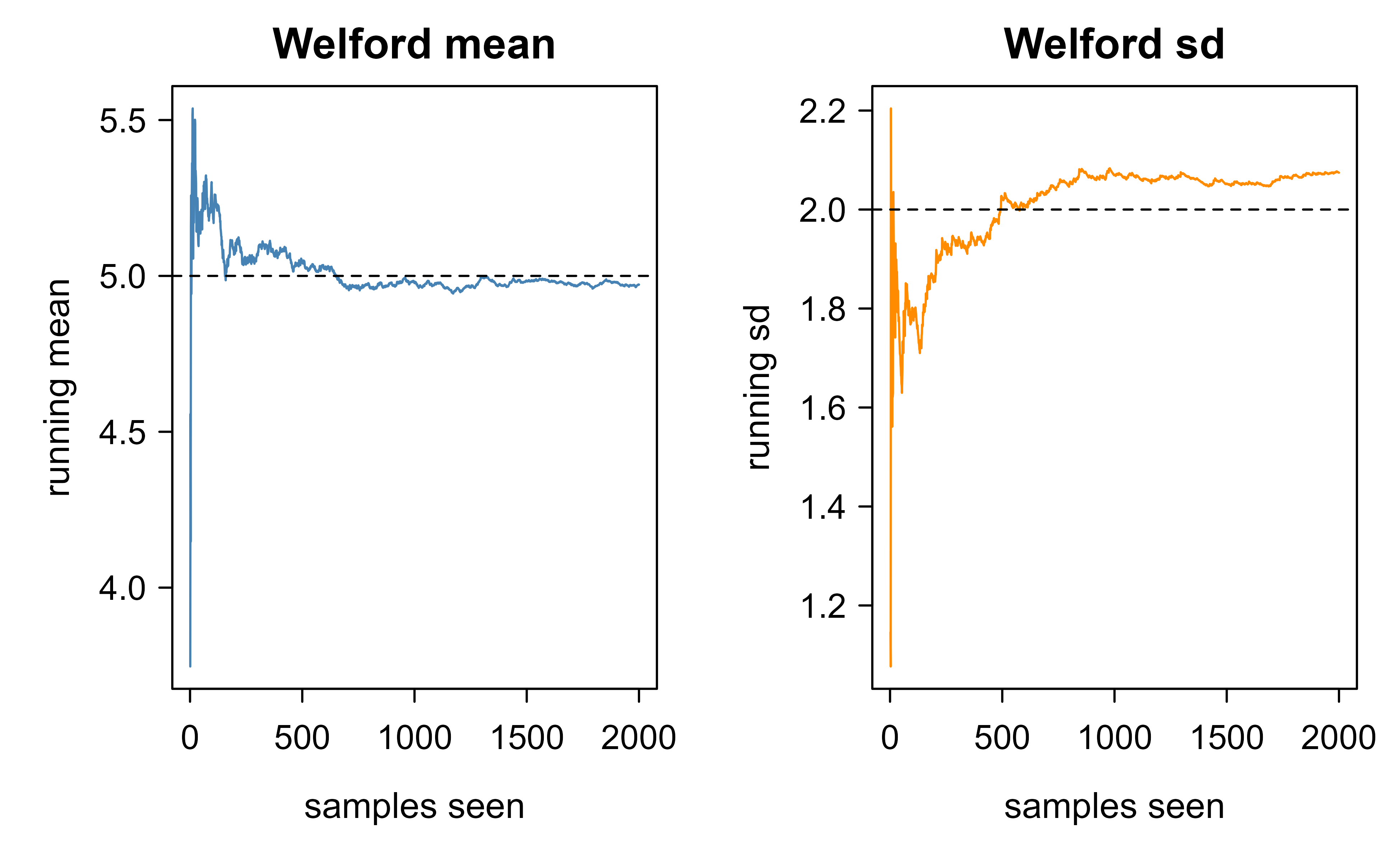
Figure 55.1 shows the running mean and standard deviation produced by the code below as the stream grows.
Show code
set.seed(1)welford_update<-function(state, x){state$n<-state$n+1Ldelta<-x-state$meanstate$mean<-state$mean+delta/state$ndelta2<-x-state$meanstate$M2<-state$M2+delta*delta2state}welford_variance<-function(state){if(state$n<2L)return(NA_real_)state$M2/(state$n-1L)}true_mu<-5true_sd<-2stream<-rnorm(2000, mean =true_mu, sd =true_sd)state<-list(n =0L, mean =0, M2 =0)running_mean<-numeric(length(stream))running_sd<-numeric(length(stream))for(iinseq_along(stream)){state<-welford_update(state, stream[i])running_mean[i]<-state$meanrunning_sd[i]<-sqrt(welford_variance(state))}# confirm the one-pass result matches base R on the full samplestopifnot(abs(state$mean-mean(stream))<1e-10)stopifnot(abs(welford_variance(state)-var(stream))<1e-8)op<-par(mfrow =c(1, 2), mar =c(4, 4, 2, 1))plot(running_mean, type ="l", col ="steelblue", xlab ="samples seen", ylab ="running mean", main ="Welford mean")abline(h =true_mu, lty =2)plot(running_sd, type ="l", col ="darkorange", xlab ="samples seen", ylab ="running sd", main ="Welford sd")abline(h =true_sd, lty =2)par(op)
Figure 55.1: Welford’s running mean and standard deviation converging to the true population values (dashed lines) as the stream grows. Estimates are noisy early and stabilize as more data arrives.
The checks pass and the two curves settle onto the dashed true values, which is the point: Welford reproduces the exact sample mean and variance while touching each value once and storing only three numbers, never the full vector at once.
55.6 Demo 2: Online Logistic Regression
Now a supervised case. The model is logistic regression with parameter \(\theta\) (including an intercept), predicting \(p_t = \sigma(\theta^\top x_t)\) where \(\sigma(z) = 1/(1+e^{-z})\). The per-example log loss and its gradient are
The OGD update is therefore the compact \(\theta \leftarrow \theta - \eta_t (p_t - y_t) x_t\). The gradient is just the prediction error \((p_t - y_t)\) scaled onto the input \(x_t\): predict too high and the weights move down along \(x_t\), predict too low and they move up.
The gradient identity is worth deriving once, since the same “(prediction minus target) times input” form appears throughout generalized linear models. With \(z = \theta^\top x_t\) and \(p_t = \sigma(z)\), the chain rule gives \(\nabla_\theta \ell_t = \frac{\partial \ell_t}{\partial p_t}\,\sigma'(z)\, x_t\). The log-loss derivative is \(\frac{\partial \ell_t}{\partial p_t} = -\frac{y_t}{p_t} + \frac{1-y_t}{1-p_t} = \frac{p_t - y_t}{p_t(1-p_t)}\), and the logistic derivative is \(\sigma'(z) = p_t(1-p_t)\). The factor \(p_t(1-p_t)\) cancels exactly, leaving \(\nabla_\theta \ell_t = (p_t - y_t)\, x_t\). This cancellation is not a coincidence: it is the canonical-link property of the Bernoulli GLM, under which the gradient of the negative log-likelihood is always (mean minus observation) times the covariate, with no variance factor left over.
Stochastic vs full-batch Newton
Batch logistic regression is fit by iteratively reweighted least squares, a Newton method using the Hessian \(\sum_t p_t(1-p_t) x_t x_t^\top\). The online update above is first-order: it discards curvature, which is why it needs the \(\eta_t\) schedule that IRLS does not. A middle ground, online Newton step (Hazan et al., 2007), maintains a running approximation to the inverse Hessian and attains the \(O(\log T)\) regret of Section 55.4.3 on exp-concave losses such as log loss, at \(O(d^2)\) per-step cost instead of \(O(d)\).
A subtlety hidden in the explicit update is stability under a large step. The plain rule \(\theta \leftarrow \theta - \eta_t (p_t - y_t) x_t\) can overshoot when \(\eta_t \lVert x_t\rVert^2\) is large. The implicit (proximal) update sidesteps this by solving \(\theta_{t+1} = \arg\min_\theta \big\{ \ell_t(\theta) + \tfrac{1}{2\eta_t}\lVert\theta - \theta_t\rVert^2 \big\}\), which evaluates the gradient at the new point rather than the old one. For many losses this is as cheap as the explicit step (the minimizer lies along \(x_t\), reducing it to a one-dimensional root find) and it is far more robust to step-size misspecification, which is why implicit SGD is the safer default when the input scale is not well controlled. We process one observation at a time, never re-reading past data, and we track the running average log loss to see learning happen. For an honest read on generalization we also compute, before each update, the loss on a held-out test set; this is the prequential idea of test-then-train.5
Warning
Never evaluate a temporal stream by shuffling it and taking a random train/test split. Doing so lets the model train on examples that came after the ones it is tested on, leaking the future and producing an optimistic, meaningless score. Prequential test-then-train respects the arrow of time.
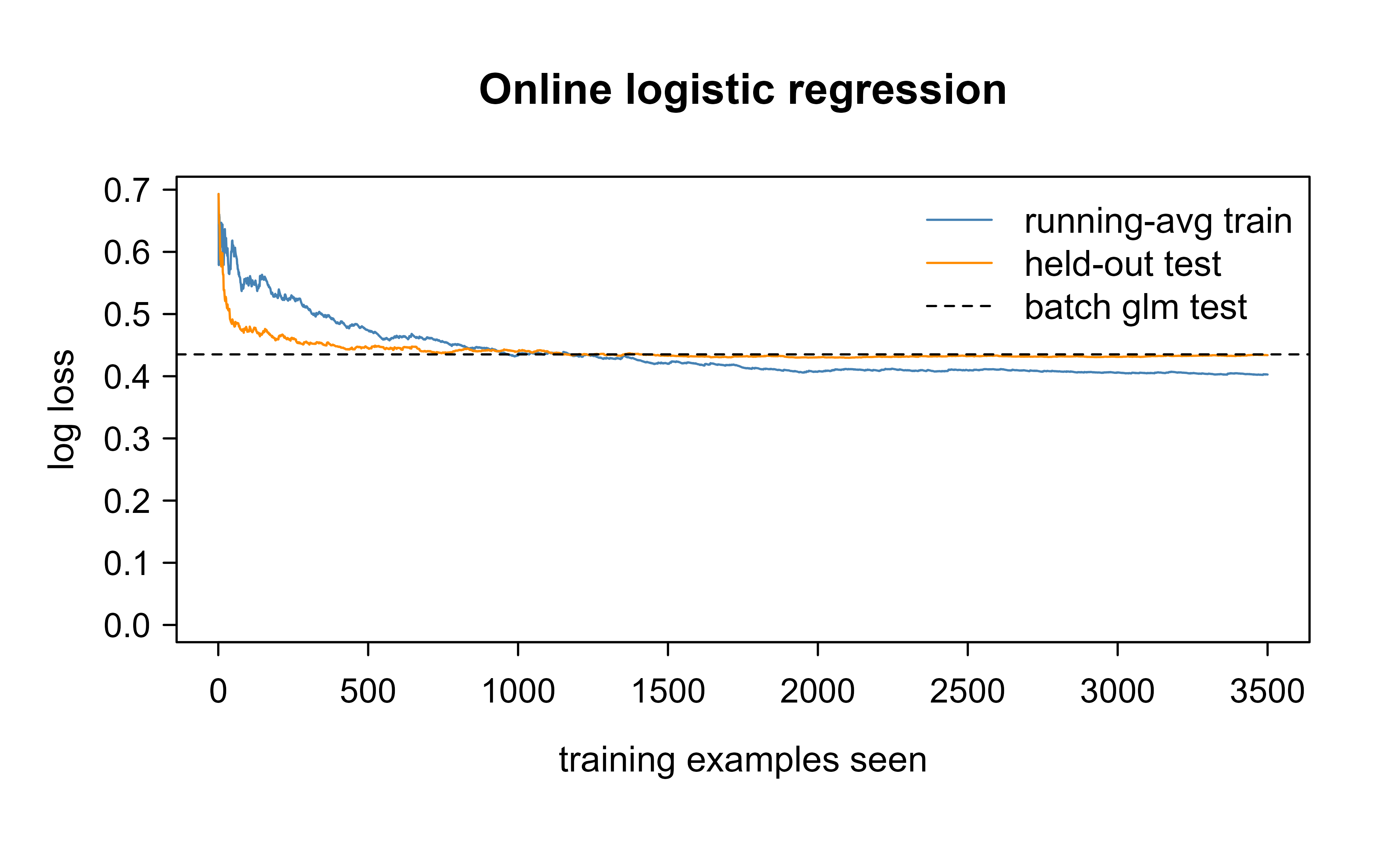
Figure 55.2 shows the resulting learning curves alongside the batch reference.
Show code
set.seed(42)sigmoid<-function(z)1/(1+exp(-z))# generate a linearly-separable-ish streamn<-4000d<-3X<-matrix(rnorm(n*d), n, d)theta_true<-c(-0.5, 1.5, -2.0, 1.0)# intercept + 3 weightsXb<-cbind(1, X)p_true<-sigmoid(Xb%*%theta_true)y<-rbinom(n, 1, p_true)# hold out a test set for prequential evaluationtest_idx<-1:500train_idx<-501:nXb_test<-Xb[test_idx, , drop =FALSE]y_test<-y[test_idx]logloss<-function(p, y){eps<-1e-12p<-pmin(pmax(p, eps), 1-eps)-mean(y*log(p)+(1-y)*log(1-p))}theta<-rep(0, d+1)# start at zeroc0<-0.5# base learning raterunning_train<-numeric(length(train_idx))test_curve<-numeric(length(train_idx))avg_loss<-0for(kinseq_along(train_idx)){i<-train_idx[k]xi<-Xb[i, ]pi<-as.numeric(sigmoid(sum(theta*xi)))# online (instantaneous) loss before updating, for the running averageinst<-logloss(pi, y[i])avg_loss<-avg_loss+(inst-avg_loss)/krunning_train[k]<-avg_loss# held-out test loss with current weights (test-then-train)p_test<-sigmoid(Xb_test%*%theta)test_curve[k]<-logloss(as.numeric(p_test), y_test)# OGD step: decaying learning rate eta_t = c0 / sqrt(t)eta<-c0/sqrt(k)theta<-theta-eta*(pi-y[i])*xi}# batch reference fit on the same training rowsbatch_fit<-glm(y~X, family =binomial, subset =train_idx)batch_test_loss<-logloss(predict(batch_fit, newdata =data.frame(X =I(X[test_idx, , drop =FALSE])), type ="response"),y_test)plot(running_train, type ="l", col ="steelblue", ylim =c(0, max(running_train)), xlab ="training examples seen", ylab ="log loss", main ="Online logistic regression")lines(test_curve, col ="darkorange")abline(h =batch_test_loss, lty =2)legend("topright", bty ="n", legend =c("running-avg train", "held-out test", "batch glm test"), col =c("steelblue", "darkorange", "black"), lty =c(1, 1, 2))round(rbind(online =theta, batch =coef(batch_fit), truth =theta_true), 3)#> (Intercept) X1 X2 X3#> online -0.466 1.441 -1.845 0.840#> batch -0.533 1.468 -1.925 0.918#> truth -0.500 1.500 -2.000 1.000
Figure 55.2: Online logistic regression trained one observation at a time. The running-average training log loss (blue) falls as the weights improve, and the held-out test log loss (orange) tracks it, confirming the streaming fit generalizes. The dashed line is the log loss of the batch glm fit on all the data.
The online weights end up close to both the batch glm estimate and the true coefficients, and the held-out loss settles near the batch model’s loss, all from a single streaming pass that stored only the current example and a parameter vector.
55.7 Trees for Streams: Hoeffding (Very Fast) Decision Trees
So far the parameters have been continuous weights that gradient descent can nudge. Trees are different: a split is a discrete choice, and the obvious way to pick the best split is to scan the whole dataset. That makes trees awkward online, because a split decision normally needs all the data at once to compare candidate features, exactly the assumption behind batch tree induction (Chapter 8). The Hoeffding tree, also called the Very Fast Decision Tree or VFDT (Domingos and Hulten, 2000), solves this with a statistical stopping rule for how much data a node needs before it can commit to a split.
The idea: at a leaf, accumulate sufficient statistics (per-feature, per-class counts) as examples stream through. Let \(G(\cdot)\) be a split-quality measure (information gain or Gini), and let \(\bar G_a\) and \(\bar G_b\) be the observed quality of the best and second-best features after \(n\) examples have reached the leaf. The Hoeffding bound says that, with probability \(1-\delta\), the true mean of a bounded quantity in range \([0,R]\) is within
of its observed average. So if \(\bar G_a - \bar G_b > \epsilon\), then with confidence \(1-\delta\) feature \(a\) really is the best split, and the node can split now without waiting for more data. As \(n\) grows, \(\epsilon\) shrinks, so even near-ties eventually resolve.
The bound is the additive Hoeffding inequality applied to the per-example split-quality differences. Let \(D_i = G_a^{(i)} - G_b^{(i)} \in [-R, R]\) be the contribution of the \(i\)-th example to the gap between the two candidate features, with sample mean \(\bar D = \bar G_a - \bar G_b\) and true mean \(\mu_D\). Hoeffding’s inequality states that for independent variables bounded in a range of width \(w\) (here \(w = 2R\) if we work with the gap directly, or \(w = R\) per-quality term), \(\Pr(\bar D - \mu_D \le -\epsilon) \le \exp(-2 n \epsilon^2 / w^2)\). Setting the right side to \(\delta\) and solving for \(\epsilon\) gives \(\epsilon = w\sqrt{\ln(1/\delta)/(2n)}\), which is the displayed formula with \(w = R\) in the convention used above. The chain of logic is then: with probability \(1-\delta\), \(\mu_D \ge \bar D - \epsilon\), so if \(\bar D > \epsilon\) we have \(\mu_D > 0\), meaning feature \(a\) has genuinely higher expected quality than feature \(b\). The error probability \(\delta\) is per split decision; over a tree with \(S\) splits a union bound gives total failure probability at most \(S\delta\), which is why \(\delta\) is set extremely small (the pseudocode uses \(10^{-7}\)).
The payoff is a consistency guarantee. Domingos and Hulten show that the expected disagreement between a Hoeffding tree and the batch tree that would be built from infinite data is bounded by \(\delta / p\), where \(p\) is the leaf probability, so the streaming tree converges to the batch tree as \(\delta \to 0\) and \(n \to \infty\). Crucially the data needed at each node to make a decision is \(O(R^2 \ln(1/\delta)/\Delta^2)\), where \(\Delta\) is the true quality gap, independent of the total stream length, so memory stays bounded even on an infinite stream.
The tie-breaking parameter
When two features are genuinely almost equal (\(\Delta \approx 0\)), \(\epsilon\) may never fall below \(\bar G_a - \bar G_b\), and the node would wait forever accumulating examples. The tie threshold \(\tau\) in the pseudocode forces a split once \(\epsilon < \tau\), on the reasoning that if the two best features are within \(\tau\) of each other it does not matter which one is chosen. Omitting \(\tau\) is a classic VFDT implementation bug that stalls tree growth on correlated features.
Intuition
The Hoeffding bound answers “have I seen enough examples to be sure the leading feature really is leading, and is not ahead by luck?” When the gap between the top two features is larger than the statistical wiggle room \(\epsilon\), the answer is yes and the node commits. The remarkable part is that this lets a single streaming pass build a tree whose splits match, with high probability, what a batch tree would have chosen on the same data, while reading each example only once.
Table 55.2 contrasts the streaming tree with its batch ancestors.
Table 55.2: Batch decision-tree induction versus the Hoeffding (Very Fast) Decision Tree, compared by number of passes, memory footprint, split criterion, data regime, and drift handling.
Aspect
Batch CART / C4.5
Hoeffding tree (VFDT)
Passes over data
Many
One
Memory
Grows with data
Bounded per node (sufficient statistics)
Split rule
Best split on full data
Split when \(\bar G_a - \bar G_b > \epsilon\)
Suited to
Finite datasets
Unbounded streams
Drift handling
Refit from scratch
Extensions (CVFDT, Hoeffding Adaptive Tree)
Production stream-mining libraries (for example MOA in Java, and river in Python) implement VFDT and its drift-aware variants. R does not ship a maintained streaming-tree package, so the snippet below is illustrative pseudocode marked eval=FALSE: it shows the split-decision logic, not a full tree implementation.
Show code
# Hoeffding split test at a leaf (illustrative).# counts: accumulated sufficient statistics at this leaf.hoeffding_epsilon<-function(R, n, delta){sqrt((R^2*log(1/delta))/(2*n))}should_split<-function(gain_best, gain_second, n,R=1, delta=1e-7, tau=0.05){eps<-hoeffding_epsilon(R, n, delta)diff<-gain_best-gain_second# split if the best feature clearly wins, OR if the contest is# effectively tied (diff < eps < tau) so waiting is pointless(diff>eps)||(eps<tau)}
55.8 Concept Drift
Everything so far assumed that the world a model learns is the world it is later tested on. Streams break that assumption: over time the joint distribution \(P_t(x, y)\) drifts. Diagnosing the kind of drift matters because the fix differs, so it helps to keep three cases straight.
Covariate shift (virtual drift): \(P(x)\) changes but \(P(y \mid x)\) does not. The decision boundary still holds, but inputs move into regions the model saw little of.
Real concept drift: \(P(y \mid x)\) changes, so the optimal boundary itself moves. This is what degrades a fixed model’s accuracy.
Drift can also differ in speed: abrupt (a sudden regime change), gradual (one concept fades as another grows), or recurring (seasonal patterns that return).
Note
The distinction between covariate shift and real drift is practical, not academic. Covariate shift often just means the model needs more coverage of the newly common inputs; real drift means the model’s current answer is now wrong and it has to forget. Misdiagnosing one as the other wastes effort.
No single mechanism handles every kind of drift, so production systems combine several. The main families are these.
Forgetting through the learning rate. A non-decaying or slowly-decaying \(\eta_t\) keeps the model plastic so recent examples dominate. The cost is more variance and never fully converging.
Sliding windows. Train on the last \(w\) examples and drop older ones. Window size sets the bias-variance and stability-plasticity trade-off: short windows adapt fast but are noisy.
Explicit drift detectors. ADWIN (Adaptive Windowing, Bifet and Gavalda, 2007) maintains a variable-length window and shrinks it when a statistically significant change in the mean error is detected; DDM (Drift Detection Method, Gama et al., 2004) watches the online error rate and signals warning and drift thresholds. On a signal, the model is reset or retrained on recent data.
The two detectors rest on different statistical tests, and knowing which is worth a paragraph each. ADWIN keeps a window \(W\) of recent error indicators and, conceptually, checks every split of \(W\) into an older sub-window \(W_0\) (size \(n_0\), mean \(\hat\mu_0\)) and a newer one \(W_1\) (size \(n_1\), mean \(\hat\mu_1\)). It declares drift when \(|\hat\mu_0 - \hat\mu_1| > \epsilon_{\text{cut}}\), where the cut threshold comes from a Hoeffding-style bound on the difference of two means,
with \(m\) the harmonic mean of the sub-window sizes. When the test fires, the older portion is dropped, so the window length itself becomes an estimate of how far back the current concept extends. ADWIN comes with a rigorous false-positive rate bounded by \(\delta\) and a false-negative bound that shrinks with the magnitude of the change, and an efficient exponential-histogram implementation makes the all-splits check \(O(\log |W|)\) rather than \(O(|W|)\).
DDM takes a parametric view. If the model’s error rate is \(p_t\), the number of errors in \(t\) trials is binomial, so the standard deviation of the running error rate is \(s_t = \sqrt{p_t(1-p_t)/t}\). DDM tracks the minimum of \(p_t + s_t\) seen so far, call it \((p_{\min}, s_{\min})\), on the premise that a stationary learner’s error should only decrease. It raises a warning when \(p_t + s_t \ge p_{\min} + 2 s_{\min}\) and declares drift at \(p_t + s_t \ge p_{\min} + 3 s_{\min}\), the familiar two-sigma and three-sigma control-chart limits. Examples seen since the warning are buffered to train the replacement model, so that when drift is confirmed a fresh model is already warmed up. DDM detects abrupt drift well but is slow on gradual drift, which is exactly the regime where ADWIN’s nonparametric windowing wins. - Ensembles. Keep a pool of models trained on different recent segments and weight them by recent accuracy, retiring stale members; this is ensemble learning (Chapter 57) adapted to a moving distribution.
A concrete decision rule: if accuracy is drifting, first check whether \(P(x)\) moved (cheap to monitor) before assuming \(P(y\mid x)\) did. Covariate shift often just needs more coverage or reweighting, while real drift needs the model to forget.
55.9 Practical Guidance and Pitfalls
With the machinery in hand, the final question is when to actually use it. Online learning is the right call when any of the following holds.
The data is too large for memory or never ends.
Predictions and updates must happen in real time with bounded per-step cost.
The target distribution moves and you cannot retrain fast enough to keep up.
Prefer batch learning in the opposite situation.
The dataset is finite and fits in memory, and the distribution is stable. Batch optimization is more sample-efficient per example and easier to validate; online learning buys you nothing here and adds operational complexity.
Even when online learning is warranted, a handful of mistakes account for most failures in practice. The list below collects the ones worth memorizing.
Learning rate. Too large diverges or oscillates; too small crawls and never catches drift. Start with a decaying schedule such as \(\eta_t = c/\sqrt{t}\) and tune \(c\) on a replayed stream. If you need permanent adaptation, cap the decay so \(\eta_t\) never falls below a floor.
Feature scaling on the fly. Standardize with running statistics (Welford), not a fixed scaler computed from an early batch, or the scale will be wrong once the stream drifts.
Evaluation. Do not shuffle a temporal stream and do a random split; that leaks the future. Use prequential evaluation (test-then-train) so each example is scored before it is learned from.
Single example variance. Per-example gradients are noisy. Small mini-batches (10 to 100) smooth the updates while keeping the streaming property.
Catastrophic forgetting and label delay. If labels arrive late (a click is known only later), align the update to when the label actually lands, not when the features arrived.
Stateful bugs. Online systems carry state across time, so a bad update can corrupt the model permanently. Keep a periodic checkpoint and a guardrail metric that can trigger a rollback.
Tip
The single highest-leverage safeguard for a production online learner is a checkpoint plus a rollback trigger. Because the model’s state evolves continuously, one pathological batch of inputs can poison it for good; being able to revert to last night’s snapshot turns a permanent outage into a brief blip.
To summarize the chapter in one breath: online learning replaces “fit once, ship, retrain later” with “update on every example, forever.” The same gradient step (\(\theta_{t+1} = \theta_t - \eta_t g_t\)) drives the perceptron, online logistic regression, and general OGD; stochastic approximation explains when it converges and regret measures it when it cannot; Hoeffding trees bring the streaming discipline to discrete split decisions; and concept drift, together with leak-free prequential evaluation and a sane learning rate, is where the real engineering lives.
55.10 Further Reading
Rosenblatt, F. (1958). The perceptron: a probabilistic model for information storage and organization in the brain. Psychological Review. Original perceptron.
Robbins, H., and Monro, S. (1951). A stochastic approximation method. Annals of Mathematical Statistics. Foundation of stochastic approximation.
Welford, B. P. (1962). Note on a method for calculating corrected sums of squares and products. Technometrics. The streaming variance update.
Zinkevich, M. (2003). Online convex programming and generalized infinitesimal gradient ascent. ICML. Online gradient descent and \(O(\sqrt{T})\) regret.
Hazan, E., Agarwal, A., and Kale, S. (2007). Logarithmic regret algorithms for online convex optimization. Machine Learning. The \(O(\log T)\) rate for strongly convex and exp-concave losses, and the online Newton step.
Duchi, J., Hazan, E., and Singer, Y. (2011). Adaptive subgradient methods for online learning and stochastic optimization. JMLR. AdaGrad.
McMahan, H. B., et al. (2013). Ad click prediction: a view from the trenches. KDD. FTRL-Proximal for sparse online learning at scale.
Cesa-Bianchi, N., and Lugosi, G. (2006). Prediction, Learning, and Games. Cambridge University Press. Comprehensive treatment of regret and online learning.
Shalev-Shwartz, S. (2012). Online learning and online convex optimization. Foundations and Trends in Machine Learning. Modern survey with proofs.
Domingos, P., and Hulten, G. (2000). Mining high-speed data streams. KDD. The Hoeffding tree / VFDT.
Gama, J., Medas, P., Castillo, G., and Rodrigues, P. (2004). Learning with drift detection. SBIA. The DDM drift detector.
Bifet, A., and Gavalda, R. (2007). Learning from time-changing data with adaptive windowing. SDM. The ADWIN algorithm.
Bifet, A., Gavalda, R., Holmes, G., and Pfahringer, B. (2018). Machine Learning for Data Streams. MIT Press. Book-length treatment, with the MOA framework.
Bottou, L., Curtis, F. E., and Nocedal, J. (2018). Optimization methods for large-scale machine learning. SIAM Review. Stochastic gradient methods at scale.
This \(O(1)\) per-step cost is the property that makes a stream of unbounded length feasible at all: whether you have seen a thousand examples or a billion, the work to absorb the next one is the same.↩︎
The learning rate controls how far each example is allowed to move the parameters. It is the single most important knob in online learning, and most of the failure modes in Section 55.9 trace back to choosing it badly.↩︎
A (sub)gradient generalizes the gradient to functions with kinks. The perceptron loss has a corner at \(y_t\theta^\top x_t = 0\); one valid subgradient there is \(0\), which is why a correct prediction triggers no update.↩︎
A root of \(h\) is a value of \(\theta\) where \(h(\theta)=0\). When \(h\) is the gradient of a smooth convex risk, its root is the risk minimizer, so root-finding and minimization coincide.↩︎
Prequential (predictive-sequential) evaluation scores each example with the current model before that example is used to update it. Because the model never sees an example’s label until after it has been graded on it, no future information leaks into the score, so prequential loss is an unbiased running estimate of how the deployed model is doing.↩︎
Source Code
# Online and Streaming Learning {#sec-online-learning}```{r}#| include: falsesource("_common.R")```Most of this book assumes a fixed training set: you collect $n$ observations, fit a model, and evaluate it. Online learning drops that assumption. Data arrive one observation (or one small batch) at a time, the model updates immediately, and the old data may never be stored again. This is the natural setting for systems that must keep learning in production: fraud scoring, recommendation, ad ranking, sensor monitoring, and any service where the data distribution moves over time.This chapter develops the core ideas: the incremental update view of learning, the perceptron and online gradient descent, the stochastic approximation theory that explains why these updates converge, regret as the right notion of performance, Hoeffding (very fast) decision trees for unbounded streams, and concept drift. The runnable demos are implemented in base R so the mechanics are fully visible: a streaming mean and variance with Welford's algorithm, and an online logistic regression that updates one observation at a time.::: {.callout-tip title="Intuition"}Batch learning is like studying for an exam from a fixed textbook. Online learning is like a person who has to answer questions all day long, learning a little from each one as soon as they find out whether they were right, and never getting to reread the earlier questions. The skill is to improve continuously from a single forward pass through experience.:::By the end you should be able to recognize when a problem calls for streaming methods rather than periodic retraining, write a simple incremental update by hand, reason about whether it will converge, and avoid the operational traps (leaky evaluation, runaway learning rates, silent drift) that make online systems fail in production.## Where Online Learning FitsIn a batch workflow you retrain on a schedule (nightly, weekly) and ship a new model. That works well for many problems, but it breaks down in two situations:- The data does not fit in memory, or the stream never ends, so there is no "full" training set to hold.- The relationship between features and target changes faster than your retraining cadence, so a model trained last week is already stale.Online learning addresses both. Each example is processed once, used to update the model, and discarded. Memory and per-step compute stay constant regardless of how many examples have been seen.^[This $O(1)$ per-step cost is the property that makes a stream of unbounded length feasible at all: whether you have seen a thousand examples or a billion, the work to absorb the next one is the same.] Because the update is incremental, the model tracks a moving target instead of freezing at a snapshot.To place online learning next to its relatives, @tbl-online-learning-paradigm-comparison contrasts how each style accesses data, what it costs, and where it shines.| Property | Batch learning | Mini-batch SGD | Online / streaming ||---|---|---|---|| Data access | Full set, many passes | Full set, shuffled batches | One pass, one example at a time || Memory | $O(n)$ | $O(\text{batch})$ | $O(1)$ in the number of examples || Update timing | After full fit | After each batch | After each example || Adapts to drift | Only on retrain | Only on retrain | Continuously || Typical use | Stable tabular problems | Deep nets, large but finite data | Production streams, huge or infinite data |: Comparison of batch, mini-batch, and online learning paradigms by data access pattern, memory cost, update timing, and suitability for drifting distributions. {#tbl-online-learning-paradigm-comparison}A common production pattern is a hybrid: train a strong batch model offline, then keep a lightweight online layer (a logistic regression or a small set of weights) updating on the live stream to absorb short-term drift, retraining the heavy model on a slower clock.::: {.callout-tip title="When to use this"}Reach for a streaming method when the data is too big to store, never stops arriving, or moves faster than you can retrain. If your dataset is finite, fits in memory, and comes from a stable distribution, batch learning is simpler to validate and usually more accurate per example. @sec-practical-guidance-and-pitfalls returns to this decision in detail.:::## The Incremental Update View {#sec-the-incremental-update-view}Write the model as a parameter vector $\theta \in \mathbb{R}^d$. At step $t$ the learner holds $\theta_t$, sees an example $(x_t, y_t)$, suffers a loss $\ell_t(\theta_t) = \ell(\theta_t; x_t, y_t)$, and produces $\theta_{t+1}$. The generic online update is$$\theta_{t+1} = \theta_t - \eta_t \, g_t, \qquad g_t = \nabla_\theta \ell_t(\theta_t),$$where $\eta_t > 0$ is a step size (learning rate)^[The learning rate controls how far each example is allowed to move the parameters. It is the single most important knob in online learning, and most of the failure modes in @sec-practical-guidance-and-pitfalls trace back to choosing it badly.] and $g_t$ is the gradient of the current example's loss. Two features make this practical: the update touches only the current example, and the cost per step does not grow with $t$.::: {.callout-important title="Key idea"}Almost every online method in this chapter is a special case of $\theta_{t+1} = \theta_t - \eta_t g_t$. Change the loss $\ell_t$ and you change the algorithm; the update template stays the same. Recognizing this one line under different disguises is most of what it takes to read the online-learning literature.:::Even a running average is an instance of this template. If $\ell_t(\theta) = \tfrac12 (\theta - x_t)^2$ then $g_t = \theta_t - x_t$, and with $\eta_t = 1/t$ the update$$\theta_{t+1} = \theta_t - \tfrac{1}{t}(\theta_t - x_t)$$reproduces the exact sample mean of $x_1, \dots, x_t$. This is the bridge to stochastic approximation below.To see that the $\eta_t = 1/t$ update is not merely an analogy but an exact algebraic identity, expand it. Write $\bar x_t = \theta_{t+1}$ for the estimate after $t$ points. Then$$\theta_{t+1} = \theta_t - \tfrac{1}{t}(\theta_t - x_t) = \Big(1 - \tfrac{1}{t}\Big)\theta_t + \tfrac{1}{t} x_t = \tfrac{t-1}{t}\theta_t + \tfrac{1}{t} x_t .$$Multiplying through by $t$ gives $t\,\theta_{t+1} = (t-1)\theta_t + x_t$. If $\theta_t = \tfrac1{t-1}\sum_{i=1}^{t-1} x_i$ is the mean of the first $t-1$ points (the induction hypothesis), then $(t-1)\theta_t = \sum_{i=1}^{t-1} x_i$ and so $t\,\theta_{t+1} = \sum_{i=1}^{t} x_i$, i.e. $\theta_{t+1} = \tfrac1t \sum_{i=1}^t x_i$. The base case $t=1$ gives $\theta_2 = x_1$. By induction the recursion holds the exact running mean at every step, with $O(1)$ memory and no stored history. The same telescoping shows why $\eta_t = 1/t$ is the unique decaying schedule that gives each observation equal weight $1/t$ in the final average: any other schedule weights examples unequally, which is exactly what we want when the target moves (older examples should count less), and exactly what we do not want when it is stationary.## The PerceptronThe perceptron (Rosenblatt, 1958) is the earliest online classifier and the ancestor of modern neural networks (@sec-neural-networks); it is still the cleanest illustration of mistake-driven learning. Labels are $y_t \in \{-1, +1\}$ and the prediction is $\hat y_t = \operatorname{sign}(\theta_t^\top x_t)$. The update fires only on a mistake:$$\theta_{t+1} =\begin{cases}\theta_t + y_t x_t & \text{if } y_t (\theta_t^\top x_t) \le 0 \\\theta_t & \text{otherwise.}\end{cases}$$In words: if the prediction is correct, leave the weights alone; if it is wrong, nudge them toward getting that example right by adding $y_t x_t$. This is online (sub)gradient descent with step size 1 on the loss $\ell_t(\theta) = \max(0, -y_t \theta^\top x_t)$, the perceptron loss.^[A (sub)gradient generalizes the gradient to functions with kinks. The perceptron loss has a corner at $y_t\theta^\top x_t = 0$; one valid subgradient there is $0$, which is why a correct prediction triggers no update.] The classic guarantee bounds the number of mistakes rather than a probability of error, which is what makes it an online rather than a statistical result.::: {.callout-note}The mistake bound below is one of the oldest results in machine learning, and it is striking precisely because it makes no probabilistic assumption. It does not say "errors are unlikely"; it says the perceptron can make at most a fixed number of mistakes, ever, as long as the data is separable with a margin.:::Perceptron mistake bound. Suppose there is a unit vector $u$ ($\lVert u \rVert = 1$) and a margin $\gamma > 0$ with $y_t (u^\top x_t) \ge \gamma$ for all $t$, and suppose $\lVert x_t \rVert \le R$ for all $t$. Then the total number of mistakes the perceptron makes is at most$$M \le \frac{R^2}{\gamma^2}.$$Sketch. Let the updates happen on the mistake rounds. On each mistake, the projection onto $u$ grows by at least $\gamma$, because $u^\top \theta_{t+1} = u^\top \theta_t + y_t (u^\top x_t) \ge u^\top \theta_t + \gamma$, so after $M$ mistakes $u^\top \theta \ge M\gamma$. At the same time the squared norm grows slowly: on a mistake $\lVert \theta_{t+1}\rVert^2 = \lVert\theta_t\rVert^2 + 2 y_t(\theta_t^\top x_t) + \lVert x_t\rVert^2 \le \lVert\theta_t\rVert^2 + R^2$, since the mistake condition makes the middle term nonpositive, so $\lVert\theta\rVert^2 \le M R^2$. Combining with $u^\top\theta \le \lVert\theta\rVert$ gives $M\gamma \le \sqrt{M} R$, hence $M \le R^2/\gamma^2$. The bound does not depend on the dimension $d$ or the number of examples, only on the geometry (margin and radius).## Online Gradient Descent and Stochastic ApproximationOnline gradient descent (OGD) is the perceptron's general form: apply $\theta_{t+1} = \theta_t - \eta_t g_t$ for any (sub)differentiable loss. Two questions follow. Does it converge to a good parameter, and how should $\eta_t$ behave?Stochastic approximation answers the first. The Robbins-Monro method (Robbins and Monro, 1951) finds a root^[A root of $h$ is a value of $\theta$ where $h(\theta)=0$. When $h$ is the gradient of a smooth convex risk, its root is the risk minimizer, so root-finding and minimization coincide.] of $h(\theta) = \mathbb{E}[g(\theta; Z)] = 0$ using only noisy samples $g(\theta; z_t)$, with the update $\theta_{t+1} = \theta_t - \eta_t \, g(\theta_t; z_t)$. When $\theta$ minimizes a convex risk $R(\theta) = \mathbb{E}[\ell(\theta; Z)]$, the root of the gradient is exactly the minimizer, so OGD on a stream of i.i.d. examples is Robbins-Monro applied to $h = \nabla R$. Convergence holds under the step-size conditions$$\sum_{t=1}^\infty \eta_t = \infty, \qquad \sum_{t=1}^\infty \eta_t^2 < \infty.$$These two conditions encode a tug-of-war. The first condition keeps the steps large enough in aggregate to reach the solution from any start; the second forces the steps to shrink fast enough that gradient noise averages out. The canonical choice $\eta_t = c/t$ satisfies both. In practice $\eta_t = c/\sqrt{t}$ (which violates the second condition) is common because it adapts better when the target moves, trading exact convergence for responsiveness.::: {.callout-tip title="Intuition"}A step size that decays too slowly leaves the model permanently jittery, chasing noise. One that decays too fast freezes the model before it has reached a good answer. The $\sum\eta_t=\infty,\ \sum\eta_t^2<\infty$ pair is the precise statement of "fast enough to settle, slow enough to arrive.":::### Regret: the right scorecardWhen data is not i.i.d. (it may be adversarial, or drifting), "convergence to the risk minimizer" is not well defined, so online learning is judged by regret. After $T$ rounds, regret compares the learner's cumulative loss to the best single fixed parameter chosen in hindsight:$$\text{Regret}_T = \sum_{t=1}^T \ell_t(\theta_t) - \min_{\theta \in \Theta} \sum_{t=1}^T \ell_t(\theta).$$An algorithm is "no-regret" if $\text{Regret}_T / T \to 0$, meaning its average loss approaches that of the best fixed parameter, whatever the sequence. For convex losses with bounded gradients ($\lVert g_t \rVert \le G$) and a bounded domain ($\lVert \theta \rVert \le D$), OGD with $\eta_t = D/(G\sqrt{t})$ achieves (Zinkevich, 2003)$$\text{Regret}_T \le \tfrac{3}{2} G D \sqrt{T} = O(\sqrt{T}).$$Sublinear $O(\sqrt{T})$ regret means the per-round penalty for not knowing the future vanishes as $\sqrt{T}/T = 1/\sqrt{T}$. This is the central performance promise of online convex optimization and it requires no statistical assumption on how the data is generated.::: {.callout-important title="Key idea"}Regret reframes the goal. Instead of asking "did we recover the true model?" (which assumes there is one), it asks "did we do nearly as well as the best fixed model we could have picked with hindsight?" That question stays meaningful even when an adversary chooses the data, which is why regret, not risk, is the native scorecard of online learning.:::### Deriving the $O(\sqrt{T})$ regret bound {#sec-online-learning-ogd-regret-proof}The $O(\sqrt T)$ bound is not folklore; it follows from one short potential argument that is worth seeing in full, because it also reveals exactly which assumptions are load-bearing. Assume each $\ell_t$ is convex with subgradient $g_t \in \partial \ell_t(\theta_t)$ satisfying $\lVert g_t\rVert \le G$, and that the feasible set $\Theta$ is convex with diameter $\lVert \theta - \theta'\rVert \le D$ for $\theta, \theta' \in \Theta$. Projected OGD is $\theta_{t+1} = \Pi_\Theta(\theta_t - \eta_t g_t)$, where $\Pi_\Theta$ is Euclidean projection onto $\Theta$.Fix any comparator $\theta^\star \in \Theta$. The potential is the squared distance $\lVert \theta_t - \theta^\star\rVert^2$. Projection onto a convex set is nonexpansive, $\lVert \Pi_\Theta(v) - \theta^\star\rVert \le \lVert v - \theta^\star\rVert$ for $\theta^\star\in\Theta$, so$$\lVert \theta_{t+1} - \theta^\star\rVert^2 \le \lVert \theta_t - \eta_t g_t - \theta^\star\rVert^2= \lVert \theta_t - \theta^\star\rVert^2 - 2\eta_t\, g_t^\top(\theta_t - \theta^\star) + \eta_t^2 \lVert g_t\rVert^2 .$$Rearranging for the inner product and using convexity ($\ell_t(\theta_t) - \ell_t(\theta^\star) \le g_t^\top(\theta_t - \theta^\star)$),$$\ell_t(\theta_t) - \ell_t(\theta^\star) \;\le\; \frac{\lVert \theta_t - \theta^\star\rVert^2 - \lVert \theta_{t+1} - \theta^\star\rVert^2}{2\eta_t} + \frac{\eta_t}{2}\lVert g_t\rVert^2 .$$Sum over $t = 1, \dots, T$. With a constant step $\eta_t = \eta$ the first term telescopes to $\big(\lVert\theta_1-\theta^\star\rVert^2 - \lVert\theta_{T+1}-\theta^\star\rVert^2\big)/(2\eta) \le D^2/(2\eta)$, and the second is bounded by $\eta T G^2/2$, giving$$\text{Regret}_T \le \frac{D^2}{2\eta} + \frac{\eta T G^2}{2}.$$ {#eq-online-learning-ogd-regret}Minimizing the right side over $\eta$ sets $\eta^\star = D/(G\sqrt T)$, which yields $\text{Regret}_T \le DG\sqrt T$. With the time-varying schedule $\eta_t = D/(G\sqrt t)$ (which needs no advance knowledge of $T$) the same summation, using $\sum_{t=1}^T 1/\sqrt t \le 2\sqrt T$, gives the stated $\text{Regret}_T \le \tfrac32 GD\sqrt T$. The proof exposes the trade-off behind the step-size conditions of @sec-the-incremental-update-view in static form: shrinking $\eta$ kills the noise term $\eta_t \lVert g_t\rVert^2/2$ but inflates the distance term $D^2/(2\eta)$, and $\eta \propto 1/\sqrt t$ balances the two.The simulation below confirms the $O(\sqrt T)$ scaling empirically on a stream of random linear losses inside the unit ball: it runs projected OGD, records the realized regret against the best fixed point in hindsight, and checks that regret divided by $\sqrt T$ stays bounded (does not grow) as $T$ increases.```{r ogd-regret-check, message=FALSE, warning=FALSE}set.seed(7)d <-5D <-1# domain radius (unit ball)proj_ball <-function(v, r = D) { # project onto radius-r ball nrm <-sqrt(sum(v^2))if (nrm > r) v * (r / nrm) else v}run_ogd <-function(Tn) { G <-1# gradient bound grads <-matrix(runif(Tn * d, -1, 1), Tn, d) grads <- grads /sqrt(rowSums(grads^2)) # unit-norm gradients, ||g||=1 theta <-rep(0, d) cum_learner <-0 G_sum <-rep(0, d) # for the comparator thetas <-matrix(0, Tn, d)for (t in1:Tn) { eta <- D / (G *sqrt(t)) cum_learner <- cum_learner +sum(grads[t, ] * theta) # linear loss g_t' theta G_sum <- G_sum + grads[t, ] theta <-proj_ball(theta - eta * grads[t, ]) }# best fixed point in hindsight minimizes sum_t g_t' theta over the ball:# theta* = -D * G_sum / ||G_sum|| best <--D * G_sum /sqrt(sum(G_sum^2)) cum_best <-sum(G_sum * best) cum_learner - cum_best}Ts <-c(250, 1000, 4000, 16000)reg <-sapply(Ts, run_ogd)data.frame(T = Ts, regret =round(reg, 2),regret_over_sqrtT =round(reg /sqrt(Ts), 3))```The last column stays roughly flat as $T$ grows by orders of magnitude, confirming $\text{Regret}_T = O(\sqrt T)$: the normalized quantity neither blows up nor heads to zero, exactly as the balanced bound @eq-online-learning-ogd-regret predicts once $\eta$ is tuned to $1/\sqrt T$.### Strong convexity gives $O(\log T)$ {#sec-online-learning-strong-convex}If each loss is not just convex but $\mu$-strongly convex, meaning $\ell_t(\theta^\star) \ge \ell_t(\theta_t) + g_t^\top(\theta^\star - \theta_t) + \tfrac{\mu}{2}\lVert\theta^\star - \theta_t\rVert^2$, the regret drops from $\sqrt T$ to $\log T$. Carrying the extra quadratic term through the same expansion gives$$\ell_t(\theta_t) - \ell_t(\theta^\star) \le \frac{\lVert \theta_t - \theta^\star\rVert^2 - \lVert \theta_{t+1} - \theta^\star\rVert^2}{2\eta_t} - \frac{\mu}{2}\lVert\theta_t - \theta^\star\rVert^2 + \frac{\eta_t}{2}\lVert g_t\rVert^2 .$$Choose the schedule $\eta_t = 1/(\mu t)$ and write $a_t = \lVert\theta_t - \theta^\star\rVert^2$. The distance contribution at round $t$ is $\tfrac{1}{2\eta_t}(a_t - a_{t+1}) - \tfrac{\mu}{2}a_t = \tfrac{\mu t}{2}(a_t - a_{t+1}) - \tfrac{\mu}{2}a_t = \tfrac{\mu}{2}\big[(t-1)a_t - t\,a_{t+1}\big]$. Summed over $t = 1, \dots, T$ this telescopes to $\tfrac{\mu}{2}\big[0 \cdot a_1 - T a_{T+1}\big] \le 0$. Only the gradient-noise term survives, and with $\eta_t = 1/(\mu t)$ it is $\sum_t \tfrac{\eta_t}{2}\lVert g_t\rVert^2 \le \tfrac{G^2}{2\mu}\sum_t \tfrac1t$, so$$\text{Regret}_T \le \frac{G^2}{2\mu}\sum_{t=1}^T \frac1t \le \frac{G^2}{2\mu}\big(1 + \ln T\big) = O(\log T).$$This is the online analogue of the familiar fact that strongly convex risks are learned at the fast $1/t$ rate rather than the slow $1/\sqrt t$ rate, and it is why an $\ell_2$ penalty (which makes any convex loss $\mu$-strongly convex) both regularizes and accelerates an online learner. Regularized OGD on $\ell_t(\theta) + \tfrac{\lambda}{2}\lVert\theta\rVert^2$ uses the schedule $\eta_t = 1/(\lambda t)$ and enjoys the logarithmic bound automatically.::: {.callout-note}The two rates, $\sqrt T$ for convex and $\log T$ for strongly convex, are both optimal: no online algorithm can beat $\Omega(\sqrt T)$ on general convex losses or $\Omega(\log T)$ on strongly convex ones (Abernethy et al., 2008; Hazan et al., 2007). OGD is therefore minimax optimal up to constants in both regimes, which is part of why such a simple update is so durable.:::### Adaptive step sizes: AdaGrad and FTRL {#sec-online-learning-adagrad}A fixed $\eta_t \propto 1/\sqrt t$ treats every coordinate the same, which is wasteful when features differ wildly in scale or frequency (common with sparse, high-dimensional streams such as text or click data). AdaGrad (Duchi, Hazan, and Singer, 2011) gives each coordinate its own learning rate that shrinks in proportion to the accumulated gradient energy on that coordinate. Let $G_{t,j} = \sum_{s=1}^t g_{s,j}^2$ be the running sum of squared gradients for coordinate $j$. The update is$$\theta_{t+1,j} = \theta_{t,j} - \frac{\eta}{\sqrt{G_{t,j} + \epsilon}}\, g_{t,j} ,$$with $\epsilon > 0$ for numerical safety. Coordinates that receive large or frequent gradients get small steps; rare but informative coordinates keep large steps. AdaGrad attains regret $O\big(D_\infty \sum_j \lVert g_{1:T,j}\rVert_2\big)$ (equivalently $O\big(\sum_j \sqrt{\sum_{t=1}^T g_{t,j}^2}\big)$ up to the domain factor), which is $O(d\sqrt T)$ in the worst case but can be much smaller than the dimension-blind $GD\sqrt T$ when gradients are sparse. Its one weakness is that $G_{t,j}$ grows monotonically, so the effective rate decays to zero, which is fatal under drift; RMSProp and Adam replace the sum with an exponential moving average $G_{t,j} = \beta G_{t-1,j} + (1-\beta) g_{t,j}^2$ precisely to keep the learner plastic.These updates are special cases of Follow-The-Regularized-Leader (FTRL), the unifying view of online convex optimization. FTRL plays, at each round, the minimizer of all past losses plus a regularizer,$$\theta_{t+1} = \arg\min_{\theta \in \Theta} \Big\{ \sum_{s=1}^t g_s^\top \theta + \psi_t(\theta) \Big\} .$$With $\psi_t(\theta) = \tfrac{1}{2\eta}\lVert\theta\rVert^2$ this linearized FTRL reduces exactly to OGD; with a per-coordinate quadratic $\psi_t(\theta) = \tfrac12\sum_j \sqrt{G_{t,j}}\,\theta_j^2$ it reduces to AdaGrad. FTRL-Proximal with an $\ell_1$ term is the workhorse behind production click-through-rate models (McMahan et al., 2013) because it yields exactly sparse weight vectors online, something plain OGD with subgradients of $\lVert\theta\rVert_1$ does not achieve.## Demo 1: Streaming Mean and Variance (Welford)We start with the simplest possible streaming statistic, a running mean and variance, because it shows the incremental update template at its barest and introduces a numerical pitfall worth knowing.A naive streaming variance that accumulates $\sum x$ and $\sum x^2$ and then computes $\frac{1}{n-1}(\sum x^2 - n\bar x^2)$ can lose precision badly: when the two large sums are close, subtracting them cancels most of the significant digits, and the result can even come out negative. Welford's algorithm (Welford, 1962) avoids this by updating the mean and the sum of squared deviations $M_2 = \sum_i (x_i - \bar x)^2$ in one pass with good numerical behavior. With $\bar x_t$ the mean after $t$ points,$$\bar x_t = \bar x_{t-1} + \frac{x_t - \bar x_{t-1}}{t}, \qquadM_{2,t} = M_{2,t-1} + (x_t - \bar x_{t-1})(x_t - \bar x_t),$$and the sample variance is $s_t^2 = M_{2,t} / (t-1)$. Each step is $O(1)$ in time and memory. Notice that the mean update $\bar x_t = \bar x_{t-1} + (x_t - \bar x_{t-1})/t$ is exactly the running-average special case from @sec-the-incremental-update-view, with the gradient $g_t = \theta_t - x_t$ and step size $\eta_t = 1/t$.The $M_2$ update is not an approximation; it is an exact identity, and deriving it shows where the curious cross term $(x_t - \bar x_{t-1})(x_t - \bar x_t)$ comes from. By definition $M_{2,t} = \sum_{i=1}^t (x_i - \bar x_t)^2$. Split off the newest point and rewrite the older deviations around the new mean:$$M_{2,t} - M_{2,t-1} = (x_t - \bar x_t)^2 + \sum_{i=1}^{t-1}\big[(x_i - \bar x_t)^2 - (x_i - \bar x_{t-1})^2\big] .$$Factor each bracket as a difference of squares, $(x_i - \bar x_t)^2 - (x_i - \bar x_{t-1})^2 = (\bar x_{t-1} - \bar x_t)\big(2 x_i - \bar x_t - \bar x_{t-1}\big)$. Summing over $i = 1,\dots,t-1$ and using $\sum_{i=1}^{t-1} x_i = (t-1)\bar x_{t-1}$,$$\sum_{i=1}^{t-1}\big[(x_i - \bar x_t)^2 - (x_i - \bar x_{t-1})^2\big] = (\bar x_{t-1} - \bar x_t)\big[2(t-1)\bar x_{t-1} - (t-1)(\bar x_t + \bar x_{t-1})\big] = (t-1)(\bar x_{t-1} - \bar x_t)^2 .$$Now substitute the mean recursion $\bar x_{t-1} - \bar x_t = -(x_t - \bar x_{t-1})/t$, so the older-points contribution is $(t-1)(x_t - \bar x_{t-1})^2 / t^2$. The new-point term is $(x_t - \bar x_t)^2 = \big((t-1)/t\big)^2 (x_t - \bar x_{t-1})^2$, since $x_t - \bar x_t = (x_t - \bar x_{t-1})(t-1)/t$. Adding the two and simplifying the coefficient $\big[(t-1)/t^2 + (t-1)^2/t^2\big] = (t-1)/t$ gives $M_{2,t} - M_{2,t-1} = \tfrac{t-1}{t}(x_t - \bar x_{t-1})^2 = (x_t - \bar x_{t-1})(x_t - \bar x_t)$, which is Welford's update. The factored form is what gives the numerical stability: it never forms the large quantity $\sum x_i^2$ and subtracts it from $t\bar x_t^2$, so there is no catastrophic cancellation.::: {.callout-warning}The textbook one-pass formula $\operatorname{Var} = \frac{1}{n-1}\big(\sum x^2 - n\bar x^2\big)$ is numerically dangerous. For data with a large mean and small spread (say sensor readings around 1{,}000{,}000 that vary by a few units), catastrophic cancellation can return a variance that is wildly wrong or negative. Prefer Welford whenever you compute variance from a stream.:::In the code below, `welford_update` carries the running state (count, mean, and $M_2$) and returns the new state after seeing one value. The `stopifnot` lines at the end are a self-check: they confirm the one-pass result equals what `mean()` and `var()` compute from the whole stored vector.@fig-online-learning-welford-demo shows the running mean and standard deviation produced by the code below as the stream grows.```{r fig-online-learning-welford-demo, message=FALSE, warning=FALSE, fig.cap="Welford's running mean and standard deviation converging to the true population values (dashed lines) as the stream grows. Estimates are noisy early and stabilize as more data arrives."}set.seed(1)welford_update <-function(state, x) { state$n <- state$n +1L delta <- x - state$mean state$mean <- state$mean + delta / state$n delta2 <- x - state$mean state$M2 <- state$M2 + delta * delta2 state}welford_variance <-function(state) {if (state$n <2L) return(NA_real_) state$M2 / (state$n -1L)}true_mu <-5true_sd <-2stream <-rnorm(2000, mean = true_mu, sd = true_sd)state <-list(n =0L, mean =0, M2 =0)running_mean <-numeric(length(stream))running_sd <-numeric(length(stream))for (i inseq_along(stream)) { state <-welford_update(state, stream[i]) running_mean[i] <- state$mean running_sd[i] <-sqrt(welford_variance(state))}# confirm the one-pass result matches base R on the full samplestopifnot(abs(state$mean -mean(stream)) <1e-10)stopifnot(abs(welford_variance(state) -var(stream)) <1e-8)op <-par(mfrow =c(1, 2), mar =c(4, 4, 2, 1))plot(running_mean, type ="l", col ="steelblue",xlab ="samples seen", ylab ="running mean", main ="Welford mean")abline(h = true_mu, lty =2)plot(running_sd, type ="l", col ="darkorange",xlab ="samples seen", ylab ="running sd", main ="Welford sd")abline(h = true_sd, lty =2)par(op)```The checks pass and the two curves settle onto the dashed true values, which is the point: Welford reproduces the exact sample mean and variance while touching each value once and storing only three numbers, never the full vector at once.## Demo 2: Online Logistic RegressionNow a supervised case. The model is logistic regression with parameter $\theta$ (including an intercept), predicting $p_t = \sigma(\theta^\top x_t)$ where $\sigma(z) = 1/(1+e^{-z})$. The per-example log loss and its gradient are$$\ell_t(\theta) = -\big[y_t \log p_t + (1-y_t)\log(1-p_t)\big], \qquad\nabla_\theta \ell_t(\theta) = (p_t - y_t)\, x_t.$$The OGD update is therefore the compact $\theta \leftarrow \theta - \eta_t (p_t - y_t) x_t$. The gradient is just the prediction error $(p_t - y_t)$ scaled onto the input $x_t$: predict too high and the weights move down along $x_t$, predict too low and they move up.The gradient identity is worth deriving once, since the same "(prediction minus target) times input" form appears throughout generalized linear models. With $z = \theta^\top x_t$ and $p_t = \sigma(z)$, the chain rule gives $\nabla_\theta \ell_t = \frac{\partial \ell_t}{\partial p_t}\,\sigma'(z)\, x_t$. The log-loss derivative is $\frac{\partial \ell_t}{\partial p_t} = -\frac{y_t}{p_t} + \frac{1-y_t}{1-p_t} = \frac{p_t - y_t}{p_t(1-p_t)}$, and the logistic derivative is $\sigma'(z) = p_t(1-p_t)$. The factor $p_t(1-p_t)$ cancels exactly, leaving $\nabla_\theta \ell_t = (p_t - y_t)\, x_t$. This cancellation is not a coincidence: it is the canonical-link property of the Bernoulli GLM, under which the gradient of the negative log-likelihood is always (mean minus observation) times the covariate, with no variance factor left over.::: {.callout-note title="Stochastic vs full-batch Newton"}Batch logistic regression is fit by iteratively reweighted least squares, a Newton method using the Hessian $\sum_t p_t(1-p_t) x_t x_t^\top$. The online update above is first-order: it discards curvature, which is why it needs the $\eta_t$ schedule that IRLS does not. A middle ground, online Newton step (Hazan et al., 2007), maintains a running approximation to the inverse Hessian and attains the $O(\log T)$ regret of @sec-online-learning-strong-convex on exp-concave losses such as log loss, at $O(d^2)$ per-step cost instead of $O(d)$.:::A subtlety hidden in the explicit update is stability under a large step. The plain rule $\theta \leftarrow \theta - \eta_t (p_t - y_t) x_t$ can overshoot when $\eta_t \lVert x_t\rVert^2$ is large. The implicit (proximal) update sidesteps this by solving $\theta_{t+1} = \arg\min_\theta \big\{ \ell_t(\theta) + \tfrac{1}{2\eta_t}\lVert\theta - \theta_t\rVert^2 \big\}$, which evaluates the gradient at the new point rather than the old one. For many losses this is as cheap as the explicit step (the minimizer lies along $x_t$, reducing it to a one-dimensional root find) and it is far more robust to step-size misspecification, which is why implicit SGD is the safer default when the input scale is not well controlled. We process one observation at a time, never re-reading past data, and we track the running average log loss to see learning happen. For an honest read on generalization we also compute, before each update, the loss on a held-out test set; this is the prequential idea of test-then-train.^[Prequential (predictive-sequential) evaluation scores each example with the current model *before* that example is used to update it. Because the model never sees an example's label until after it has been graded on it, no future information leaks into the score, so prequential loss is an unbiased running estimate of how the deployed model is doing.]::: {.callout-warning}Never evaluate a temporal stream by shuffling it and taking a random train/test split. Doing so lets the model train on examples that came *after* the ones it is tested on, leaking the future and producing an optimistic, meaningless score. Prequential test-then-train respects the arrow of time.:::@fig-online-learning-online-logit shows the resulting learning curves alongside the batch reference.```{r fig-online-learning-online-logit, message=FALSE, warning=FALSE, fig.cap="Online logistic regression trained one observation at a time. The running-average training log loss (blue) falls as the weights improve, and the held-out test log loss (orange) tracks it, confirming the streaming fit generalizes. The dashed line is the log loss of the batch glm fit on all the data."}set.seed(42)sigmoid <-function(z) 1/ (1+exp(-z))# generate a linearly-separable-ish streamn <-4000d <-3X <-matrix(rnorm(n * d), n, d)theta_true <-c(-0.5, 1.5, -2.0, 1.0) # intercept + 3 weightsXb <-cbind(1, X)p_true <-sigmoid(Xb %*% theta_true)y <-rbinom(n, 1, p_true)# hold out a test set for prequential evaluationtest_idx <-1:500train_idx <-501:nXb_test <- Xb[test_idx, , drop =FALSE]y_test <- y[test_idx]logloss <-function(p, y) { eps <-1e-12 p <-pmin(pmax(p, eps), 1- eps)-mean(y *log(p) + (1- y) *log(1- p))}theta <-rep(0, d +1) # start at zeroc0 <-0.5# base learning raterunning_train <-numeric(length(train_idx))test_curve <-numeric(length(train_idx))avg_loss <-0for (k inseq_along(train_idx)) { i <- train_idx[k] xi <- Xb[i, ] pi <-as.numeric(sigmoid(sum(theta * xi)))# online (instantaneous) loss before updating, for the running average inst <-logloss(pi, y[i]) avg_loss <- avg_loss + (inst - avg_loss) / k running_train[k] <- avg_loss# held-out test loss with current weights (test-then-train) p_test <-sigmoid(Xb_test %*% theta) test_curve[k] <-logloss(as.numeric(p_test), y_test)# OGD step: decaying learning rate eta_t = c0 / sqrt(t) eta <- c0 /sqrt(k) theta <- theta - eta * (pi - y[i]) * xi}# batch reference fit on the same training rowsbatch_fit <-glm(y ~ X, family = binomial,subset = train_idx)batch_test_loss <-logloss(predict(batch_fit,newdata =data.frame(X =I(X[test_idx, , drop =FALSE])),type ="response"), y_test)plot(running_train, type ="l", col ="steelblue", ylim =c(0, max(running_train)),xlab ="training examples seen", ylab ="log loss",main ="Online logistic regression")lines(test_curve, col ="darkorange")abline(h = batch_test_loss, lty =2)legend("topright", bty ="n",legend =c("running-avg train", "held-out test", "batch glm test"),col =c("steelblue", "darkorange", "black"),lty =c(1, 1, 2))round(rbind(online = theta, batch =coef(batch_fit), truth = theta_true), 3)```The online weights end up close to both the batch `glm` estimate and the true coefficients, and the held-out loss settles near the batch model's loss, all from a single streaming pass that stored only the current example and a parameter vector.## Trees for Streams: Hoeffding (Very Fast) Decision TreesSo far the parameters have been continuous weights that gradient descent can nudge. Trees are different: a split is a discrete choice, and the obvious way to pick the best split is to scan the whole dataset. That makes trees awkward online, because a split decision normally needs all the data at once to compare candidate features, exactly the assumption behind batch tree induction (@sec-regression-trees). The Hoeffding tree, also called the Very Fast Decision Tree or VFDT (Domingos and Hulten, 2000), solves this with a statistical stopping rule for how much data a node needs before it can commit to a split.The idea: at a leaf, accumulate sufficient statistics (per-feature, per-class counts) as examples stream through. Let $G(\cdot)$ be a split-quality measure (information gain or Gini), and let $\bar G_a$ and $\bar G_b$ be the observed quality of the best and second-best features after $n$ examples have reached the leaf. The Hoeffding bound says that, with probability $1-\delta$, the true mean of a bounded quantity in range $[0,R]$ is within$$\epsilon = \sqrt{\frac{R^2 \ln(1/\delta)}{2n}}$$of its observed average. So if $\bar G_a - \bar G_b > \epsilon$, then with confidence $1-\delta$ feature $a$ really is the best split, and the node can split now without waiting for more data. As $n$ grows, $\epsilon$ shrinks, so even near-ties eventually resolve.The bound is the additive Hoeffding inequality applied to the per-example split-quality differences. Let $D_i = G_a^{(i)} - G_b^{(i)} \in [-R, R]$ be the contribution of the $i$-th example to the gap between the two candidate features, with sample mean $\bar D = \bar G_a - \bar G_b$ and true mean $\mu_D$. Hoeffding's inequality states that for independent variables bounded in a range of width $w$ (here $w = 2R$ if we work with the gap directly, or $w = R$ per-quality term), $\Pr(\bar D - \mu_D \le -\epsilon) \le \exp(-2 n \epsilon^2 / w^2)$. Setting the right side to $\delta$ and solving for $\epsilon$ gives $\epsilon = w\sqrt{\ln(1/\delta)/(2n)}$, which is the displayed formula with $w = R$ in the convention used above. The chain of logic is then: with probability $1-\delta$, $\mu_D \ge \bar D - \epsilon$, so if $\bar D > \epsilon$ we have $\mu_D > 0$, meaning feature $a$ has genuinely higher expected quality than feature $b$. The error probability $\delta$ is per split decision; over a tree with $S$ splits a union bound gives total failure probability at most $S\delta$, which is why $\delta$ is set extremely small (the pseudocode uses $10^{-7}$).The payoff is a consistency guarantee. Domingos and Hulten show that the expected disagreement between a Hoeffding tree and the batch tree that would be built from infinite data is bounded by $\delta / p$, where $p$ is the leaf probability, so the streaming tree converges to the batch tree as $\delta \to 0$ and $n \to \infty$. Crucially the data needed at each node to make a decision is $O(R^2 \ln(1/\delta)/\Delta^2)$, where $\Delta$ is the true quality gap, independent of the total stream length, so memory stays bounded even on an infinite stream.::: {.callout-warning title="The tie-breaking parameter"}When two features are genuinely almost equal ($\Delta \approx 0$), $\epsilon$ may never fall below $\bar G_a - \bar G_b$, and the node would wait forever accumulating examples. The tie threshold $\tau$ in the pseudocode forces a split once $\epsilon < \tau$, on the reasoning that if the two best features are within $\tau$ of each other it does not matter which one is chosen. Omitting $\tau$ is a classic VFDT implementation bug that stalls tree growth on correlated features.:::::: {.callout-tip title="Intuition"}The Hoeffding bound answers "have I seen enough examples to be sure the leading feature really is leading, and is not ahead by luck?" When the gap between the top two features is larger than the statistical wiggle room $\epsilon$, the answer is yes and the node commits. The remarkable part is that this lets a single streaming pass build a tree whose splits match, with high probability, what a batch tree would have chosen on the same data, while reading each example only once.:::@tbl-online-learning-hoeffding-vs-batch contrasts the streaming tree with its batch ancestors.| Aspect | Batch CART / C4.5 | Hoeffding tree (VFDT) ||---|---|---|| Passes over data | Many | One || Memory | Grows with data | Bounded per node (sufficient statistics) || Split rule | Best split on full data | Split when $\bar G_a - \bar G_b > \epsilon$ || Suited to | Finite datasets | Unbounded streams || Drift handling | Refit from scratch | Extensions (CVFDT, Hoeffding Adaptive Tree) |: Batch decision-tree induction versus the Hoeffding (Very Fast) Decision Tree, compared by number of passes, memory footprint, split criterion, data regime, and drift handling. {#tbl-online-learning-hoeffding-vs-batch}Production stream-mining libraries (for example MOA in Java, and `river` in Python) implement VFDT and its drift-aware variants. R does not ship a maintained streaming-tree package, so the snippet below is illustrative pseudocode marked `eval=FALSE`: it shows the split-decision logic, not a full tree implementation.```{r hoeffding-bound, eval=FALSE}# Hoeffding split test at a leaf (illustrative).# counts: accumulated sufficient statistics at this leaf.hoeffding_epsilon <-function(R, n, delta) {sqrt((R^2*log(1/ delta)) / (2* n))}should_split <-function(gain_best, gain_second, n,R =1, delta =1e-7, tau =0.05) { eps <-hoeffding_epsilon(R, n, delta) diff <- gain_best - gain_second# split if the best feature clearly wins, OR if the contest is# effectively tied (diff < eps < tau) so waiting is pointless (diff > eps) || (eps < tau)}```## Concept DriftEverything so far assumed that the world a model learns is the world it is later tested on. Streams break that assumption: over time the joint distribution $P_t(x, y)$ drifts. Diagnosing the *kind* of drift matters because the fix differs, so it helps to keep three cases straight.- Covariate shift (virtual drift): $P(x)$ changes but $P(y \mid x)$ does not. The decision boundary still holds, but inputs move into regions the model saw little of.- Real concept drift: $P(y \mid x)$ changes, so the optimal boundary itself moves. This is what degrades a fixed model's accuracy.- Drift can also differ in *speed*: abrupt (a sudden regime change), gradual (one concept fades as another grows), or recurring (seasonal patterns that return).::: {.callout-note}The distinction between covariate shift and real drift is practical, not academic. Covariate shift often just means the model needs more coverage of the newly common inputs; real drift means the model's current answer is now wrong and it has to forget. Misdiagnosing one as the other wastes effort.:::No single mechanism handles every kind of drift, so production systems combine several. The main families are these.- Forgetting through the learning rate. A non-decaying or slowly-decaying $\eta_t$ keeps the model plastic so recent examples dominate. The cost is more variance and never fully converging.- Sliding windows. Train on the last $w$ examples and drop older ones. Window size sets the bias-variance and stability-plasticity trade-off: short windows adapt fast but are noisy.- Explicit drift detectors. ADWIN (Adaptive Windowing, Bifet and Gavalda, 2007) maintains a variable-length window and shrinks it when a statistically significant change in the mean error is detected; DDM (Drift Detection Method, Gama et al., 2004) watches the online error rate and signals warning and drift thresholds. On a signal, the model is reset or retrained on recent data.The two detectors rest on different statistical tests, and knowing which is worth a paragraph each. ADWIN keeps a window $W$ of recent error indicators and, conceptually, checks every split of $W$ into an older sub-window $W_0$ (size $n_0$, mean $\hat\mu_0$) and a newer one $W_1$ (size $n_1$, mean $\hat\mu_1$). It declares drift when $|\hat\mu_0 - \hat\mu_1| > \epsilon_{\text{cut}}$, where the cut threshold comes from a Hoeffding-style bound on the difference of two means,$$\epsilon_{\text{cut}} = \sqrt{\frac{1}{2 m}\,\ln\frac{4 |W|}{\delta}}, \qquad \frac{1}{m} = \frac{1}{n_0} + \frac{1}{n_1},$$with $m$ the harmonic mean of the sub-window sizes. When the test fires, the older portion is dropped, so the window length itself becomes an estimate of how far back the current concept extends. ADWIN comes with a rigorous false-positive rate bounded by $\delta$ and a false-negative bound that shrinks with the magnitude of the change, and an efficient exponential-histogram implementation makes the all-splits check $O(\log |W|)$ rather than $O(|W|)$.DDM takes a parametric view. If the model's error rate is $p_t$, the number of errors in $t$ trials is binomial, so the standard deviation of the running error rate is $s_t = \sqrt{p_t(1-p_t)/t}$. DDM tracks the minimum of $p_t + s_t$ seen so far, call it $(p_{\min}, s_{\min})$, on the premise that a stationary learner's error should only decrease. It raises a warning when $p_t + s_t \ge p_{\min} + 2 s_{\min}$ and declares drift at $p_t + s_t \ge p_{\min} + 3 s_{\min}$, the familiar two-sigma and three-sigma control-chart limits. Examples seen since the warning are buffered to train the replacement model, so that when drift is confirmed a fresh model is already warmed up. DDM detects abrupt drift well but is slow on gradual drift, which is exactly the regime where ADWIN's nonparametric windowing wins.- Ensembles. Keep a pool of models trained on different recent segments and weight them by recent accuracy, retiring stale members; this is ensemble learning (@sec-ensemble-learning) adapted to a moving distribution.A concrete decision rule: if accuracy is drifting, first check whether $P(x)$ moved (cheap to monitor) before assuming $P(y\mid x)$ did. Covariate shift often just needs more coverage or reweighting, while real drift needs the model to forget.## Practical Guidance and Pitfalls {#sec-practical-guidance-and-pitfalls}With the machinery in hand, the final question is when to actually use it. Online learning is the right call when any of the following holds.- The data is too large for memory or never ends.- Predictions and updates must happen in real time with bounded per-step cost.- The target distribution moves and you cannot retrain fast enough to keep up.Prefer batch learning in the opposite situation.- The dataset is finite and fits in memory, and the distribution is stable. Batch optimization is more sample-efficient per example and easier to validate; online learning buys you nothing here and adds operational complexity.Even when online learning is warranted, a handful of mistakes account for most failures in practice. The list below collects the ones worth memorizing.- Learning rate. Too large diverges or oscillates; too small crawls and never catches drift. Start with a decaying schedule such as $\eta_t = c/\sqrt{t}$ and tune $c$ on a replayed stream. If you need permanent adaptation, cap the decay so $\eta_t$ never falls below a floor.- Feature scaling on the fly. Standardize with running statistics (Welford), not a fixed scaler computed from an early batch, or the scale will be wrong once the stream drifts.- Evaluation. Do not shuffle a temporal stream and do a random split; that leaks the future. Use prequential evaluation (test-then-train) so each example is scored before it is learned from.- Single example variance. Per-example gradients are noisy. Small mini-batches (10 to 100) smooth the updates while keeping the streaming property.- Catastrophic forgetting and label delay. If labels arrive late (a click is known only later), align the update to when the label actually lands, not when the features arrived.- Stateful bugs. Online systems carry state across time, so a bad update can corrupt the model permanently. Keep a periodic checkpoint and a guardrail metric that can trigger a rollback.::: {.callout-tip}The single highest-leverage safeguard for a production online learner is a checkpoint plus a rollback trigger. Because the model's state evolves continuously, one pathological batch of inputs can poison it for good; being able to revert to last night's snapshot turns a permanent outage into a brief blip.:::To summarize the chapter in one breath: online learning replaces "fit once, ship, retrain later" with "update on every example, forever." The same gradient step ($\theta_{t+1} = \theta_t - \eta_t g_t$) drives the perceptron, online logistic regression, and general OGD; stochastic approximation explains when it converges and regret measures it when it cannot; Hoeffding trees bring the streaming discipline to discrete split decisions; and concept drift, together with leak-free prequential evaluation and a sane learning rate, is where the real engineering lives.## Further Reading- Rosenblatt, F. (1958). The perceptron: a probabilistic model for information storage and organization in the brain. *Psychological Review*. Original perceptron.- Robbins, H., and Monro, S. (1951). A stochastic approximation method. *Annals of Mathematical Statistics*. Foundation of stochastic approximation.- Welford, B. P. (1962). Note on a method for calculating corrected sums of squares and products. *Technometrics*. The streaming variance update.- Zinkevich, M. (2003). Online convex programming and generalized infinitesimal gradient ascent. *ICML*. Online gradient descent and $O(\sqrt{T})$ regret.- Hazan, E., Agarwal, A., and Kale, S. (2007). Logarithmic regret algorithms for online convex optimization. *Machine Learning*. The $O(\log T)$ rate for strongly convex and exp-concave losses, and the online Newton step.- Duchi, J., Hazan, E., and Singer, Y. (2011). Adaptive subgradient methods for online learning and stochastic optimization. *JMLR*. AdaGrad.- McMahan, H. B., et al. (2013). Ad click prediction: a view from the trenches. *KDD*. FTRL-Proximal for sparse online learning at scale.- Cesa-Bianchi, N., and Lugosi, G. (2006). *Prediction, Learning, and Games*. Cambridge University Press. Comprehensive treatment of regret and online learning.- Shalev-Shwartz, S. (2012). Online learning and online convex optimization. *Foundations and Trends in Machine Learning*. Modern survey with proofs.- Domingos, P., and Hulten, G. (2000). Mining high-speed data streams. *KDD*. The Hoeffding tree / VFDT.- Gama, J., Medas, P., Castillo, G., and Rodrigues, P. (2004). Learning with drift detection. *SBIA*. The DDM drift detector.- Bifet, A., and Gavalda, R. (2007). Learning from time-changing data with adaptive windowing. *SDM*. The ADWIN algorithm.- Bifet, A., Gavalda, R., Holmes, G., and Pfahringer, B. (2018). *Machine Learning for Data Streams*. MIT Press. Book-length treatment, with the MOA framework.- Bottou, L., Curtis, F. E., and Nocedal, J. (2018). Optimization methods for large-scale machine learning. *SIAM Review*. Stochastic gradient methods at scale.