Suppose you have measurements on two groups of patients, healthy and sick, and you want a rule that takes a new patient’s measurements and decides which group they belong to. One natural idea is to draw a boundary through the data and classify each new case by which side of the boundary it falls on. Support vector methods take this simple idea and push it as far as it will go: they look for the boundary that separates the classes with the widest possible buffer zone, and then, through a clever mathematical device, they let that boundary bend into curves and complicated shapes without paying the usual computational price.
This chapter builds the idea up in layers. We start with the cleanest possible case, where the two classes can be split perfectly by a straight boundary, and we ask which straight boundary is best. That gives us the maximal margin classifier. Real data are rarely so cooperative, so we relax the rule to allow some mistakes, which gives the support vector classifier. We then ask how to draw curved boundaries, which leads us to support vector machines and the kernel trick, one of the most elegant ideas in machine learning. Along the way we connect everything to a general “loss plus penalty” view through reproducing kernel Hilbert spaces, which shows that support vector machines are one member of a much larger family. We close with two extensions: support vector regression for continuous outcomes, and vector quantization, a related compression technique.
Intuition
The whole subject grows from one picture. Two clouds of points, and a stripe of empty space between them. Everything that follows is about how to find the widest stripe, what to do when the clouds overlap, and how to make the stripe curve.
The mathematics here leans on geometry (hyperplanes, distances, inner products) and on convex optimization. You do not need to have seen these before; we define each term as it appears and give the picture before the formula.
19.1 Maximal Margin Classifier
We begin in the friendliest setting, where the two classes can be separated cleanly. Suppose we have \(n\) pairs of training data, \((x_1, y_1), \dots, (x_n, y_n)\), where each input \(x_i \in R^p\) is a vector of \(p\) measurements and each label \(y_i \in \{-1, 1\}\) records which of two classes the observation belongs to.1
The object that does the separating is a hyperplane. A hyperplane in \(p\)-dimensional space is a “flat” affine subspace of dimension \(p-1\). The word “flat” is doing real work here: a hyperplane has no curvature. If \(p = 2\), the hyperplane is a line. If \(p = 3\), the hyperplane is an ordinary plane. In higher dimensions we cannot picture it, but it behaves the same way.
In two dimensions, a hyperplane is defined by the equation
\[
\beta_0 + \beta_1 X_1 + \beta_2 X_2 = 0
\]
so that any point \(X_1, X_2\) that satisfies this equation lies on the hyperplane. In \(p\) dimensions, the hyperplane is defined by
or equivalently, writing the predictors as a vector,
\[
\beta_0 + \mathbf{X}^T \beta = 0
\]
If the point \(X = (X_1, \dots, X_p)^T\) does not lie on the hyperplane, it lies on one side or the other, which we can detect from the sign of the left-hand side:
The hyperplane therefore divides \(p\)-dimensional space into two half-spaces. To determine which side a point is on, we evaluate the sign of \(\beta_0 + X^T \beta\), that is, \(G(x) = \text{sign}[\beta_0 + X^T \beta]\).
Key idea
A linear classifier is nothing more than a hyperplane plus a sign rule. The sign tells you the predicted class; the value tells you how confident you should be.
Now we want to classify a new point \(x^* = (x_1^*, \dots, x^*_p)^T\) using a separating hyperplane. To start, assume it is possible to construct a hyperplane that separates the training observations perfectly, with every positive-labeled point on one side and every negative-labeled point on the other. For the training data this means
These two cases combine neatly into a single statement. Because \(y_i\) is \(+1\) or \(-1\), multiplying through by \(y_i\) makes the product positive in both cases, so a separating hyperplane has the property
\[
y_i (\beta_0 + x_i^T \beta) >0
\]
for all \(i = 1, \dots, n\). To classify \(x^*\), we compute \(f(x^*) = \beta_0 + \beta_1 x_1^* + \dots + \beta_p x_p^*\) and assign it to the first group if this is positive and to the second group if it is negative (this is exactly the rule \(G(x)\) defined above). The magnitude of \(f(x^*)\) tells us how far \(x^*\) sits from the hyperplane, so larger magnitudes correspond to more confident classifications.
At this point the separating hyperplane is simply a linear decision boundary. The catch is that when the classes are perfectly separable there are infinitely many such hyperplanes: you can nudge and tilt the boundary in countless ways and still keep every point on its correct side. We need a principle for choosing one.
The natural principle is to pick the boundary that sits as far as possible from the data on both sides. We define an optimal separating hyperplane, also called the maximal margin hyperplane, as the hyperplane that is farthest from the training observations. To make this precise, measure the perpendicular distance from each observation to the hyperplane. The smallest of those distances is called the margin: it is the width of the empty buffer on either side of the boundary. The maximal margin hyperplane is the separating hyperplane with the largest margin, the one whose closest point is as far away as possible.
Intuition
Imagine fitting the widest possible slab between the two classes, like sliding the thickest plank you can into the gap. The maximal margin hyperplane is the centerline of that plank.
The classifier built from this hyperplane is the maximal margin classifier. The maximal margin hyperplane is the mid-line between the two classes that admits the widest “slab” we can insert between them.
A small number of training points end up touching the edges of that slab, and these points are special. They are called support vectors: vectors in \(p\)-dimensional space that “support” the maximal margin hyperplane in the sense that if any of them moved, the hyperplane would move with it. Every other point is irrelevant to the boundary. As long as the non-support points do not cross the margin boundaries, they can move freely without changing the hyperplane at all. This property is what makes support vector methods both efficient and robust, and it carries over to support vector classifiers and support vector machines.
We can find the maximal margin hyperplane by solving the following convex optimization problem,
\[
\underset{\beta_0,\dots, \beta_p}{\operatorname{max}} M
\]
subject to
\[
\sum_{j = 1}^p \beta_j^2 = 1
\]
that is, \(||\beta|| = 1\), and
\[
y_i (\beta_0 + x_i^T \beta) \ge M,\forall i = 1, \dots, n
\]
Reading these pieces in plain language: the last constraint guarantees that every observation lands on the correct side of the hyperplane (provided \(M\) is positive) with a cushion of at least \(M\). The first constraint, the normalization \(||\beta|| = 1\), fixes the scale so that the quantity \(y_i (\beta_0 + x_i^T \beta)\) equals the actual perpendicular distance from the \(i\)-th observation to the hyperplane.2 Together they say: push every point at least a distance \(M\) away from the boundary, and make \(M\) as large as you can. The optimal \(M\) is the margin.
19.1.1 Why the margin equals \(1/\|\beta\|\)
The optimization above is stated with the constraint \(\|\beta\| = 1\), which keeps \(M\) equal to a genuine perpendicular distance. It is worth deriving that geometric fact, because it leads directly to the equivalent and more convenient formulation used in practice.
Fix a hyperplane \(\{x : \beta_0 + x^T\beta = 0\}\) with \(\beta \neq 0\) (we do not yet impose \(\|\beta\| = 1\)). Take any point \(x_0\) and let \(x_p\) be its orthogonal projection onto the hyperplane. The vector \(x_0 - x_p\) is parallel to the normal direction \(\beta/\|\beta\|\), so \(x_0 - x_p = t\,\beta/\|\beta\|\) for some scalar \(t\) whose absolute value is the distance we want. Since \(\beta_0 + x_p^T\beta = 0\),
and the functional margin \(y_i(\beta_0 + x_i^T\beta)\) becomes the true geometric margin once divided by \(\|\beta\|\). This is precisely why fixing \(\|\beta\| = 1\) makes the constraint \(y_i(\beta_0 + x_i^T\beta) \ge M\) read as “every point is at least geometric distance \(M\) from the boundary.”
The normalization \(\|\beta\| = 1\) is awkward for an optimizer because it is a nonconvex equality constraint. We can remove it by a standard reparameterization. Drop \(\|\beta\| = 1\) and instead require, from Equation 19.1,
\[
\frac{1}{\|\beta\|}\, y_i(\beta_0 + x_i^T\beta) \ge M, \qquad i = 1, \dots, n.
\]
The hyperplane is unchanged if we rescale \((\beta_0, \beta)\) by any positive constant, so we are free to fix that scale by setting \(\|\beta\| = 1/M\), which turns the constraints into \(y_i(\beta_0 + x_i^T\beta) \ge 1\). Maximizing \(M\) is then the same as minimizing \(\|\beta\|\), or equivalently \(\tfrac{1}{2}\|\beta\|^2\), giving the canonical convex program
This is a quadratic program with a strictly convex objective and linear inequality constraints, so it has a unique solution. The margin width recovered from the optimum is \(2/\|\hat\beta\|\) (the distance \(1/\|\hat\beta\|\) on each side).
19.1.2 The Lagrangian dual and support vectors
The dual of Equation 19.2 is where the support vectors and, later, the kernel trick come from, so we derive it in full. Introduce one multiplier \(\alpha_i \ge 0\) per constraint and form the Lagrangian
Substituting \(\beta = \sum_i \alpha_i y_i x_i\) back into Equation 19.3 and using \(\sum_i \alpha_i y_i = 0\) to kill the \(\beta_0\) term, the quadratic term becomes \(\tfrac12\sum_{i,i'}\alpha_i\alpha_{i'}y_iy_{i'}x_i^Tx_{i'}\) and the linear term contributes \(-\sum_{i,i'}\alpha_i\alpha_{i'}y_iy_{i'}x_i^Tx_{i'} + \sum_i\alpha_i\), leaving the Wolfe dual
Two features of Equation 19.5 are decisive. First, the data enter only through the inner products \(x_i^T x_{i'}\); nowhere do we need the raw coordinates. This is exactly the opening through which the kernel trick later enters, by replacing \(x_i^T x_{i'}\) with \(K(x_i, x_{i'})\). Second, the Karush-Kuhn-Tucker (KKT) complementary slackness condition
forces \(\alpha_i = 0\) for every point strictly outside the margin (where \(y_i(\beta_0 + x_i^T\beta) > 1\)). Only points lying exactly on the margin, where \(y_i(\beta_0 + x_i^T\beta) = 1\), can have \(\alpha_i > 0\). These are the support vectors, and by Equation 19.4 the solution \(\hat\beta = \sum_{i\in S}\hat\alpha_i y_i x_i\) depends on them alone. This is the algebraic origin of the “only the support vectors matter” property asserted geometrically above. The offset is recovered from any margin point \(i\) with \(\hat\alpha_i > 0\) via \(\hat\beta_0 = y_i - x_i^T\hat\beta\), usually averaged over all support vectors for numerical stability.
This clean story has limits. The method breaks down if no separating hyperplane exists, that is, if no flat boundary can split the two classes. And even when a perfect separator does exist, it may not be the boundary we want. There are two situations where insisting on perfect separation is a bad idea:
The separating hyperplane has a very small margin, so the classifier is barely committed to either class near the boundary.
The boundary is very sensitive to one or two observations, in which case it will most likely overfit and generalize poorly.
Warning
Perfect separation on the training data is not the goal. A boundary that threads perfectly between every training point is often one that has memorized noise. The next section trades a little training accuracy for a lot of stability.
19.2 Support Vector Classifiers
The two problems just raised motivate a more forgiving classifier, one based on a hyperplane that does not perfectly separate the classes. Accepting a few mistakes buys us two things:
greater robustness to individual observations, and
better classification of most of the training observations.
Such a soft margin classifier is the support vector classifier. It is constructed much like the maximal margin classifier, except that we now allow some observations to fall on the wrong side of the margin, or even on the wrong side of the hyperplane itself. The phrase “soft margin” captures the idea: the buffer zone is no longer an inviolable wall but a soft boundary that a few points may cross.
Implementing a support vector classifier is again an optimization problem, obtained by modifying one constraint of the maximal margin problem and adding another. The support vector classifier is given by the solution to
\[
\underset{\beta_0,\dots, \beta_p, \epsilon_1, \dots, \epsilon_n}{\operatorname{max}} M
\]
subject to
\[
\sum_{j=1}^p \beta_j^2 = 1
\]
(that is, \(||\beta|| = 1\)) and
\[
y_i (\beta_0 + x_i^T \beta) \ge M(1 - \epsilon_i), \forall i = 1, \dots, n
\]
\[
\epsilon_i \ge 0, \sum_{i=1}^n \epsilon_i \le C
\]
where \(C\) is a non-negative tuning parameter and \(M\) is the margin.
The new ingredients are the \(\epsilon_i, i = 1, \dots, n\), called slack variables. Each \(\epsilon_i\) measures how much observation \(i\) is allowed to violate the margin, giving the model the flexibility to place a point on the wrong side of the margin or even the hyperplane. As before, we classify a new observation \(x^*\) via the sign of \(f(x^*)\).
The slack variables tell a readable story about where each observation sits relative to the margin:
\(\epsilon_i = 0\) means the point is on the correct side of the margin.
\(\epsilon_i >0\) means the point is on the wrong side of the margin.
\(\epsilon_i >1\) means the point is on the wrong side of the hyperplane (a true misclassification).
The tuning parameter \(C\) ties these violations together. Since \(C\) is the upper bound on the sum of the \(\epsilon_i\), it determines the number and severity of the violations we will tolerate. You can think of \(C\) as a budget for the total amount by which the margin may be violated across all \(n\) observations (James et al. 2013, 376).
The two extremes are worth holding in mind. If \(C = 0\), there is no budget for violations, so every \(\epsilon_i = 0\), and we are back to the [Maximal Marginal Classifier] (assuming the classes are separable). If \(C >0\), no more than \(C\) observations can be on the wrong side of the hyperplane, since each such observation contributes \(\epsilon_i > 1\). As \(C\) increases, we tolerate more violations, and the margin widens to accommodate them.
Key idea
\(C\) is the dial that controls the bias-variance trade-off for a support vector classifier, and it is usually chosen by cross-validation.
Turning that dial in either direction has predictable effects:
\(C\) small: narrow margins, few margin violations, low bias, high variance, and fewer support vectors.
\(C\) large: wide margins, more violations, more bias but less variance, and many support vectors.
As before, the support vectors are the observations that lie on or inside the margins. Because the decision rule depends only on this relatively small set of points, the support vector classifier is robust to the behavior of observations far from the hyperplane. This is a real contrast with linear discriminant rules (see Chapter 20), which let every observation, even distant ones, pull on the boundary.
19.2.1 The soft-margin program and its dual
The textbook formulation above measures the budget \(C\) in units of margin width, which is geometric but inconvenient for solvers. The equivalent and far more common form, the one implemented in e1071, kernlab, and LIBSVM, applies the rescaling of Section 19.1.1 (set \(\|\beta\| = 1/M\), write \(\xi_i = M\epsilon_i\)) to obtain a convex quadratic program in standardized slacks \(\xi_i \ge 0\):
The cost \(C\) in Equation 19.7 is not the budget \(C\) of the geometric formulation; the two are inversely related. In Equation 19.7 a large \(C\) heavily penalizes violations and yields a narrow, hard margin, whereas in the budget formulation a large \(C\) permits more violations and a wider margin. Software almost always uses the cost convention of Equation 19.7, so read the documentation before tuning.
The dual is derived as before. With multipliers \(\alpha_i \ge 0\) on the margin constraints and \(\mu_i \ge 0\) on \(\xi_i \ge 0\), stationarity in \(\xi_i\) gives \(C - \alpha_i - \mu_i = 0\), hence \(0 \le \alpha_i \le C\). The other stationarity conditions are identical to Equation 19.4, and the dual is the same objective as the separable case but with a box constraint:
The KKT conditions now sort the points into three groups, which is the most useful diagnostic the dual offers. From \(\alpha_i[y_i f(x_i) - 1 + \xi_i] = 0\) and \(\mu_i \xi_i = (C - \alpha_i)\xi_i = 0\):
\(\alpha_i = 0\): the point is strictly outside the margin (\(y_i f(x_i) > 1\)), not a support vector;
\(0 < \alpha_i < C\): then \(\xi_i = 0\) and \(y_i f(x_i) = 1\), a margin support vector lying exactly on the margin (these are used to solve for \(\hat\beta_0\));
\(\alpha_i = C\): then \(\xi_i \ge 0\) and the point is inside the margin or misclassified, a bound support vector.
The fraction of points with \(\alpha_i = C\) is a direct read on how aggressively the budget is being spent. The closely related \(\nu\)-SVM reparameterizes \(C\) as \(\nu \in (0,1]\), which bounds the fraction of margin errors from above and the fraction of support vectors from below, giving the tuning parameter a concrete interpretation.
19.3 Nonlinear Decision Boundaries
So far every boundary has been flat. Many problems, though, call for a curved one. A simple way to get curvature is to enrich the feature set. Instead of fitting a support vector classifier using only the \(p\) features \(X_1, \dots, X_p\), we add their squares and work with \(2p\) features (linear and quadratic terms),
\[
X_1, X_1^2, \dots, X_p, X^2_p
\]
The optimization problem then becomes
\[
\underset{\beta_0,\dots, \beta_p, \epsilon_1, \dots, \epsilon_n}{\operatorname{max}} M
\]
subject to
\[
y_i (\beta_0 + \sum_{j=1}^p \beta_{j1}x_{ij} + \sum_{j=1}^p \beta_{j2} x_{ij}^2) \ge M (1 - \epsilon_i), \forall i = 1, \dots, n
\]
Here is the trick that makes this so useful. The boundary is nonlinear (quadratic) in the original feature space, but it is perfectly linear in the expanded \(2p\)-dimensional space. We have not invented a new algorithm; we have run the same linear machinery in a bigger space and let the extra dimensions carry the curvature.
Intuition
Lift the data into a higher-dimensional space where a flat cut suffices, make the flat cut there, then project the cut back down. What looks like a straight slice upstairs looks like a curve downstairs.
Once we accept this idea, nothing stops us from going further: we could add cubic terms, higher polynomials, interactions, or any other functions (for example, spline-style basis functions) of the predictors. The difficulty is that there are infinitely many choices, and naively expanding the feature space quickly becomes computationally impossible. The support vector machine provides a principled way to enlarge the feature space while keeping the computation tractable. Two facts make this possible:
Only the support vectors matter for determining the classification boundary.
A kernel representation lets us work in the enlarged space without ever constructing it explicitly.
The next section develops the second of these, which is the heart of the matter.
19.4 Support Vector Machines
The support vector machine (SVM) is an extension of the Support Vector Classifiers that enlarges the feature space using transformations of the inputs called kernels. The payoff is flexible, curved decision boundaries with the same efficient optimization as before.
To set up the idea, consider a collection of \(m\) basis functions of the features \(x\),
\[
h(x_i) = (h_1(x_i), h_2(x_i), \dots, h_m (x_i))^T, i = 1, \dots, n
\]
We could then use the Support Vector Classifiers machinery to find parameters \(\hat{\beta}\) in \(f(x) = \beta_0 + h(x)^T \beta\), and classify by \(\hat{G}(x) = \text{sign} (\hat{f}(x))\). This raises an obvious question: how do we choose the basis functions \(h\)?
The remarkable answer is that we do not have to choose them at all. It is enough to choose a positive definite kernel function \(K(x_i, x_{i'})\), and that single choice implicitly determines a whole collection of basis functions. The same positive definite kernels underpin Gaussian process regression (Chapter 7), which offers a probabilistic counterpart to the kernel machinery developed here. To see why, we first need to recall inner products.
Note
The kernel does double duty. It encodes a similarity between two observations, and it secretly stands in for an inner product in some (possibly enormous) feature space. The “trick” is that we get the second for free once we specify the first.
An inner product of two \(r\)-dimensional vectors \(a\) and \(b\) is \(<a,b> = \sum_{j=1}^r a_j b_j\), a single number that measures how aligned the two vectors are. For two inputs \(x_i\) and \(x_i'\) this is
\[
<x_i, x_i'> = \sum_{j= 1}^p x_{ij} x_{i'j}
\]
The key fact is that a positive definite kernel can be written as the inner product of some set of basis functions:
\[
K(x_i, x_{i'}) = < h(x_i), h(x_{i'})>
\]
This is easiest to appreciate through an example. Take the second-degree polynomial kernel
\[
K(x, \tilde{x}) = (1 + <x, \tilde{x}>)^2
\]
with \(p = 2\), so \(x = (x_1, x_2)\) and \(\tilde{x} = (\tilde{x}_1, \tilde{x}_2)\). Expanding the square,
Notice what just happened: by evaluating one simple kernel, we implicitly worked in a six-dimensional feature space without ever writing those six features down. This is the powerful idea behind regularized (penalized) modeling known as Reproducing Kernel Hilbert Spaces (RKHS), which we develop next.
19.4.1 When is a function a valid kernel?
We have been asserting that a “positive definite kernel” can be written as an inner product \(K(x,\tilde x) = \langle h(x), h(\tilde x)\rangle\). That assertion is not free; it is the content of Mercer’s theorem, and the condition it requires is exactly what must be checked before a candidate similarity function may be used in Equation 19.8.
A symmetric function \(K\) is a (positive semdefinite) kernel if for every finite set \(x_1, \dots, x_n\) the Gram matrix \(\mathbf{K}\) with entries \(K_{ii'} = K(x_i, x_{i'})\) satisfies
\[
c^T \mathbf{K} c = \sum_{i=1}^n\sum_{i'=1}^n c_i c_{i'} K(x_i, x_{i'}) \ge 0 \qquad \text{for all } c \in \mathbb{R}^n.
\tag{19.9}\]
This condition matters operationally for two reasons. First, it is exactly what makes the dual objective Equation 19.8 concave (the Gram matrix is the Hessian, so positive semidefiniteness guarantees a single global optimum). Second, it certifies that an implicit feature map exists, so the geometric picture of a separating hyperplane in feature space is legitimate. A useful calculus follows from Equation 19.9: sums of kernels, positive scalar multiples, products, and limits of kernels are again kernels, which is how one verifies the radial basis kernel \(\exp(-\gamma\|x-\tilde x\|^2)\) from the simpler building blocks. The neural network (“sigmoid”) kernel \(\tanh(\kappa_1\langle x,\tilde x\rangle + \kappa_2)\) is the cautionary case: it fails Equation 19.9 for many parameter values, so its Gram matrix can be indefinite and the dual loses its convexity guarantee.
We can verify the kernel-equals-inner-product identity numerically. The chunk below computes the degree-2 polynomial kernel directly and via the six explicit basis functions \(h(x)\) derived above, and confirms they agree, and separately checks that an RBF Gram matrix satisfies the positive-semidefiniteness condition Equation 19.9 (all eigenvalues nonnegative).
Show code
set.seed(1)x<-runif(2); xt<-runif(2)# two points in R^2h<-function(z)c(1, sqrt(2)*z[1], sqrt(2)*z[2], z[1]^2, z[2]^2, sqrt(2)*z[1]*z[2])c(kernel =(1+sum(x*xt))^2, feature_inner =sum(h(x)*h(xt)))#> kernel feature_inner #> 2.220289 2.220289X<-matrix(runif(20*3), 20, 3)# 20 points in R^3D<-as.matrix(dist(X))^2K<-exp(-0.5*D)# RBF Gram matrixmin(eigen(K, symmetric =TRUE, only.values =TRUE)$values)# >= 0 (up to rounding)#> [1] 4.699757e-06
19.4.2 Regularization by RKHS
This section (Hastie, Friedman, and Tibshirani 2001, 5.8) places the SVM inside a much broader framework. The reward for the extra abstraction is a single result that covers many methods at once: it shows that an apparently infinite-dimensional problem collapses to a finite one.
The general regularization (penalized loss) problem is
\[
\underset{f \in H}{\operatorname{min}} [ \sum_{i = 1}^n L(y_i, f(x_i)) + \lambda J(f)]
\tag{19.10}\] where the three pieces are
\(L(y_i, f(x_i))\), the loss function, which penalizes poor fit;
\(J(f)\), a penalty function, which penalizes complicated functions; and
\(H\), a space of functions on which \(J(f)\) is defined.
To specialize this to kernels, consider a positive definite kernel \(K(x, \tilde{x})\) for \(x, \tilde{x} \in R^p\) with an eigen-expansion
with eigenvalues \(\delta_j >0, \sum_{j = 1}^\infty \delta^2_j < \infty\) and eigenfunctions \(\{ \phi_j (.)\}\). The idea is to use these eigenfunctions as our basis functions, and to look for functions \(f(x)\) expressed in terms of them,
\[
f(x) = \sum_{j=1}^\infty c_j \phi_j (x)
\]
subject to the constraint that \(J(f) = ||f||^2_{H_K} \equiv \sum_{j=1}^\infty c_j^2/\delta_j < \infty\). This function space, \(H_K\), is called a reproducing kernel Hilbert space because the kernel reproduces itself under the inner product: \(<K(.,x_i), K(x,x_{i'})> = K(x_i, x_{i'})\).3
Substituting the eigenfunction expansion into the general problem rewrites the regularization problem as
\[
\underset{\{c_j\}^\infty_1}{\operatorname{min}} [\sum_{i=1}^nL(y_i, \sum_{j = 1}^\infty c_j \phi_j (x_i)) + \lambda \sum_{j = 1}^\infty \frac{c_j^2}{\delta_j} ]
\tag{19.11}\] At first glance this looks worse, since we now appear to have an infinite number of coefficients \(c_j\) to estimate. The central result of RKHS theory is that, despite appearances, the solution is finite. It can be shown to take the form
Although the optimization is set up over an infinite-dimensional space of functions, the solution is finite-dimensional, indexed by the \(n\) training points. This is the kernel trick, and it is what makes kernel methods usable in practice.
This is the representer theorem, and the argument behind it is short enough to give. Any \(f \in H_K\) can be split into a part lying in the span of the kernel sections at the training points and a part orthogonal to it,
\[
f = \sum_{i=1}^n \alpha_i K(\cdot, x_i) + g, \qquad \langle g, K(\cdot, x_i)\rangle_{H_K} = 0 \ \text{ for all } i.
\]
By the reproducing property \(f(x_i) = \langle f, K(\cdot, x_i)\rangle_{H_K}\), the orthogonal part \(g\) contributes nothing to any fitted value \(f(x_i)\), hence nothing to the loss term \(L(y_i, f(x_i))\). But \(g\) does inflate the penalty, since by the Pythagorean identity \(\|f\|^2_{H_K} = \|\sum_i \alpha_i K(\cdot,x_i)\|^2_{H_K} + \|g\|^2_{H_K}\). Because the penalty \(J(f) = \|f\|^2_{H_K}\) is strictly increasing, the minimizer must take \(g = 0\). The optimum therefore lies in the \(n\)-dimensional span \(\{K(\cdot, x_i)\}_{i=1}^n\) regardless of how large the underlying space \(H_K\) is. This is what reduces the infinite program Equation 19.11 to the finite program Equation 19.12.
In fact, the infinite-dimensional problem reduces to the finite-dimensional optimization
\[
\underset{\alpha}{\operatorname{min}} [ L(\mathbf{y}, \mathbf{K\alpha})+ \lambda \mathbf{\alpha}^T \mathbf{K \alpha}]
\tag{19.12}\] where \(\mathbf{K}\) is the matrix with \((i,j)\)th entry \(K(x_i, x_j)\). The strength of this result is its generality: it works for any convex loss function and any positive definite kernel. The chain of reformulations from Equation 19.10 to Equation 19.11 to Equation 19.12 turns a hard, abstract problem into a concrete one you can hand to an optimizer.
This connects directly back to Support Vector Machines. To recover the SVM, all we need is the right loss function plus a positive definite kernel. The loss function associated with the support vector classifier turns out to be \([1 - y_i f(x_i)]_+\), where the “+” denotes the positive part of the bracketed quantity. This is called hinge loss: it charges nothing once a point is comfortably on the correct side of the margin, and charges a growing penalty as a point moves the wrong way.
Then the solution to the constrained minimization
\[
\underset{\beta_0, \beta}{\operatorname{min}} [ \sum_{i=1}^n [1 - y_i f(x_i)]_+ + \frac{\lambda}{2}||\beta||^2]
\tag{19.13}\] gives the same estimates for \(\beta\) as the support vector classifier, where \(\lambda\) is proportional to \(C\) as before. To express this in terms of the kernel’s basis functions, suppose the basis set \(\{ h_j(x) \}\) comes from the eigen-decomposition \(K(x, \tilde{x}) = \sum_{j = 1}^\infty \delta_j \phi_j (x) \phi_j (\tilde{x})\), so that \(h_j(x) = \sqrt{\delta_j} \phi_j(x)\). Letting \(\theta_j \equiv \sqrt{\delta_j}\, \beta_j\) (recall the desired function is an expansion in these basis functions), the minimization becomes
\[
\underset{\beta_0, \theta}{\operatorname{min}} [ \sum_{i=1}^n [1 - y_i (\beta_0 + \sum_{j=1}^\infty \theta_j \phi_j(x_i))]_+ + \frac{\lambda}{2} \sum_{j=1}^\infty \frac{\theta_j^2}{\delta_j}]
\tag{19.14}\] One strength of the RKHS view of the SVM is that the “loss plus penalty” form makes it simple to swap in any convex loss function. For instance, using logistic regression as a classifier behaves much like an SVM, because the binomial deviance loss is shaped similarly to the hinge loss.4 The RKHS theory then delivers the finite-dimensional solution Equation 19.12, \(f(x) = \beta_0 + \sum_{i=1}^n \alpha_i K(x, x_i)\), which equivalently minimizes
\[
\underset{\beta_0, \alpha}{\operatorname{min}} [ \sum_{i=1}^n [1 - y_i f(x_i)]_+ + \frac{\lambda}{2} \mathbf{\alpha}^T \mathbf{K \alpha}]
\tag{19.15}\] As a sanity check, choose a linear kernel, \(K(x, x_i) = <x, x_i>\) (which is the ordinary Euclidean inner product, proportional to cosine similarity only after centering and normalizing). The solution becomes \(f(x) = \beta_0 + \sum_{i=1}^n \alpha_i <x, x_i>\), which is exactly the Support Vector Classifiers. The linear kernel recovers the linear model, as it should.
For genuine SVM analysis we usually pick a richer kernel to allow flexible boundaries. The common choices are:
The radial basis kernel is the usual default when you have no strong prior knowledge about the shape of the boundary, since it can approximate a wide range of curved boundaries from local information. Reach for a polynomial kernel when you expect interactions up to a known degree.
The honest drawback is that there is no general rule telling you which kernel to pick; the choice is typically made by cross-validation.
The finite-dimensional kernel representation also pays off computationally. We only need to consider the \(\binom{n}{2}\) distinct pairs of \(x_i\) and \(x_{i'}\) in the kernel matrix. That can still be a large number, but it is finite, which is a decisive improvement over the infinite-dimensional feature space we started from. A second economy comes from sparsity: \(\alpha_i = 0\) whenever the feature vector \(x_i\) is not a support vector. This holds because the hinge loss is exactly zero for observations with \(y_i f(x_i) \ge 1\), which are the ones safely on the correct side of the margin. The solution therefore simplifies to
where \(S\) is the set of support vectors. It can further be shown that for a given \(\lambda\), \(\beta = (1/\lambda) \sum_{i \in S} \alpha_i y_i x_i\).
Tip
Because only support vectors carry nonzero \(\alpha_i\), a fitted SVM stores and uses just those points at prediction time. Counting the support vectors is a quick diagnostic: a model that turns most observations into support vectors is fitting a very wiggly boundary and may be overfit.
19.4.3 Theoretical properties and what they cost
A few facts give the SVM its place among classifiers and set expectations for cost and behavior.
The hinge loss is a calibrated surrogate. Its population minimizer is \(f^\star(x) = \operatorname{sign}(2\eta(x) - 1)\), where \(\eta(x) = \Pr(Y=1\mid x)\), so the SVM decision rule targets the Bayes classifier directly. The price for the sparsity it buys is that, unlike logistic loss, the hinge loss does not recover the conditional probability \(\eta(x)\) itself, only the sign of \(2\eta(x)-1\); this is why a fitted SVM gives a decision but not a calibrated probability without an extra step such as Platt scaling.
Margin theory, not dimension, controls generalization. Classical VC bounds for linear classifiers degrade with the feature-space dimension, which would be fatal for kernels that map into infinite-dimensional spaces. The relevant guarantee instead bounds the expected error by a quantity of order \(R^2/(M^2 n)\), where \(R\) bounds \(\|x\|\) in feature space and \(M\) is the achieved margin. Because the bound depends on the margin and not the ambient dimension, a high-dimensional kernel embedding does not by itself cause overfitting, which is the theoretical explanation for the SVM’s empirical robustness in \(p \gg n\) settings.
Computational cost is the main practical limit. Forming the Gram matrix is \(O(n^2 p)\) in time and the matrix itself is \(O(n^2)\) in memory, and solving the dual QP is between \(O(n^2)\) and \(O(n^3)\) depending on the number of support vectors. Decomposition methods such as SMO (sequential minimal optimization), which repeatedly optimizes the dual over a pair of \(\alpha_i\) analytically, make this tractable, but kernel SVMs still scale poorly past roughly \(10^4\) to \(10^5\) observations. For large \(n\) with a linear kernel, primal solvers (for example LIBLINEAR) run in roughly \(O(np)\) and are far faster; for nonlinear kernels, low-rank Nystrom or random-feature approximations of \(\mathbf{K}\) are the standard escape. Prediction costs \(O(|S|\,p)\) per query, so a model with many support vectors is slow at test time as well as a sign of overfitting.
Failure modes. The kernel SVM degrades when features are on wildly different scales (the radial kernel is dominated by the largest-variance coordinate, so standardize inputs first), when \(\gamma\) is too large (the radial kernel becomes a near-nearest-neighbor rule that memorizes the training set), and when classes are severely imbalanced (a single global \(C\) lets the majority class dominate; per-class weights \(C_+ , C_-\) are the fix).
19.4.4 Choosing the kernel and its hyperparameters
For the radial basis kernel the two knobs are the cost \(C\) of Equation 19.7 and the bandwidth \(\gamma\), and they interact, so they must be tuned jointly on a two-dimensional grid by cross-validation rather than one at a time. A geometric (logarithmic) grid is standard, for example \(C \in \{2^{-5}, \dots, 2^{15}\}\) and \(\gamma \in \{2^{-15}, \dots, 2^{3}\}\). A useful default scale for \(\gamma\) is the inverse of the median squared pairwise distance between training points (the “median heuristic”), which gives a sensible starting point before refining the grid. Always standardize features before fitting an RBF SVM.
Practical recipe
Standardize inputs; start from the median-heuristic \(\gamma\) and \(C = 1\); cross-validate on a log-spaced \((C, \gamma)\) grid; then inspect the support-vector fraction. If nearly every point is a support vector, \(\gamma\) is too large or \(C\) too small and the boundary is overfit; if very few points are, the boundary may be too rigid.
Alternative Loss Functions. The hinge loss is not the only sensible choice. One useful alternative is the Huberized loss, which blends the attractive features of two worlds: it keeps the support-point sparsity of the hinge loss while staying smooth like logistic regression (so you can estimate probabilities), and it behaves well in the presence of outliers.
Extensions to Multiple Classes. Everything above assumed two classes. Extending the SVM to more than two is not obvious, because the notion of a single separating hyperplane does not generalize cleanly beyond the binary case. Two standard work-arounds reduce the multiclass problem to many binary problems. The one-versus-one approach, for \(K > 2\) classes, fits \(\binom{K}{2}\) SVMs, one for each pair of classes. Given a new observation, every classifier votes, and the class chosen most often wins. The one-versus-all approach (often preferable) instead fits \(K\) SVMs, each comparing one class against all the others, producing \(K\) functions \(f_k(x), k = 1, \dots, K\). For a test observation \(x^*\) we choose the class \(k\) for which \(f_k(x^*)\) is largest. Given that logistic regression gives results similar to SVMs in the binary case, a multinomial-logistic classifier (using a multinomial loss function) may in fact be a better route to classification when \(K>2\).
19.4.5 SVM Regression
The same “loss plus penalty” paradigm extends naturally from classification to continuous responses, giving support vector machine regression. We again seek coefficients \(\beta\) in \(f(x) = \beta_0 + x^T \beta\), but now relative to a loss suited to a numeric outcome. To keep the spirit of the margin, we want a loss where only residuals larger in absolute value than some positive constant \(\epsilon\) contribute, leaving a “tube” of width \(\epsilon\) around the fit inside which errors cost nothing:
In classification the margin is a buffer between classes; in regression the analogous buffer is a tube around the regression line. Points inside the tube are “close enough” and contribute nothing to the loss, so only points outside the tube act as support vectors.
This \(\epsilon\)-insensitive loss resembles other robust regression losses, such as the Huber loss, in that it limits the influence of moderate errors and keeps the fit from chasing every point.
To turn the tube into an optimization the solver can handle, split each residual into a part above the tube and a part below it using two nonnegative slacks \(\xi_i, \xi_i^\ast\), giving the primal
The same Lagrangian steps as in Section 19.1.2, now with multipliers \(\alpha_i, \alpha_i^\ast \in [0, C]\) on the two constraint families, give the dual
subject to \(\sum_i(\alpha_i - \alpha_i^\ast)=0\) and \(0\le \alpha_i,\alpha_i^\ast \le C\). The fitted function is \(f(x)=\beta_0+\sum_i(\alpha_i-\alpha_i^\ast)K(x,x_i)\). The KKT conditions make the tube concrete: points strictly inside the tube have \(\alpha_i = \alpha_i^\ast = 0\) and drop out entirely, so once again only the points on or outside the tube are support vectors. The width \(\epsilon\) is now an extra hyperparameter alongside \(C\); enlarging \(\epsilon\) admits a flatter fit with fewer support vectors. The \(\nu\)-SVR variant replaces \(\epsilon\) with a parameter \(\nu\) that controls the fraction of points allowed to lie outside the tube, which is often easier to set than \(\epsilon\) directly.
19.5 SVM in R: A Worked Example
The theory built two ideas worth seeing in action: the kernel trick (Section 19.4.1), which buys a nonlinear boundary without ever leaving the dual, and the cost parameter \(C\) (Section 19.2.1), which trades margin width against margin violations. We use e1071, whose svm() wraps libsvm.
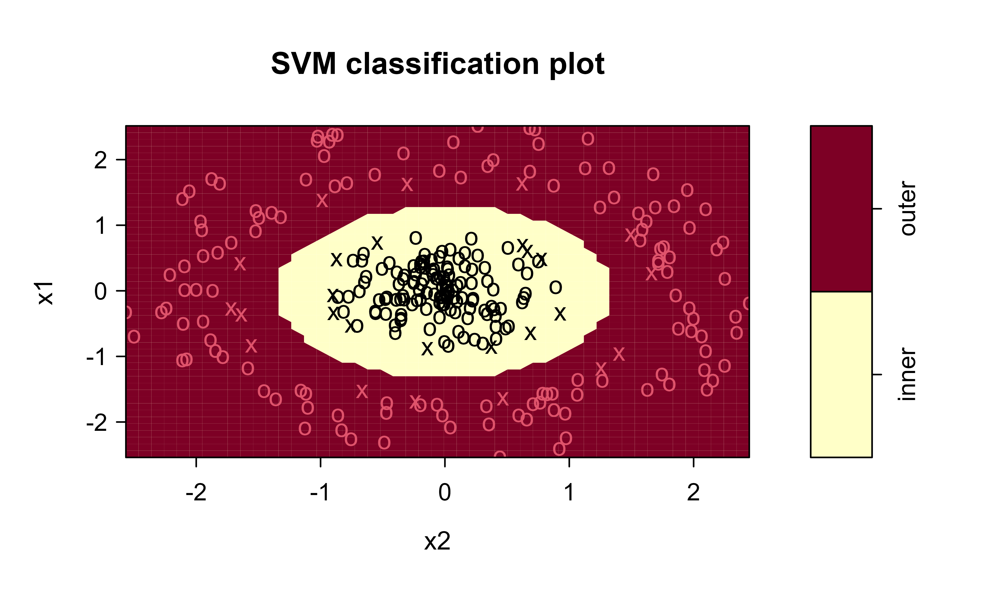
We need data that a straight line cannot separate, so generate an inner disk of one class surrounded by a ring of the other — the two-dimensional analogue of “no hyperplane will do”:
A linear kernel is restricted to a straight boundary; the radial basis function (RBF) kernel maps into an implicit infinite-dimensional space where the ring is linearly separable. The test accuracy tells the whole story:
The linear SVM is near chance because no line separates a disk from its surrounding ring; the RBF SVM is essentially perfect. Crucially, it never materializes the high-dimensional features — it only ever evaluates the kernel \(K(x_i, x_j)\) between points, which is the entire payoff of the dual formulation in Section 19.1.2.
RBF-kernel SVM decision regions; circled points are the support vectors that define the boundary.
19.5.2 Cost: the bias–variance dial
\(C\) governs how much the model pays for points inside the margin. Small \(C\) tolerates violations (a wide, smooth margin defined by many support vectors — higher bias); large \(C\) insists on classifying training points correctly (a narrow margin clinging to few support vectors — higher variance). Watch the support-vector count contract as \(C\) grows:
Because the support vectors are exactly the points on or inside the margin (Section 19.1.2), this count is the effective complexity of the fit — a model resting on 12 points generalizes differently from one resting on 100.
19.5.3 Tuning, honestly
\(C\) and the RBF width \(\gamma\) are not separable by eye; tune them jointly by cross-validation. tune() runs a 10-fold grid and returns the best cell:
The same machinery solves regression by fitting an \(\epsilon\)-insensitive tube (Equation 19.17): errors smaller than \(\epsilon\) cost nothing, so only points on or outside the tube become support vectors. On a noisy sine wave:
Show code
set.seed(1); x<-sort(runif(120, -3, 3)); y<-sin(x)+rnorm(120, 0, 0.2)svr<-svm(x, y, kernel ="radial", epsilon =0.1)sqrt(mean((predict(svr, x)-y)^2))# training RMSE#> [1] 0.1849076
The recurring practical lesson: the kernel encodes your assumption about shape, \(C\) and \(\epsilon\) encode your tolerance for error, and all three must be tuned rather than guessed. With a sensible kernel and cross-validated hyperparameters, the SVM is among the strongest off-the-shelf classifiers for small-to-medium tabular data.
19.6 Vector Quantization
We close with a related technique that shares the same geometric flavor of partitioning space into regions, but serves a different purpose: compression. Vector quantization (VQ) is used for image and voice compression (a form of lossy data compression) and for pattern recognition (source5). A few orienting remarks before the details:
VQ is part of the neural networks chapter (Chapter 15).
k-means clustering, covered in the cluster analysis chapter (Chapter 23), is itself a type of VQ.
Python currently has better tooling for VQ than R.
The core idea is to replace a continuous range of vectors with a small, fixed dictionary of representative vectors. Formally, a vector quantizer maps \(k\)-dimensional vectors in the vector space \(R^k\) into a finite set of vectors \(Y = \{ y_i, i = 1,\dots, N\}\). Each \(y_i\) is a code vector (or codeword), also known as a neuron in the language of the neural networks chapter (Chapter 15). The set of all codewords is a codebook, each attribute in the codebook is a weight, and the collection of codebook vectors forms a network.
Each codeword owns a region of space, namely the set of points closer to it than to any other codeword. This nearest-neighbor region is called a Voronoi region,
\[
V_i = \{ x \in R^k: ||x-y_i ||\le ||x - y_j|| \forall j \neq i \}
\]
Intuition
Think of the codewords as towns and the Voronoi regions as the surrounding areas whose residents live closer to that town than to any other. Every point in space belongs to exactly one town.
The Voronoi regions tile the whole space without gaps or overlaps. Formally they cover everything,
where \(x_j\) is the \(j\)th component of the input vector and \(y_{ij}\) is the \(j\)th component of the codeword \(y_i\). Prediction is made by searching through all codebook vectors for the most similar instances.
This structure gives a clean two-step compression scheme:
Encoder: map an input vector to the index of its nearest codeword.
Decoder: map a stored index back to the corresponding codeword.
Because we transmit or store only the small index instead of the full vector, we save space; the cost is that the reconstruction is the codeword rather than the exact input, which is why VQ is “lossy.”
The algorithm for building the codebook (Linde, Buzo, and Gray 1980) is closely related to the K-means algorithm covered in the cluster analysis chapter (Chapter 23). It shares K-means’s limitations, however: it is only locally optimal and can be quite slow.
Note
VQ performance is commonly assessed with either the Mean Squared Error (MSE) between inputs and their reconstructions, or the Peak Signal to Noise Ratio (PSNR), which expresses the same reconstruction quality on a decibel scale where higher is better.
Takeaways. Support vector methods all spring from one geometric idea, the widest separating slab, refined in stages: the maximal margin classifier finds the widest perfect separator; the support vector classifier softens it with a budget \(C\) for mistakes; the support vector machine bends the boundary using kernels; and the RKHS framework reveals all of this as a “loss plus penalty” problem whose infinite-dimensional setup collapses to a finite, support-vector-based solution. The same machinery extends to regression through an \(\epsilon\)-insensitive tube, and the partition-into-regions theme reappears in vector quantization for compression.
James, Gareth, Daniela Witten, Trevor Hastie, and Robert Tibshirani. 2013. “Statistical Learning.” In, 15–57. Springer New York. https://doi.org/10.1007/978-1-4614-7138-7_2.
Linde, Y., A. Buzo, and R. Gray. 1980. “An Algorithm for Vector Quantizer Design.”IEEE Transactions on Communications 28 (1): 84–95. https://doi.org/10.1109/tcom.1980.1094577.
Coding the two classes as \(-1\) and \(+1\) (rather than \(0\) and \(1\)) is a deliberate convenience: it lets us write the “correct side” condition as a single product \(y_i(\beta_0 + x_i^T\beta) > 0\), as we will see shortly.↩︎
Without the normalization you could make \(M\) arbitrarily large just by scaling up \(\beta\), which would be meaningless. Fixing \(||\beta|| = 1\) ties \(M\) to a genuine geometric distance.↩︎
The “reproducing” name comes exactly from this self-consistency. Evaluating a function in \(H_K\) at a point is the same as taking its inner product with the kernel centered at that point, so the kernel acts as a stand-in for point evaluation.↩︎
Both losses penalize confident wrong predictions heavily and confident correct predictions lightly. They differ mainly in that hinge loss flattens to exactly zero past the margin, while binomial deviance never quite reaches zero, which is what lets logistic regression produce calibrated probabilities.↩︎
# Support Vector {#sec-svm}```{r}#| include: falsesource("_common.R")```Suppose you have measurements on two groups of patients, healthy and sick, and you want a rule that takes a new patient's measurements and decides which group they belong to. One natural idea is to draw a boundary through the data and classify each new case by which side of the boundary it falls on. Support vector methods take this simple idea and push it as far as it will go: they look for the boundary that separates the classes with the widest possible buffer zone, and then, through a clever mathematical device, they let that boundary bend into curves and complicated shapes without paying the usual computational price.This chapter builds the idea up in layers. We start with the cleanest possible case, where the two classes can be split perfectly by a straight boundary, and we ask which straight boundary is best. That gives us the maximal margin classifier. Real data are rarely so cooperative, so we relax the rule to allow some mistakes, which gives the support vector classifier. We then ask how to draw curved boundaries, which leads us to support vector machines and the kernel trick, one of the most elegant ideas in machine learning. Along the way we connect everything to a general "loss plus penalty" view through reproducing kernel Hilbert spaces, which shows that support vector machines are one member of a much larger family. We close with two extensions: support vector regression for continuous outcomes, and vector quantization, a related compression technique.::: {.callout-tip title="Intuition"}The whole subject grows from one picture. Two clouds of points, and a stripe of empty space between them. Everything that follows is about how to find the widest stripe, what to do when the clouds overlap, and how to make the stripe curve.:::The mathematics here leans on geometry (hyperplanes, distances, inner products) and on convex optimization. You do not need to have seen these before; we define each term as it appears and give the picture before the formula.## Maximal Margin ClassifierWe begin in the friendliest setting, where the two classes can be separated cleanly. Suppose we have $n$ pairs of training data, $(x_1, y_1), \dots, (x_n, y_n)$, where each input $x_i \in R^p$ is a vector of $p$ measurements and each label $y_i \in \{-1, 1\}$ records which of two classes the observation belongs to.^[Coding the two classes as $-1$ and $+1$ (rather than $0$ and $1$) is a deliberate convenience: it lets us write the "correct side" condition as a single product $y_i(\beta_0 + x_i^T\beta) > 0$, as we will see shortly.]The object that does the separating is a hyperplane. A hyperplane in $p$-dimensional space is a "flat" affine subspace of dimension $p-1$. The word "flat" is doing real work here: a hyperplane has no curvature. If $p = 2$, the hyperplane is a line. If $p = 3$, the hyperplane is an ordinary plane. In higher dimensions we cannot picture it, but it behaves the same way.In two dimensions, a hyperplane is defined by the equation$$\beta_0 + \beta_1 X_1 + \beta_2 X_2 = 0$$so that any point $X_1, X_2$ that satisfies this equation lies on the hyperplane. In $p$ dimensions, the hyperplane is defined by$$\beta_0 + \beta_1 X_1 + \dots + \beta_p X_p = 0$$or equivalently, writing the predictors as a vector,$$\beta_0 + \mathbf{X}^T \beta = 0$$If the point $X = (X_1, \dots, X_p)^T$ does not lie on the hyperplane, it lies on one side or the other, which we can detect from the sign of the left-hand side:$$\beta_0 + X^T \beta >0 \\\beta_0 + X^T \beta <0$$The hyperplane therefore divides $p$-dimensional space into two half-spaces. To determine which side a point is on, we evaluate the sign of $\beta_0 + X^T \beta$, that is, $G(x) = \text{sign}[\beta_0 + X^T \beta]$.::: {.callout-important title="Key idea"}A linear classifier is nothing more than a hyperplane plus a sign rule. The sign tells you the predicted class; the value tells you how confident you should be.:::<br>Now we want to classify a new point $x^* = (x_1^*, \dots, x^*_p)^T$ using a separating hyperplane. To start, assume it is possible to construct a hyperplane that separates the training observations perfectly, with every positive-labeled point on one side and every negative-labeled point on the other. For the training data this means$$\begin{cases}\beta_0 + x_i^T \beta > 0 & \text{if } y_i = 1 \\\beta_0 + x_i^T \beta <0 & \text{if } y_i = -1\end{cases}$$These two cases combine neatly into a single statement. Because $y_i$ is $+1$ or $-1$, multiplying through by $y_i$ makes the product positive in both cases, so a separating hyperplane has the property$$y_i (\beta_0 + x_i^T \beta) >0$$for all $i = 1, \dots, n$. To classify $x^*$, we compute $f(x^*) = \beta_0 + \beta_1 x_1^* + \dots + \beta_p x_p^*$ and assign it to the first group if this is positive and to the second group if it is negative (this is exactly the rule $G(x)$ defined above). The magnitude of $f(x^*)$ tells us how far $x^*$ sits from the hyperplane, so larger magnitudes correspond to more confident classifications.At this point the separating hyperplane is simply a linear decision boundary. The catch is that when the classes are perfectly separable there are infinitely many such hyperplanes: you can nudge and tilt the boundary in countless ways and still keep every point on its correct side. We need a principle for choosing one.The natural principle is to pick the boundary that sits as far as possible from the data on both sides. We define an optimal separating hyperplane, also called the maximal margin hyperplane, as the hyperplane that is farthest from the training observations. To make this precise, measure the perpendicular distance from each observation to the hyperplane. The smallest of those distances is called the margin: it is the width of the empty buffer on either side of the boundary. The maximal margin hyperplane is the separating hyperplane with the largest margin, the one whose closest point is as far away as possible.::: {.callout-tip title="Intuition"}Imagine fitting the widest possible slab between the two classes, like sliding the thickest plank you can into the gap. The maximal margin hyperplane is the centerline of that plank.:::The classifier built from this hyperplane is the maximal margin classifier. The maximal margin hyperplane is the mid-line between the two classes that admits the widest "slab" we can insert between them.A small number of training points end up touching the edges of that slab, and these points are special. They are called support vectors: vectors in $p$-dimensional space that "support" the maximal margin hyperplane in the sense that if any of them moved, the hyperplane would move with it. Every other point is irrelevant to the boundary. As long as the non-support points do not cross the margin boundaries, they can move freely without changing the hyperplane at all. This property is what makes support vector methods both efficient and robust, and it carries over to support vector classifiers and support vector machines.We can find the maximal margin hyperplane by solving the following convex optimization problem,$$\underset{\beta_0,\dots, \beta_p}{\operatorname{max}} M$$subject to$$\sum_{j = 1}^p \beta_j^2 = 1$$that is, $||\beta|| = 1$, and$$y_i (\beta_0 + x_i^T \beta) \ge M,\forall i = 1, \dots, n$$Reading these pieces in plain language: the last constraint guarantees that every observation lands on the correct side of the hyperplane (provided $M$ is positive) with a cushion of at least $M$. The first constraint, the normalization $||\beta|| = 1$, fixes the scale so that the quantity $y_i (\beta_0 + x_i^T \beta)$ equals the actual perpendicular distance from the $i$-th observation to the hyperplane.^[Without the normalization you could make $M$ arbitrarily large just by scaling up $\beta$, which would be meaningless. Fixing $||\beta|| = 1$ ties $M$ to a genuine geometric distance.] Together they say: push every point at least a distance $M$ away from the boundary, and make $M$ as large as you can. The optimal $M$ is the margin.<br>### Why the margin equals $1/\|\beta\|$ {#sec-svm.qmd-margin-geom}The optimization above is stated with the constraint $\|\beta\| = 1$, which keeps $M$ equal to a genuine perpendicular distance. It is worth deriving that geometric fact, because it leads directly to the equivalent and more convenient formulation used in practice.Fix a hyperplane $\{x : \beta_0 + x^T\beta = 0\}$ with $\beta \neq 0$ (we do not yet impose $\|\beta\| = 1$). Take any point $x_0$ and let $x_p$ be its orthogonal projection onto the hyperplane. The vector $x_0 - x_p$ is parallel to the normal direction $\beta/\|\beta\|$, so $x_0 - x_p = t\,\beta/\|\beta\|$ for some scalar $t$ whose absolute value is the distance we want. Since $\beta_0 + x_p^T\beta = 0$,$$\beta_0 + x_0^T\beta = \beta_0 + (x_p + t\,\beta/\|\beta\|)^T\beta = \underbrace{(\beta_0 + x_p^T\beta)}_{=\,0} + t\,\frac{\beta^T\beta}{\|\beta\|} = t\,\|\beta\|.$$Hence the signed distance from $x_0$ to the hyperplane is$$\frac{\beta_0 + x_0^T\beta}{\|\beta\|},$$ {#eq-svm-signed-dist}and the functional margin $y_i(\beta_0 + x_i^T\beta)$ becomes the true geometric margin once divided by $\|\beta\|$. This is precisely why fixing $\|\beta\| = 1$ makes the constraint $y_i(\beta_0 + x_i^T\beta) \ge M$ read as "every point is at least geometric distance $M$ from the boundary."The normalization $\|\beta\| = 1$ is awkward for an optimizer because it is a nonconvex equality constraint. We can remove it by a standard reparameterization. Drop $\|\beta\| = 1$ and instead require, from @eq-svm-signed-dist,$$\frac{1}{\|\beta\|}\, y_i(\beta_0 + x_i^T\beta) \ge M, \qquad i = 1, \dots, n.$$The hyperplane is unchanged if we rescale $(\beta_0, \beta)$ by any positive constant, so we are free to fix that scale by setting $\|\beta\| = 1/M$, which turns the constraints into $y_i(\beta_0 + x_i^T\beta) \ge 1$. Maximizing $M$ is then the same as minimizing $\|\beta\|$, or equivalently $\tfrac{1}{2}\|\beta\|^2$, giving the canonical convex program$$\min_{\beta_0, \beta} \ \frac{1}{2}\|\beta\|^2 \quad \text{subject to} \quad y_i(\beta_0 + x_i^T\beta) \ge 1, \ i = 1, \dots, n.$$ {#eq-svm-primal-hard}This is a quadratic program with a strictly convex objective and linear inequality constraints, so it has a unique solution. The margin width recovered from the optimum is $2/\|\hat\beta\|$ (the distance $1/\|\hat\beta\|$ on each side).### The Lagrangian dual and support vectors {#sec-svm.qmd-dual}The dual of @eq-svm-primal-hard is where the support vectors and, later, the kernel trick come from, so we derive it in full. Introduce one multiplier $\alpha_i \ge 0$ per constraint and form the Lagrangian$$\mathcal{L}(\beta_0, \beta, \alpha) = \frac{1}{2}\|\beta\|^2 - \sum_{i=1}^n \alpha_i\big[y_i(\beta_0 + x_i^T\beta) - 1\big].$$ {#eq-svm-lagrangian}Setting the partial derivatives to zero gives the stationarity conditions$$\frac{\partial \mathcal{L}}{\partial \beta} = \beta - \sum_{i=1}^n \alpha_i y_i x_i = 0 \ \Rightarrow\ \beta = \sum_{i=1}^n \alpha_i y_i x_i, \qquad\frac{\partial \mathcal{L}}{\partial \beta_0} = -\sum_{i=1}^n \alpha_i y_i = 0.$$ {#eq-svm-stationary}Substituting $\beta = \sum_i \alpha_i y_i x_i$ back into @eq-svm-lagrangian and using $\sum_i \alpha_i y_i = 0$ to kill the $\beta_0$ term, the quadratic term becomes $\tfrac12\sum_{i,i'}\alpha_i\alpha_{i'}y_iy_{i'}x_i^Tx_{i'}$ and the linear term contributes $-\sum_{i,i'}\alpha_i\alpha_{i'}y_iy_{i'}x_i^Tx_{i'} + \sum_i\alpha_i$, leaving the Wolfe dual$$\max_{\alpha} \ \sum_{i=1}^n \alpha_i - \frac{1}{2}\sum_{i=1}^n\sum_{i'=1}^n \alpha_i \alpha_{i'} y_i y_{i'} \, x_i^T x_{i'}\quad \text{s.t.} \quad \alpha_i \ge 0, \ \sum_{i=1}^n \alpha_i y_i = 0.$$ {#eq-svm-dual-hard}Two features of @eq-svm-dual-hard are decisive. First, the data enter only through the inner products $x_i^T x_{i'}$; nowhere do we need the raw coordinates. This is exactly the opening through which the kernel trick later enters, by replacing $x_i^T x_{i'}$ with $K(x_i, x_{i'})$. Second, the Karush-Kuhn-Tucker (KKT) complementary slackness condition$$\alpha_i\big[y_i(\beta_0 + x_i^T\beta) - 1\big] = 0$$ {#eq-svm-kkt}forces $\alpha_i = 0$ for every point strictly outside the margin (where $y_i(\beta_0 + x_i^T\beta) > 1$). Only points lying exactly on the margin, where $y_i(\beta_0 + x_i^T\beta) = 1$, can have $\alpha_i > 0$. These are the support vectors, and by @eq-svm-stationary the solution $\hat\beta = \sum_{i\in S}\hat\alpha_i y_i x_i$ depends on them alone. This is the algebraic origin of the "only the support vectors matter" property asserted geometrically above. The offset is recovered from any margin point $i$ with $\hat\alpha_i > 0$ via $\hat\beta_0 = y_i - x_i^T\hat\beta$, usually averaged over all support vectors for numerical stability.This clean story has limits. The method breaks down if no separating hyperplane exists, that is, if no flat boundary can split the two classes. And even when a perfect separator does exist, it may not be the boundary we want. There are two situations where insisting on perfect separation is a bad idea:1. The separating hyperplane has a very small margin, so the classifier is barely committed to either class near the boundary.2. The boundary is very sensitive to one or two observations, in which case it will most likely overfit and generalize poorly.::: {.callout-warning}Perfect separation on the training data is not the goal. A boundary that threads perfectly between every training point is often one that has memorized noise. The next section trades a little training accuracy for a lot of stability.:::<br>## Support Vector ClassifiersThe two problems just raised motivate a more forgiving classifier, one based on a hyperplane that does not perfectly separate the classes. Accepting a few mistakes buys us two things:1. greater robustness to individual observations, and2. better classification of most of the training observations.Such a soft margin classifier is the support vector classifier. It is constructed much like the maximal margin classifier, except that we now allow some observations to fall on the wrong side of the margin, or even on the wrong side of the hyperplane itself. The phrase "soft margin" captures the idea: the buffer zone is no longer an inviolable wall but a soft boundary that a few points may cross.Implementing a support vector classifier is again an optimization problem, obtained by modifying one constraint of the maximal margin problem and adding another. The support vector classifier is given by the solution to$$\underset{\beta_0,\dots, \beta_p, \epsilon_1, \dots, \epsilon_n}{\operatorname{max}} M$$subject to$$\sum_{j=1}^p \beta_j^2 = 1$$(that is, $||\beta|| = 1$) and$$y_i (\beta_0 + x_i^T \beta) \ge M(1 - \epsilon_i), \forall i = 1, \dots, n$$$$\epsilon_i \ge 0, \sum_{i=1}^n \epsilon_i \le C$$where $C$ is a non-negative tuning parameter and $M$ is the margin.The new ingredients are the $\epsilon_i, i = 1, \dots, n$, called slack variables. Each $\epsilon_i$ measures how much observation $i$ is allowed to violate the margin, giving the model the flexibility to place a point on the wrong side of the margin or even the hyperplane. As before, we classify a new observation $x^*$ via the sign of $f(x^*)$.The slack variables tell a readable story about where each observation sits relative to the margin:- $\epsilon_i = 0$ means the point is on the correct side of the margin.- $\epsilon_i >0$ means the point is on the wrong side of the margin.- $\epsilon_i >1$ means the point is on the wrong side of the hyperplane (a true misclassification).The tuning parameter $C$ ties these violations together. Since $C$ is the upper bound on the sum of the $\epsilon_i$, it determines the number and severity of the violations we will tolerate. You can think of $C$ as a budget for the total amount by which the margin may be violated across all $n$ observations [@james2013, p. 376].The two extremes are worth holding in mind. If $C = 0$, there is no budget for violations, so every $\epsilon_i = 0$, and we are back to the [Maximal Marginal Classifier] (assuming the classes are separable). If $C >0$, no more than $C$ observations can be on the wrong side of the hyperplane, since each such observation contributes $\epsilon_i > 1$. As $C$ increases, we tolerate more violations, and the margin widens to accommodate them.::: {.callout-important title="Key idea"}$C$ is the dial that controls the bias-variance trade-off for a support vector classifier, and it is usually chosen by cross-validation.:::Turning that dial in either direction has predictable effects:- $C$ small: narrow margins, few margin violations, low bias, high variance, and fewer support vectors.- $C$ large: wide margins, more violations, more bias but less variance, and many support vectors.As before, the support vectors are the observations that lie on or inside the margins. Because the decision rule depends only on this relatively small set of points, the support vector classifier is robust to the behavior of observations far from the hyperplane. This is a real contrast with linear discriminant rules (see @sec-discriminant-analysis), which let every observation, even distant ones, pull on the boundary.### The soft-margin program and its dual {#sec-svm.qmd-soft-dual}The textbook formulation above measures the budget $C$ in units of margin width, which is geometric but inconvenient for solvers. The equivalent and far more common form, the one implemented in `e1071`, `kernlab`, and LIBSVM, applies the rescaling of @sec-svm.qmd-margin-geom (set $\|\beta\| = 1/M$, write $\xi_i = M\epsilon_i$) to obtain a convex quadratic program in standardized slacks $\xi_i \ge 0$:$$\min_{\beta_0, \beta, \xi} \ \frac{1}{2}\|\beta\|^2 + C\sum_{i=1}^n \xi_i\quad \text{s.t.} \quad y_i(\beta_0 + x_i^T\beta) \ge 1 - \xi_i, \ \ \xi_i \ge 0.$$ {#eq-svm-primal-soft}::: {.callout-warning title="Two meanings of C"}The cost $C$ in @eq-svm-primal-soft is not the budget $C$ of the geometric formulation; the two are inversely related. In @eq-svm-primal-soft a large $C$ heavily penalizes violations and yields a narrow, hard margin, whereas in the budget formulation a large $C$ permits more violations and a wider margin. Software almost always uses the cost convention of @eq-svm-primal-soft, so read the documentation before tuning.:::The dual is derived as before. With multipliers $\alpha_i \ge 0$ on the margin constraints and $\mu_i \ge 0$ on $\xi_i \ge 0$, stationarity in $\xi_i$ gives $C - \alpha_i - \mu_i = 0$, hence $0 \le \alpha_i \le C$. The other stationarity conditions are identical to @eq-svm-stationary, and the dual is the same objective as the separable case but with a box constraint:$$\max_{\alpha} \ \sum_{i=1}^n \alpha_i - \frac{1}{2}\sum_{i,i'} \alpha_i \alpha_{i'} y_i y_{i'}\, x_i^T x_{i'}\quad \text{s.t.} \quad 0 \le \alpha_i \le C, \ \sum_{i=1}^n \alpha_i y_i = 0.$$ {#eq-svm-dual-soft}The KKT conditions now sort the points into three groups, which is the most useful diagnostic the dual offers. From $\alpha_i[y_i f(x_i) - 1 + \xi_i] = 0$ and $\mu_i \xi_i = (C - \alpha_i)\xi_i = 0$:- $\alpha_i = 0$: the point is strictly outside the margin ($y_i f(x_i) > 1$), not a support vector;- $0 < \alpha_i < C$: then $\xi_i = 0$ and $y_i f(x_i) = 1$, a margin support vector lying exactly on the margin (these are used to solve for $\hat\beta_0$);- $\alpha_i = C$: then $\xi_i \ge 0$ and the point is inside the margin or misclassified, a bound support vector.The fraction of points with $\alpha_i = C$ is a direct read on how aggressively the budget is being spent. The closely related $\nu$-SVM reparameterizes $C$ as $\nu \in (0,1]$, which bounds the fraction of margin errors from above and the fraction of support vectors from below, giving the tuning parameter a concrete interpretation.## Nonlinear Decision BoundariesSo far every boundary has been flat. Many problems, though, call for a curved one. A simple way to get curvature is to enrich the feature set. Instead of fitting a support vector classifier using only the $p$ features $X_1, \dots, X_p$, we add their squares and work with $2p$ features (linear and quadratic terms),$$X_1, X_1^2, \dots, X_p, X^2_p$$The optimization problem then becomes$$\underset{\beta_0,\dots, \beta_p, \epsilon_1, \dots, \epsilon_n}{\operatorname{max}} M$$subject to$$y_i (\beta_0 + \sum_{j=1}^p \beta_{j1}x_{ij} + \sum_{j=1}^p \beta_{j2} x_{ij}^2) \ge M (1 - \epsilon_i), \forall i = 1, \dots, n$$$$\epsilon_i \ge 0 , \sum_{i=1}^n \epsilon_i \le C, \sum_{j = 1}^p \sum_{k = 1}^2 \beta_{jk}^2 = 1$$Here is the trick that makes this so useful. The boundary is nonlinear (quadratic) in the original feature space, but it is perfectly linear in the expanded $2p$-dimensional space. We have not invented a new algorithm; we have run the same linear machinery in a bigger space and let the extra dimensions carry the curvature.::: {.callout-tip title="Intuition"}Lift the data into a higher-dimensional space where a flat cut suffices, make the flat cut there, then project the cut back down. What looks like a straight slice upstairs looks like a curve downstairs.:::Once we accept this idea, nothing stops us from going further: we could add cubic terms, higher polynomials, interactions, or any other functions (for example, spline-style basis functions) of the predictors. The difficulty is that there are infinitely many choices, and naively expanding the feature space quickly becomes computationally impossible. The support vector machine provides a principled way to enlarge the feature space while keeping the computation tractable. Two facts make this possible:1. Only the support vectors matter for determining the classification boundary.2. A kernel representation lets us work in the enlarged space without ever constructing it explicitly.The next section develops the second of these, which is the heart of the matter.<br>## Support Vector MachinesThe support vector machine (SVM) is an extension of the [Support Vector Classifiers] that enlarges the feature space using transformations of the inputs called kernels. The payoff is flexible, curved decision boundaries with the same efficient optimization as before.To set up the idea, consider a collection of $m$ basis functions of the features $x$,$$h(x_i) = (h_1(x_i), h_2(x_i), \dots, h_m (x_i))^T, i = 1, \dots, n$$We could then use the [Support Vector Classifiers] machinery to find parameters $\hat{\beta}$ in $f(x) = \beta_0 + h(x)^T \beta$, and classify by $\hat{G}(x) = \text{sign} (\hat{f}(x))$. This raises an obvious question: how do we choose the basis functions $h$?The remarkable answer is that we do not have to choose them at all. It is enough to choose a positive definite kernel function $K(x_i, x_{i'})$, and that single choice implicitly determines a whole collection of basis functions. The same positive definite kernels underpin Gaussian process regression (@sec-gaussian-process-reg), which offers a probabilistic counterpart to the kernel machinery developed here. To see why, we first need to recall inner products.::: {.callout-note}The kernel does double duty. It encodes a similarity between two observations, and it secretly stands in for an inner product in some (possibly enormous) feature space. The "trick" is that we get the second for free once we specify the first.:::An inner product of two $r$-dimensional vectors $a$ and $b$ is $<a,b> = \sum_{j=1}^r a_j b_j$, a single number that measures how aligned the two vectors are. For two inputs $x_i$ and $x_i'$ this is$$<x_i, x_i'> = \sum_{j= 1}^p x_{ij} x_{i'j}$$The key fact is that a positive definite kernel can be written as the inner product of some set of basis functions:$$K(x_i, x_{i'}) = < h(x_i), h(x_{i'})>$$This is easiest to appreciate through an example. Take the second-degree polynomial kernel$$K(x, \tilde{x}) = (1 + <x, \tilde{x}>)^2$$with $p = 2$, so $x = (x_1, x_2)$ and $\tilde{x} = (\tilde{x}_1, \tilde{x}_2)$. Expanding the square,$$\begin{aligned}K(x, \tilde{x}) &= (1 + < x, \tilde{x}>)^2 \\& = (1 + x_1 \tilde{x}_1 + x_2 \tilde{x}_2)^2 \\&= 1 + 2 x_1 \tilde{x}_1 + 2 x_2 \tilde{x}_2 + (x_1 \tilde{x}_1)^2 + (x_2 \tilde{x}_2)^2 + 2 x_1 \tilde{x}_1 x_2 \tilde{x}_2\end{aligned}$$If we match this against $K(x, \tilde{x}) = <h(x), h(\tilde{x})>$, we can read off $m = 6$ basis functions:$$h_1(x) = 1 \\h_2(x) = \sqrt{2}x_1 \\h_3(x) = \sqrt{2}x_2 \\h_4 (x) = x_1^2 \\h_5 (x) = x_2^2 \\h_6(x) = \sqrt{2} x_1 x_2$$Notice what just happened: by evaluating one simple kernel, we implicitly worked in a six-dimensional feature space without ever writing those six features down. This is the powerful idea behind regularized (penalized) modeling known as Reproducing Kernel Hilbert Spaces (RKHS), which we develop next.### When is a function a valid kernel? {#sec-svm.qmd-mercer}We have been asserting that a "positive definite kernel" can be written as an inner product $K(x,\tilde x) = \langle h(x), h(\tilde x)\rangle$. That assertion is not free; it is the content of Mercer's theorem, and the condition it requires is exactly what must be checked before a candidate similarity function may be used in @eq-svm-dual-soft.A symmetric function $K$ is a (positive semdefinite) kernel if for every finite set $x_1, \dots, x_n$ the Gram matrix $\mathbf{K}$ with entries $K_{ii'} = K(x_i, x_{i'})$ satisfies$$c^T \mathbf{K} c = \sum_{i=1}^n\sum_{i'=1}^n c_i c_{i'} K(x_i, x_{i'}) \ge 0 \qquad \text{for all } c \in \mathbb{R}^n.$$ {#eq-svm-psd}This condition matters operationally for two reasons. First, it is exactly what makes the dual objective @eq-svm-dual-soft concave (the Gram matrix is the Hessian, so positive semidefiniteness guarantees a single global optimum). Second, it certifies that an implicit feature map exists, so the geometric picture of a separating hyperplane in feature space is legitimate. A useful calculus follows from @eq-svm-psd: sums of kernels, positive scalar multiples, products, and limits of kernels are again kernels, which is how one verifies the radial basis kernel $\exp(-\gamma\|x-\tilde x\|^2)$ from the simpler building blocks. The neural network ("sigmoid") kernel $\tanh(\kappa_1\langle x,\tilde x\rangle + \kappa_2)$ is the cautionary case: it fails @eq-svm-psd for many parameter values, so its Gram matrix can be indefinite and the dual loses its convexity guarantee.We can verify the kernel-equals-inner-product identity numerically. The chunk below computes the degree-2 polynomial kernel directly and via the six explicit basis functions $h(x)$ derived above, and confirms they agree, and separately checks that an RBF Gram matrix satisfies the positive-semidefiniteness condition @eq-svm-psd (all eigenvalues nonnegative).```{r}#| label: svm-kernel-checkset.seed(1)x <-runif(2); xt <-runif(2) # two points in R^2h <-function(z) c(1, sqrt(2)*z[1], sqrt(2)*z[2], z[1]^2, z[2]^2, sqrt(2)*z[1]*z[2])c(kernel = (1+sum(x*xt))^2, feature_inner =sum(h(x)*h(xt)))X <-matrix(runif(20*3), 20, 3) # 20 points in R^3D <-as.matrix(dist(X))^2K <-exp(-0.5* D) # RBF Gram matrixmin(eigen(K, symmetric =TRUE, only.values =TRUE)$values) # >= 0 (up to rounding)```### Regularization by RKHSThis section [@hastie2001a, 5.8] places the SVM inside a much broader framework. The reward for the extra abstraction is a single result that covers many methods at once: it shows that an apparently infinite-dimensional problem collapses to a finite one.The general regularization (penalized loss) problem is$$\underset{f \in H}{\operatorname{min}} [ \sum_{i = 1}^n L(y_i, f(x_i)) + \lambda J(f)]$$ {#eq-svm-reg1}where the three pieces are- $L(y_i, f(x_i))$, the loss function, which penalizes poor fit;- $J(f)$, a penalty function, which penalizes complicated functions; and- $H$, a space of functions on which $J(f)$ is defined.To specialize this to kernels, consider a positive definite kernel $K(x, \tilde{x})$ for $x, \tilde{x} \in R^p$ with an eigen-expansion$$K(x, \tilde{x}) = \sum_{j=1}^\infty \delta_j \phi_j(x) \phi_j (\tilde{x})$$with eigenvalues $\delta_j >0, \sum_{j = 1}^\infty \delta^2_j < \infty$ and eigenfunctions $\{ \phi_j (.)\}$. The idea is to use these eigenfunctions as our basis functions, and to look for functions $f(x)$ expressed in terms of them,$$f(x) = \sum_{j=1}^\infty c_j \phi_j (x)$$subject to the constraint that $J(f) = ||f||^2_{H_K} \equiv \sum_{j=1}^\infty c_j^2/\delta_j < \infty$. This function space, $H_K$, is called a reproducing kernel Hilbert space because the kernel reproduces itself under the inner product: $<K(.,x_i), K(x,x_{i'})> = K(x_i, x_{i'})$.^[The "reproducing" name comes exactly from this self-consistency. Evaluating a function in $H_K$ at a point is the same as taking its inner product with the kernel centered at that point, so the kernel acts as a stand-in for point evaluation.]Substituting the eigenfunction expansion into the general problem rewrites the regularization problem as$$\underset{\{c_j\}^\infty_1}{\operatorname{min}} [\sum_{i=1}^nL(y_i, \sum_{j = 1}^\infty c_j \phi_j (x_i)) + \lambda \sum_{j = 1}^\infty \frac{c_j^2}{\delta_j} ]$$ {#eq-svm-reg2}At first glance this looks worse, since we now appear to have an infinite number of coefficients $c_j$ to estimate. The central result of RKHS theory is that, despite appearances, the solution is finite. It can be shown to take the form$$f(x) = \sum_{i=1}^n \alpha_i K(x, x_i)$$with a finite penalty$$J(f) = \sum_{i=1}^n \sum_{j=1}^n K(x_i, x_j) \alpha_i \alpha_j$$::: {.callout-important title="Key idea"}Although the optimization is set up over an infinite-dimensional space of functions, the solution is finite-dimensional, indexed by the $n$ training points. This is the **kernel trick**, and it is what makes kernel methods usable in practice.:::This is the representer theorem, and the argument behind it is short enough to give. Any $f \in H_K$ can be split into a part lying in the span of the kernel sections at the training points and a part orthogonal to it,$$f = \sum_{i=1}^n \alpha_i K(\cdot, x_i) + g, \qquad \langle g, K(\cdot, x_i)\rangle_{H_K} = 0 \ \text{ for all } i.$$By the reproducing property $f(x_i) = \langle f, K(\cdot, x_i)\rangle_{H_K}$, the orthogonal part $g$ contributes nothing to any fitted value $f(x_i)$, hence nothing to the loss term $L(y_i, f(x_i))$. But $g$ does inflate the penalty, since by the Pythagorean identity $\|f\|^2_{H_K} = \|\sum_i \alpha_i K(\cdot,x_i)\|^2_{H_K} + \|g\|^2_{H_K}$. Because the penalty $J(f) = \|f\|^2_{H_K}$ is strictly increasing, the minimizer must take $g = 0$. The optimum therefore lies in the $n$-dimensional span $\{K(\cdot, x_i)\}_{i=1}^n$ regardless of how large the underlying space $H_K$ is. This is what reduces the infinite program @eq-svm-reg2 to the finite program @eq-svm-reg3.In fact, the infinite-dimensional problem reduces to the finite-dimensional optimization$$\underset{\alpha}{\operatorname{min}} [ L(\mathbf{y}, \mathbf{K\alpha})+ \lambda \mathbf{\alpha}^T \mathbf{K \alpha}]$$ {#eq-svm-reg3}where $\mathbf{K}$ is the matrix with $(i,j)$th entry $K(x_i, x_j)$. The strength of this result is its generality: it works for any convex loss function and any positive definite kernel. The chain of reformulations from @eq-svm-reg1 to @eq-svm-reg2 to @eq-svm-reg3 turns a hard, abstract problem into a concrete one you can hand to an optimizer.This connects directly back to [Support Vector Machines]. To recover the SVM, all we need is the right loss function plus a positive definite kernel. The loss function associated with the support vector classifier turns out to be $[1 - y_i f(x_i)]_+$, where the "+" denotes the positive part of the bracketed quantity. This is called hinge loss: it charges nothing once a point is comfortably on the correct side of the margin, and charges a growing penalty as a point moves the wrong way.Then the solution to the constrained minimization$$\underset{\beta_0, \beta}{\operatorname{min}} [ \sum_{i=1}^n [1 - y_i f(x_i)]_+ + \frac{\lambda}{2}||\beta||^2]$$ {#eq-svm-reg4}gives the same estimates for $\beta$ as the support vector classifier, where $\lambda$ is proportional to $C$ as before. To express this in terms of the kernel's basis functions, suppose the basis set $\{ h_j(x) \}$ comes from the eigen-decomposition $K(x, \tilde{x}) = \sum_{j = 1}^\infty \delta_j \phi_j (x) \phi_j (\tilde{x})$, so that $h_j(x) = \sqrt{\delta_j} \phi_j(x)$. Letting $\theta_j \equiv \sqrt{\delta_j}\, \beta_j$ (recall the desired function is an expansion in these basis functions), the minimization becomes$$\underset{\beta_0, \theta}{\operatorname{min}} [ \sum_{i=1}^n [1 - y_i (\beta_0 + \sum_{j=1}^\infty \theta_j \phi_j(x_i))]_+ + \frac{\lambda}{2} \sum_{j=1}^\infty \frac{\theta_j^2}{\delta_j}]$$ {#eq-svm-reg5}One strength of the RKHS view of the SVM is that the "loss plus penalty" form makes it simple to swap in any convex loss function. For instance, using logistic regression as a classifier behaves much like an SVM, because the binomial deviance loss is shaped similarly to the hinge loss.^[Both losses penalize confident wrong predictions heavily and confident correct predictions lightly. They differ mainly in that hinge loss flattens to exactly zero past the margin, while binomial deviance never quite reaches zero, which is what lets logistic regression produce calibrated probabilities.] The RKHS theory then delivers the finite-dimensional solution @eq-svm-reg3, $f(x) = \beta_0 + \sum_{i=1}^n \alpha_i K(x, x_i)$, which equivalently minimizes$$\underset{\beta_0, \alpha}{\operatorname{min}} [ \sum_{i=1}^n [1 - y_i f(x_i)]_+ + \frac{\lambda}{2} \mathbf{\alpha}^T \mathbf{K \alpha}]$$ {#eq-svm-reg6}As a sanity check, choose a linear kernel, $K(x, x_i) = <x, x_i>$ (which is the ordinary Euclidean inner product, proportional to cosine similarity only after centering and normalizing). The solution becomes $f(x) = \beta_0 + \sum_{i=1}^n \alpha_i <x, x_i>$, which is exactly the [Support Vector Classifiers]. The linear kernel recovers the linear model, as it should.For genuine SVM analysis we usually pick a richer kernel to allow flexible boundaries. The common choices are:- the $d$-th degree polynomial kernel, $K(x, \tilde{x}) = (1 + <x, \tilde{x}>)^d$;- the radial basis kernel (effectively Gaussian), $K(x, \tilde{x}) = \exp(-\gamma ||x - \tilde{x}||^2 )$; and- the neural network kernel, $K(x, \tilde{x}) = \tanh (\kappa_1 <x, \tilde{x}>+ \kappa_2)$.::: {.callout-tip title="When to use this"}The radial basis kernel is the usual default when you have no strong prior knowledge about the shape of the boundary, since it can approximate a wide range of curved boundaries from local information. Reach for a polynomial kernel when you expect interactions up to a known degree.:::The honest drawback is that there is no general rule telling you which kernel to pick; the choice is typically made by cross-validation.The finite-dimensional kernel representation also pays off computationally. We only need to consider the $\binom{n}{2}$ distinct pairs of $x_i$ and $x_{i'}$ in the kernel matrix. That can still be a large number, but it is finite, which is a decisive improvement over the infinite-dimensional feature space we started from. A second economy comes from sparsity: $\alpha_i = 0$ whenever the feature vector $x_i$ is not a support vector. This holds because the hinge loss is exactly zero for observations with $y_i f(x_i) \ge 1$, which are the ones safely on the correct side of the margin. The solution therefore simplifies to$$f(x) = \beta_0 + \sum_{i \in S} \alpha_i K(x, x_i)$$where $S$ is the set of support vectors. It can further be shown that for a given $\lambda$, $\beta = (1/\lambda) \sum_{i \in S} \alpha_i y_i x_i$.::: {.callout-tip}Because only support vectors carry nonzero $\alpha_i$, a fitted SVM stores and uses just those points at prediction time. Counting the support vectors is a quick diagnostic: a model that turns most observations into support vectors is fitting a very wiggly boundary and may be overfit.:::### Theoretical properties and what they cost {#sec-svm.qmd-properties}A few facts give the SVM its place among classifiers and set expectations for cost and behavior.The hinge loss is a calibrated surrogate. Its population minimizer is $f^\star(x) = \operatorname{sign}(2\eta(x) - 1)$, where $\eta(x) = \Pr(Y=1\mid x)$, so the SVM decision rule targets the Bayes classifier directly. The price for the sparsity it buys is that, unlike logistic loss, the hinge loss does not recover the conditional probability $\eta(x)$ itself, only the sign of $2\eta(x)-1$; this is why a fitted SVM gives a decision but not a calibrated probability without an extra step such as Platt scaling.Margin theory, not dimension, controls generalization. Classical VC bounds for linear classifiers degrade with the feature-space dimension, which would be fatal for kernels that map into infinite-dimensional spaces. The relevant guarantee instead bounds the expected error by a quantity of order $R^2/(M^2 n)$, where $R$ bounds $\|x\|$ in feature space and $M$ is the achieved margin. Because the bound depends on the margin and not the ambient dimension, a high-dimensional kernel embedding does not by itself cause overfitting, which is the theoretical explanation for the SVM's empirical robustness in $p \gg n$ settings.Computational cost is the main practical limit. Forming the Gram matrix is $O(n^2 p)$ in time and the matrix itself is $O(n^2)$ in memory, and solving the dual QP is between $O(n^2)$ and $O(n^3)$ depending on the number of support vectors. Decomposition methods such as SMO (sequential minimal optimization), which repeatedly optimizes the dual over a pair of $\alpha_i$ analytically, make this tractable, but kernel SVMs still scale poorly past roughly $10^4$ to $10^5$ observations. For large $n$ with a linear kernel, primal solvers (for example LIBLINEAR) run in roughly $O(np)$ and are far faster; for nonlinear kernels, low-rank Nystrom or random-feature approximations of $\mathbf{K}$ are the standard escape. Prediction costs $O(|S|\,p)$ per query, so a model with many support vectors is slow at test time as well as a sign of overfitting.Failure modes. The kernel SVM degrades when features are on wildly different scales (the radial kernel is dominated by the largest-variance coordinate, so standardize inputs first), when $\gamma$ is too large (the radial kernel becomes a near-nearest-neighbor rule that memorizes the training set), and when classes are severely imbalanced (a single global $C$ lets the majority class dominate; per-class weights $C_+ , C_-$ are the fix).### Choosing the kernel and its hyperparameters {#sec-svm.qmd-howto}For the radial basis kernel the two knobs are the cost $C$ of @eq-svm-primal-soft and the bandwidth $\gamma$, and they interact, so they must be tuned jointly on a two-dimensional grid by cross-validation rather than one at a time. A geometric (logarithmic) grid is standard, for example $C \in \{2^{-5}, \dots, 2^{15}\}$ and $\gamma \in \{2^{-15}, \dots, 2^{3}\}$. A useful default scale for $\gamma$ is the inverse of the median squared pairwise distance between training points (the "median heuristic"), which gives a sensible starting point before refining the grid. Always standardize features before fitting an RBF SVM.::: {.callout-tip title="Practical recipe"}Standardize inputs; start from the median-heuristic $\gamma$ and $C = 1$; cross-validate on a log-spaced $(C, \gamma)$ grid; then inspect the support-vector fraction. If nearly every point is a support vector, $\gamma$ is too large or $C$ too small and the boundary is overfit; if very few points are, the boundary may be too rigid.:::Alternative Loss Functions. The hinge loss is not the only sensible choice. One useful alternative is the Huberized loss, which blends the attractive features of two worlds: it keeps the support-point sparsity of the hinge loss while staying smooth like logistic regression (so you can estimate probabilities), and it behaves well in the presence of outliers.Extensions to Multiple Classes. Everything above assumed two classes. Extending the SVM to more than two is not obvious, because the notion of a single separating hyperplane does not generalize cleanly beyond the binary case. Two standard work-arounds reduce the multiclass problem to many binary problems. The one-versus-one approach, for $K > 2$ classes, fits $\binom{K}{2}$ SVMs, one for each pair of classes. Given a new observation, every classifier votes, and the class chosen most often wins. The one-versus-all approach (often preferable) instead fits $K$ SVMs, each comparing one class against all the others, producing $K$ functions $f_k(x), k = 1, \dots, K$. For a test observation $x^*$ we choose the class $k$ for which $f_k(x^*)$ is largest. Given that logistic regression gives results similar to SVMs in the binary case, a multinomial-logistic classifier (using a multinomial loss function) may in fact be a better route to classification when $K>2$.### SVM RegressionThe same "loss plus penalty" paradigm extends naturally from classification to continuous responses, giving support vector machine regression. We again seek coefficients $\beta$ in $f(x) = \beta_0 + x^T \beta$, but now relative to a loss suited to a numeric outcome. To keep the spirit of the margin, we want a loss where only residuals larger in absolute value than some positive constant $\epsilon$ contribute, leaving a "tube" of width $\epsilon$ around the fit inside which errors cost nothing:$$\underset{\beta_0, \beta}{\operatorname{min}} [ V_\epsilon (y_i - f(x_i)) + \frac{\lambda}{2}||\beta||^2]$$where$$V_\epsilon(r) \equiv\begin{cases}0, & \text{if } |r| < \epsilon \\|r|- \epsilon, & \text{otherwise}\end{cases}$$so that errors smaller than $\epsilon$ are ignored [@hastie2001a, 12.3.6].::: {.callout-tip title="Intuition"}In classification the margin is a buffer between classes; in regression the analogous buffer is a tube around the regression line. Points inside the tube are "close enough" and contribute nothing to the loss, so only points outside the tube act as support vectors.:::This $\epsilon$-insensitive loss resembles other robust regression losses, such as the Huber loss, in that it limits the influence of moderate errors and keeps the fit from chasing every point.To turn the tube into an optimization the solver can handle, split each residual into a part above the tube and a part below it using two nonnegative slacks $\xi_i, \xi_i^\ast$, giving the primal$$\min_{\beta_0,\beta,\xi,\xi^\ast} \ \frac{1}{2}\|\beta\|^2 + C\sum_{i=1}^n(\xi_i + \xi_i^\ast)\quad \text{s.t.} \quad\begin{cases}y_i - f(x_i) \le \epsilon + \xi_i,\\f(x_i) - y_i \le \epsilon + \xi_i^\ast,\\\xi_i, \xi_i^\ast \ge 0.\end{cases}$$ {#eq-svm-svr-primal}The same Lagrangian steps as in @sec-svm.qmd-dual, now with multipliers $\alpha_i, \alpha_i^\ast \in [0, C]$ on the two constraint families, give the dual$$\max_{\alpha,\alpha^\ast} \ -\frac{1}{2}\sum_{i,i'}(\alpha_i-\alpha_i^\ast)(\alpha_{i'}-\alpha_{i'}^\ast)K(x_i,x_{i'})- \epsilon\sum_i(\alpha_i+\alpha_i^\ast) + \sum_i y_i(\alpha_i-\alpha_i^\ast)$$ {#eq-svm-svr-dual}subject to $\sum_i(\alpha_i - \alpha_i^\ast)=0$ and $0\le \alpha_i,\alpha_i^\ast \le C$. The fitted function is $f(x)=\beta_0+\sum_i(\alpha_i-\alpha_i^\ast)K(x,x_i)$. The KKT conditions make the tube concrete: points strictly inside the tube have $\alpha_i = \alpha_i^\ast = 0$ and drop out entirely, so once again only the points on or outside the tube are support vectors. The width $\epsilon$ is now an extra hyperparameter alongside $C$; enlarging $\epsilon$ admits a flatter fit with fewer support vectors. The $\nu$-SVR variant replaces $\epsilon$ with a parameter $\nu$ that controls the fraction of points allowed to lie outside the tube, which is often easier to set than $\epsilon$ directly.## SVM in R: A Worked Example {#sec-svm-worked}The theory built two ideas worth seeing in action: the **kernel trick** (@sec-svm.qmd-mercer), which buys a nonlinear boundary without ever leaving the dual, and the **cost** parameter $C$ (@sec-svm.qmd-soft-dual), which trades margin width against margin violations. We use `e1071`, whose `svm()` wraps `libsvm`.We need data that a straight line cannot separate, so generate an inner disk of one class surrounded by a ring of the other --- the two-dimensional analogue of "no hyperplane will do":```{r}#| label: svm-datalibrary(e1071)set.seed(1)n <-400; rad <-c(runif(n/2, 0, 1), runif(n/2, 1.6, 2.6)); th <-runif(n, 0, 2*pi)dat <-data.frame(x1 = rad*cos(th), x2 = rad*sin(th),y =factor(rep(c("inner", "outer"), each = n/2)))i <-sample(n, 0.7*n); train <- dat[i, ]; test <- dat[-i, ]```### The kernel trick, measuredA linear kernel is restricted to a straight boundary; the radial basis function (RBF) kernel maps into an implicit infinite-dimensional space where the ring *is* linearly separable. The test accuracy tells the whole story:```{r}#| label: svm-kernelslin <-svm(y ~ ., train, kernel ="linear")rbf <-svm(y ~ ., train, kernel ="radial")c(linear =mean(predict(lin, test) == test$y),radial =mean(predict(rbf, test) == test$y))```The linear SVM is near chance because no line separates a disk from its surrounding ring; the RBF SVM is essentially perfect. Crucially, it never materializes the high-dimensional features --- it only ever evaluates the kernel $K(x_i, x_j)$ between points, which is the entire payoff of the dual formulation in @sec-svm.qmd-dual.```{r}#| label: svm-plot#| fig-cap: "RBF-kernel SVM decision regions; circled points are the support vectors that define the boundary."plot(rbf, train)```### Cost: the bias--variance dial$C$ governs how much the model pays for points inside the margin. Small $C$ tolerates violations (a wide, smooth margin defined by *many* support vectors --- higher bias); large $C$ insists on classifying training points correctly (a narrow margin clinging to *few* support vectors --- higher variance). Watch the support-vector count contract as $C$ grows:```{r}#| label: svm-costsapply(c(0.1, 1, 100), function(C) svm(y ~ ., train, kernel ="radial", cost = C)$tot.nSV)```Because the support vectors are exactly the points on or inside the margin (@sec-svm.qmd-dual), this count *is* the effective complexity of the fit --- a model resting on 12 points generalizes differently from one resting on 100.### Tuning, honestly$C$ and the RBF width $\gamma$ are not separable by eye; tune them jointly by cross-validation. `tune()` runs a 10-fold grid and returns the best cell:```{r}#| label: svm-tuneset.seed(1)tuned <-tune(svm, y ~ ., data = train, kernel ="radial",ranges =list(cost =c(0.1, 1, 10, 100), gamma =c(0.5, 1, 2)))tuned$best.parameters```### Support vector regressionThe same machinery solves regression by fitting an $\epsilon$-insensitive tube (@eq-svm-svr-dual): errors smaller than $\epsilon$ cost nothing, so only points on or outside the tube become support vectors. On a noisy sine wave:```{r}#| label: svm-svrset.seed(1); x <-sort(runif(120, -3, 3)); y <-sin(x) +rnorm(120, 0, 0.2)svr <-svm(x, y, kernel ="radial", epsilon =0.1)sqrt(mean((predict(svr, x) - y)^2)) # training RMSE```The recurring practical lesson: the kernel encodes your assumption about *shape*, $C$ and $\epsilon$ encode your tolerance for error, and all three must be tuned rather than guessed. With a sensible kernel and cross-validated hyperparameters, the SVM is among the strongest off-the-shelf classifiers for small-to-medium tabular data.## Vector QuantizationWe close with a related technique that shares the same geometric flavor of partitioning space into regions, but serves a different purpose: compression. Vector quantization (VQ) is used for image and voice compression (a form of lossy data compression) and for pattern recognition (source^[<http://www.mqasem.net/vectorquantization/vq.html>]). A few orienting remarks before the details:- VQ is part of the neural networks chapter (@sec-neural-networks).- k-means clustering, covered in the cluster analysis chapter (@sec-cluster), is itself a type of VQ.- Python currently has better tooling for VQ than R.- For more background, see [@koikkalainen1999].The core idea is to replace a continuous range of vectors with a small, fixed dictionary of representative vectors. Formally, a vector quantizer maps $k$-dimensional vectors in the vector space $R^k$ into a finite set of vectors $Y = \{ y_i, i = 1,\dots, N\}$. Each $y_i$ is a code vector (or codeword), also known as a neuron in the language of the neural networks chapter (@sec-neural-networks). The set of all codewords is a codebook, each attribute in the codebook is a weight, and the collection of codebook vectors forms a network.Each codeword owns a region of space, namely the set of points closer to it than to any other codeword. This nearest-neighbor region is called a Voronoi region,$$V_i = \{ x \in R^k: ||x-y_i ||\le ||x - y_j|| \forall j \neq i \}$$::: {.callout-tip title="Intuition"}Think of the codewords as towns and the Voronoi regions as the surrounding areas whose residents live closer to that town than to any other. Every point in space belongs to exactly one town.:::The Voronoi regions tile the whole space without gaps or overlaps. Formally they cover everything,$$\bigcup_{i=1}^N V_i = R^k$$and they do not overlap,$$V_i^{\circ}\cap V_j^{\circ}=\varnothing \quad \forall\, i\neq j$$To quantize an input vector, we represent it by the closest codeword in Euclidean distance,$$d(x, y_i) = \sqrt{\sum_{j=1}^k (x_j - y_{ij})^2}$$where $x_j$ is the $j$th component of the input vector and $y_{ij}$ is the $j$th component of the codeword $y_i$. Prediction is made by searching through all codebook vectors for the most similar instances.This structure gives a clean two-step compression scheme:1. Encoder: map an input vector to the index of its nearest codeword.2. Decoder: map a stored index back to the corresponding codeword.Because we transmit or store only the small index instead of the full vector, we save space; the cost is that the reconstruction is the codeword rather than the exact input, which is why VQ is "lossy."The algorithm for building the codebook [@linde1980] is closely related to the K-means algorithm covered in the cluster analysis chapter (@sec-cluster). It shares K-means's limitations, however: it is only locally optimal and can be quite slow.::: {.callout-note}VQ performance is commonly assessed with either the Mean Squared Error (MSE) between inputs and their reconstructions, or the Peak Signal to Noise Ratio (PSNR), which expresses the same reconstruction quality on a decibel scale where higher is better.:::Takeaways. Support vector methods all spring from one geometric idea, the widest separating slab, refined in stages: the maximal margin classifier finds the widest perfect separator; the support vector classifier softens it with a budget $C$ for mistakes; the support vector machine bends the boundary using kernels; and the RKHS framework reveals all of this as a "loss plus penalty" problem whose infinite-dimensional setup collapses to a finite, support-vector-based solution. The same machinery extends to regression through an $\epsilon$-insensitive tube, and the partition-into-regions theme reappears in vector quantization for compression.