Picture a hospital with ten years of records: for each patient visit, the clinician’s chosen treatment, the patient’s state before and after, and the eventual outcome. You would like to learn a better treatment policy. You cannot run the obvious reinforcement learning experiment, which would mean letting an agent try treatments on real patients and learn from the results, because experimenting on people is unethical and slow. All you have is the log. Offline reinforcement learning (also called batch RL) is reinforcement learning under exactly this constraint: learn the best policy you can from a fixed dataset of past interactions, with no ability to gather new data by acting.
This is a different problem from the one in the deep reinforcement learning chapter (Chapter 71), where the agent could always try an action and observe what happened. That freedom is what online RL relies on, and it is precisely what offline RL gives up. The dataset was generated by some behavior policy \(\pi_b\) (the clinicians, the old recommender, the human operators), and that is the only window onto the environment you will ever get. The question is no longer “how should the agent explore?” but “given this frozen record of someone else’s decisions, what is the best policy I can justify, and how do I avoid fooling myself?”
Intuition
Online RL is learning to cook by tasting as you go. Offline RL is learning to cook from a stack of other people’s recipes and reviews, with the kitchen locked. You can reason about combinations nobody wrote down, but you can never taste them, so you have to be honest about how far you are extrapolating beyond what the recipes actually tried.
This chapter explains why the obvious approach (run a standard off-policy algorithm on the logged data) fails, sometimes catastrophically, and what to do instead. We build intuition for the central pathology, distributional shift and its companion extrapolation error, then formalize it. We cover the two dominant families of fixes: constrain the learned policy to stay near the behavior policy (BCQ), and learn value estimates that are deliberately pessimistic about unseen actions (CQL). We then turn to a question that matters as much as learning the policy: how do you estimate how good a policy is, using only logged data, before you ever deploy it? That is off-policy evaluation (OPE), and importance sampling is its workhorse. The runnable demo at the end implements importance sampling OPE in base R on a small simulated logged dataset and checks the estimate against ground truth, which we can compute precisely because the simulation’s true dynamics are known.
When to use this
Reach for offline RL when interaction is expensive, dangerous, or impossible, but logs of past decisions are plentiful: clinical treatment from electronic health records, recommendation and ad systems with click logs, robotics from teleoperation or prior runs, industrial control from historical operation. If you can interact cheaply and safely, online RL is simpler and usually better. If decisions are not sequential, an offline bandit or supervised approach may be enough.
69.1 Setup and notation
We work in the same Markov decision process (MDP) \((\mathcal{S}, \mathcal{A}, P, R, \gamma)\) used in the deep RL chapter (Chapter 71): \(\mathcal{S}\) is the state space, \(\mathcal{A}\) the action space, \(P(s' \mid s, a)\) the transition kernel, \(R(s, a)\) the expected immediate reward, and \(\gamma \in [0, 1)\) the discount factor. A policy \(\pi(a \mid s)\) is a distribution over actions given a state, and the object we care about is the expected discounted return, or value, of a policy,
where the expectation is over trajectories generated by following \(\pi\) in the environment.
It will be convenient to have the standard value-function machinery in place, since every offline algorithm manipulates it. Define the state-action value (Q-function) and state value of a policy \(\pi\) as
These satisfy the Bellman expectation equation \(Q^\pi(s,a) = R(s,a) + \gamma \,\mathbb{E}_{s'\sim P(\cdot\mid s,a)}\,V^\pi(s')\), and the optimal value \(Q^\star\) satisfies the Bellman optimality equation \(Q^\star(s,a) = R(s,a) + \gamma\,\mathbb{E}_{s'}\,\max_{a'}Q^\star(s',a')\). If \(d_0\) is the initial-state distribution then \(J(\pi) = \mathbb{E}_{s\sim d_0}[V^\pi(s)]\). We write the Bellman optimality operator as \((\mathcal{T}Q)(s,a) = R(s,a) + \gamma\,\mathbb{E}_{s'}\,\max_{a'}Q(s',a')\), and the policy-evaluation operator as \((\mathcal{T}^\pi Q)(s,a) = R(s,a) + \gamma\,\mathbb{E}_{s'}\,\mathbb{E}_{a'\sim\pi}\,Q(s',a')\).
Why these operators are the whole game
Both \(\mathcal{T}\) and \(\mathcal{T}^\pi\) are \(\gamma\)-contractions in the sup norm: for any \(Q_1, Q_2\), \[
\|\mathcal{T}Q_1 - \mathcal{T}Q_2\|_\infty \le \gamma\,\|Q_1 - Q_2\|_\infty .
\] The proof is one line. For fixed \((s,a)\), \(|(\mathcal{T}Q_1 - \mathcal{T}Q_2)(s,a)| = \gamma\,|\mathbb{E}_{s'}(\max_{a'}Q_1(s',a') - \max_{a'}Q_2(s',a'))| \le \gamma\,\mathbb{E}_{s'}\max_{a'}|Q_1(s',a') - Q_2(s',a')| \le \gamma\,\|Q_1 - Q_2\|_\infty\), using \(|\max_x f - \max_x g| \le \max_x|f-g|\). By Banach’s fixed-point theorem the iteration \(Q_{k+1} = \mathcal{T}Q_k\) converges geometrically to the unique fixed point \(Q^\star\) at rate \(\gamma\). Offline RL does not change this fixed-point logic; it changes the fact that the expectation \(\mathbb{E}_{s'}\) inside the operator must be estimated from a fixed sample, and that the \(\max_{a'}\) can land on actions the sample never covers. That is exactly where the trouble in Chapter 69 enters.
What makes the problem offline is the data. We are handed a fixed dataset
a collection of transitions logged while some behavior policy \(\pi_b\) was in control. We never get to choose \(s_i\) or \(a_i\); they are whatever the log contains. The goal is to produce a target policy \(\pi\) (sometimes written \(\pi_e\) for “evaluation” or “target”) with high \(J(\pi)\), and ideally to estimate \(J(\pi)\) from \(\mathcal{D}\) alone before deploying it. We write \(\hat{J}(\pi)\) for such an estimate.
Note
Offline RL is “off-policy” in the technical sense (the data comes from \(\pi_b\), not the policy we want to evaluate or improve), but it adds a hard extra constraint: there is no more data, ever. Many off-policy algorithms that work fine online, where they can interleave a little fresh exploration, break when that lifeline is removed. The next section explains why.
69.2 Why naive off-policy methods fail
The tempting move is to take an off-policy algorithm that already works online, such as Q-learning or its deep cousin DQN, point it at the logged dataset, and run gradient steps until the value estimates converge. This usually produces a policy that looks excellent on paper and behaves terribly in deployment. Three intertwined effects explain the failure.
69.2.1 Distributional shift
A learned policy \(\pi\) is useful only if it differs from the behavior policy \(\pi_b\), otherwise you have just copied the past. But the moment \(\pi\) chooses actions \(\pi_b\) rarely or never took, it steers the system into states the dataset barely covers. The distribution of states and actions the learned policy visits, call it \(d^{\pi}\), drifts away from the distribution the data was drawn from, \(d^{\pi_b}\). This mismatch is distributional shift, and it is the root cause from which the other two problems grow.
Intuition
Your dataset is a map of the territory the behavior policy walked. The learned policy wants to take a shortcut through a region the map never surveyed. The value estimates for that region are not measurements; they are guesses extrapolated from elsewhere, and the optimizer will happily march straight into them.
69.2.2 Extrapolation error
A value function trained on \(\mathcal{D}\) is only constrained where \(\mathcal{D}\) has data. For a state-action pair \((s, a)\) that never appears, \(Q(s, a)\) is whatever the function approximator extrapolates, and that value is unconstrained by any observation. With a table, unseen entries keep their initial value; with a neural network, they take whatever the network’s smoothness happens to produce. Either way, the estimate carries no information about the true return. This is extrapolation error: confident-looking values for actions the data cannot speak to.
69.2.3 Overestimation and the bootstrapping trap
The two effects above would be merely inconvenient if the algorithm treated unknown values as unknown. The disaster is that Q-learning’s update actively seeks them out. Recall the bootstrapped target
\[
Q(s, a) \leftarrow r + \gamma \max_{a'} Q(s', a').
\]
The \(\max\) over next actions \(a'\) deliberately selects the highest value at \(s'\). If any out-of-distribution action has an erroneously high estimate (and extrapolation guarantees some will), the \(\max\) picks it, and that inflated value propagates backward into other states through bootstrapping. The errors do not average out; they are systematically selected and amplified. Online, the agent would try the over-valued action, observe a disappointing reward, and correct the estimate. Offline, that correction never comes, because the agent cannot act. The values climb without bound and the resulting greedy policy chases a mirage.
Warning
This is the defining failure of offline RL. Standard off-policy algorithms run on static data tend to overestimate the value of out-of-distribution actions, then exploit those overestimates, producing policies far worse than the behavior policy that generated the data (Fujimoto et al., 2019; Levine et al., 2020). More gradient steps make it worse, not better. Every method in the next section is, at heart, a way to stop the algorithm from trusting values it has no right to trust.
69.2.4 Why the bias is upward, made precise
It is worth seeing that the overestimation is not bad luck but a systematic upward bias built into the \(\max\) operator, the same mechanism that motivates Double Q-learning online. Suppose at state \(s'\) the true values \(Q^\star(s',a')\) are estimated with independent zero-mean errors, \(\hat Q(s',a') = Q^\star(s',a') + \varepsilon_{a'}\) with \(\mathbb{E}[\varepsilon_{a'}] = 0\). Even though each estimate is unbiased, the bootstrapped target uses \(\max_{a'}\hat Q(s',a')\), and by Jensen’s inequality applied to the convex \(\max\) function,
The gap is strictly positive whenever the errors are non-degenerate, and it grows with both the noise scale and the number of candidate actions \(|\mathcal{A}|\). For independent Gaussian errors \(\varepsilon_{a'}\sim\mathcal{N}(0,\sigma^2)\) with \(m=|\mathcal{A}|\) tied true values, the bias is the expected maximum of \(m\) standard normals, \(\sigma\,\mathbb{E}[\max_j Z_j] \approx \sigma\sqrt{2\ln m}\), which increases without bound in \(m\). Online, the agent samples the over-valued action, the realized return contradicts \(\varepsilon_{a'}\), and the estimate is pulled back. Offline, the value \(Q^\star(s',a')\) for an out-of-distribution \(a'\) is never measured, so \(\varepsilon_{a'}\) is whatever the function approximator extrapolates and is never corrected; the positive bias is then injected into the target and, because \(\mathcal{T}\) propagates it through bootstrapping, accumulates across the horizon as a geometric series with ratio \(\gamma\), reaching up to \(\tfrac{1}{1-\gamma}\) times the per-step bias. This is the formal content of “errors are selected and amplified.”
69.3 Behavior-constrained methods: BCQ
The first family of fixes attacks distributional shift directly: forbid the learned policy from taking actions the behavior policy would not plausibly take. If \(\pi\) only ever proposes actions that lie in the support of \(\pi_b\), then the \(\max\) in the Bellman target never reaches an out-of-distribution action, and the overestimation loop is broken at its source.
Batch-Constrained deep Q-learning (BCQ; Fujimoto et al., 2019) is the canonical instance. Its insight is to restrict the maximization in the Bellman update to actions the data supports. Conceptually, BCQ learns a generative model \(\hat{\pi}_b(a \mid s)\) of the behavior policy, samples candidate actions from it, optionally perturbs them slightly, and takes the \(\max\) over only those candidates rather than over the entire action space:
\[
Q(s, a) \leftarrow r + \gamma \max_{a' \,\in\, \text{support}(\hat{\pi}_b(\cdot \mid s'))} Q(s', a').
\]
The constraint is a tunable knob. A tight constraint keeps \(\pi\) close to \(\pi_b\) (safe, but it cannot improve much beyond imitation); a loose constraint allows more deviation (more potential gain, more extrapolation risk). In the limit of an infinitely tight constraint, BCQ reduces to behavior cloning, simply imitating \(\pi_b\).
Key idea
Behavior-constrained methods change the question from “what is the best action anywhere?” to “what is the best action among those the data can vouch for?” The optimizer is no longer allowed to wander off the map. This is a support constraint, not a distribution-matching constraint: \(\pi\) may weight the supported actions very differently from \(\pi_b\), it just may not invent new ones.
Related methods enforce the closeness differently. BEAR (Kumar et al., 2019) constrains the maximum mean discrepancy between \(\pi\) and \(\pi_b\); TD3+BC (Fujimoto and Gu, 2021) simply adds a behavior-cloning penalty to a standard actor-critic loss, a strikingly simple recipe that is competitive in practice. All share the philosophy: stay near the data.
69.3.1 The constrained objective and the error bound it controls
The various behavior-constrained methods are instances of one constrained optimization. Write the policy improvement step as
where \(D\) is a divergence (a hard support constraint for BCQ, MMD for BEAR, KL for the penalized variants) and \(\epsilon\) is the constraint budget. TD3+BC is the Lagrangian relaxation with \(D\) the squared action distance and a fixed multiplier, giving the loss \(\mathbb{E}[-\lambda \hat Q(s,\pi(s)) + (\pi(s) - a)^2]\). The reason a small \(\epsilon\) is principled, and not merely cautious, is a performance-difference bound. By the standard simulation lemma, for any two policies,
where \(A^{\pi_b} = Q^{\pi_b} - V^{\pi_b}\) is the advantage under the behavior policy and \(d^{\pi}\) is the (discounted) state-visitation distribution of \(\pi\). The catch is that \(d^{\pi}\) is unknown offline. Replacing it with \(d^{\pi_b}\) introduces an error controlled by the total-variation distance between the visitation distributions, which itself is bounded (via the coupling argument behind the bound of Schulman et al. on monotonic improvement) by \(\tfrac{2\gamma}{(1-\gamma)^2}\,\max_s D_{\mathrm{TV}}(\pi(\cdot\mid s)\,\|\,\pi_b(\cdot\mid s))\). Keeping \(D \le \epsilon\) keeps this surrogate gap small, so the empirical improvement computed on \(d^{\pi_b}\) is a trustworthy proxy for the true improvement. This is the rigorous reason the constraint width trades safety (small \(\epsilon\), tight bound, little extrapolation) against potential gain (large \(\epsilon\), loose bound).
69.4 Conservative value estimation: CQL
The second family attacks the symptom rather than the action set: if the trouble is overestimated values for unseen actions, then learn values that are deliberately pessimistic there. Make the algorithm assume the worst about actions it has not seen, so it has no incentive to choose them.
Conservative Q-Learning (CQL; Kumar et al., 2020) adds a regularizer to the standard Bellman objective that pushes down the \(Q\) values of actions sampled from the current policy while pushing up the \(Q\) values of actions actually present in the data. Schematically, the objective augments the usual TD error with
where \(\mathcal{B}Q\) is the Bellman target and \(\alpha > 0\) controls the strength of the conservatism. The first term lowers values for whatever the policy wants to do (which includes out-of-distribution actions) and raises values for what the data did, so the gap that the optimizer would exploit closes. The result is a \(Q\) function that lower-bounds the true value of the learned policy, a lower bound rather than an unbiased estimate, on purpose.
69.4.1 Deriving the conservative lower bound
The claim that CQL produces a lower bound is not asserted; it falls out of a one-step minimization. Consider, at a fixed state \(s\) with empirical behavior distribution \(\hat\pi_b(\cdot\mid s)\), the simplest conservative objective that penalizes a policy distribution \(\mu(\cdot\mid s)\) and rewards the data distribution, subject to the usual Bellman regression. Drop the regression term for a moment and minimize over the function value \(\hat Q(s,a)\) the penalty
Setting the derivative with respect to \(\hat Q(s,a)\) to zero (the empirical state-action distribution puts mass \(\hat\pi_b(a\mid s)\) on each \(a\)) gives, for actions in the support of the data,
The correction subtracted from the Bellman backup is exactly \(\alpha\) times the importance ratio \(\mu/\hat\pi_b\) minus one. Wherever the evaluated policy \(\mu\) places more mass than the data did, \(\mu(a\mid s) > \hat\pi_b(a\mid s)\), the correction is positive and the value is pushed strictly below the Bellman target; where the policy matches the data the correction vanishes. Taking the expectation under \(\mu\) to form the value estimate,
The subtracted quantity is a chi-square divergence between the evaluated policy and the behavior policy, which is non-negative and is zero only when \(\mu = \hat\pi_b\). Hence for any \(\alpha > 0\) the estimated value lower-bounds the true value of the policy, \(\hat V^\mu(s) \le V^\mu(s)\), with a slack that grows with how far the policy strays from the data. This is the precise sense in which CQL is conservative: the penalty is a divergence, the bound is one-sided, and \(\alpha\) scales the gap. A refinement of the analysis (Kumar et al., 2020) shows that with sampling error of order \(C_{s,a}/\sqrt{n_{s,a}}\) in the Bellman backup, choosing \(\alpha\) large enough to dominate that error preserves the lower bound with high probability, which is the theoretical reason \(\alpha\) should be larger when per-state counts \(n_{s,a}\) are small.
Intuition
BCQ fences off the unseen actions so the optimizer cannot reach them. CQL leaves the fence open but salts the ground outside it, so nothing the optimizer finds out there looks appealing. Both arrive at the same destination, a policy that prefers what the data supports, by different routes. CQL needs no separate generative model of \(\pi_b\), which makes it a popular default.
Warning
Conservatism is a dial, not a free lunch. Set \(\alpha\) too low and overestimation creeps back; set it too high and the policy becomes so pessimistic it refuses any improvement over the behavior policy. The right setting depends on how much of the state-action space the data covers, and it cannot be tuned by training loss alone. This is where off-policy evaluation, below, becomes indispensable.
Because BCQ and CQL rely on neural function approximation and a gradient-based training loop, a complete implementation belongs with the deep learning tooling rather than base R. The sketch below shows the shape of a CQL loss in torch for R; it is kept eval=FALSE because it is a reference, not a runnable demo, and it omits the surrounding training loop and replay machinery.
Show code
library(torch)# Conservative Q-Learning loss for discrete actions.# q_net(states) returns a tensor of shape [batch, n_actions].cql_loss<-function(q_net, target_q_net, batch, gamma=0.99, alpha=1.0){q_all<-q_net(batch$states)# [B, A]q_taken<-q_all$gather(2, batch$actions$unsqueeze(2))$squeeze(2)# Standard TD target using the target network.with_no_grad({q_next<-target_q_net(batch$next_states)# [B, A]max_next<-q_next$max(dim =2)[[1]]td_target<-batch$rewards+gamma*max_next*(1-batch$done)})bellman_error<-nnf_mse_loss(q_taken, td_target)# Conservative term: logsumexp over all actions (what the policy could# pick, including unseen ones) minus the value of the logged action.logsumexp_q<-torch_logsumexp(q_all, dim =2)# pushes down OOD actionsconservative<-(logsumexp_q-q_taken)$mean()# pushes up data actionsbellman_error+alpha*conservative}
69.5 Off-policy evaluation
Suppose someone hands you a candidate policy \(\pi\). Before you deploy it on patients or live traffic, you want to know \(J(\pi)\), its expected return, using only the logged data \(\mathcal{D}\) collected under \(\pi_b\). This is off-policy evaluation (OPE). It is the offline counterpart of a held-out test set, and it is what lets you compare policies and tune hyperparameters (such as CQL’s \(\alpha\)) without touching the real system.
69.5.1 Importance sampling
The foundational OPE estimator is importance sampling (IS), the same reweighting trick used throughout Monte Carlo statistics. The idea: we have samples drawn under \(\pi_b\) but want an expectation under \(\pi\), so we reweight each sample by how much more (or less) likely \(\pi\) was to produce it than \(\pi_b\) was.
For a single decision (the contextual-bandit, one-step case; see Chapter 72), let the logged dataset contain tuples \((s_i, a_i, r_i)\) where action \(a_i\) was drawn from \(\pi_b(\cdot \mid s_i)\) and earned reward \(r_i\). The IS estimate of the target policy’s value is
The \(\pi_b\) in the numerator and denominator cancel, leaving an expectation under \(\pi\). So \(\hat{J}_{\text{IS}}\) is unbiased: on average it returns the true value of \(\pi\), even though every sample was collected under a different policy.
Key idea
Importance sampling lets you ask “what would the average reward have been if the target policy had been in control?” using data the behavior policy generated. Actions the target policy favors get up-weighted; actions it would have avoided get down-weighted toward zero. The behavior probabilities must be known (or estimated), which is why logging the propensities \(\pi_b(a \mid s)\) at collection time is a best practice worth insisting on.
For full multi-step trajectories, the per-step weights multiply along the trajectory, and the estimator weights the whole-trajectory return by the cumulative product
This product is the source of IS’s central weakness: variance. If a trajectory is even modestly long, or if \(\pi\) and \(\pi_b\) differ much per step, the product can explode toward huge values for a few trajectories and collapse to near zero for the rest, so the estimate ends up dominated by a handful of samples.
Warning
Importance sampling is unbiased but its variance grows, often exponentially, with horizon length and with the divergence between \(\pi\) and \(\pi_b\). An unbiased estimator with enormous variance is not useful in practice. The next subsection covers the standard variance-reduction fixes.
69.5.2 The variance of importance sampling, quantified
The qualitative warning becomes precise once we compute the variance. In the one-step case, the per-sample IS estimator \(\rho_i r_i\) is i.i.d., so \(\operatorname{Var}(\hat J_{\text{IS}}) = \tfrac{1}{n}\operatorname{Var}(\rho\,r)\). Writing \(\rho = \pi(a\mid s)/\pi_b(a\mid s)\) and using \(\mathbb{E}_{\pi_b}[\rho\,r] = J(\pi)\),
so the variance is governed by the same chi-square divergence that appeared in the CQL bound: the more \(\pi\) concentrates where \(\pi_b\) was reluctant, the heavier the weights. This is the formal statement that variance grows with policy divergence, and it shows that overlap is not optional: if \(\pi_b(a\mid s)\to 0\) while \(\pi(a\mid s) > 0\), the chi-square term, and hence the variance, diverges.
For the \(T\)-step trajectory estimator the weights multiply, and under the (worst-case) assumption that per-step ratios are independent with second moment \(1 + \chi^2\) at each step, the trajectory weight has second moment \((1+\chi^2)^{T+1}\). The variance therefore scales as
exponential in the horizon. This is the “curse of horizon” for trajectory IS and the reason per-step (per-decision) importance sampling, which only multiplies the weights up to the time of each reward rather than over the whole trajectory, is preferred: it removes the dependence of early rewards on later, irrelevant ratios and strictly reduces variance without adding bias.
Effective sample size diagnostic
The practical proxy for “how many of my \(n\) samples actually count” is the effective sample size \(\mathrm{ESS} = (\sum_i \rho_i)^2 / \sum_i \rho_i^2\), which ranges from \(1\) (one weight dominates) to \(n\) (all weights equal). When \(\mathrm{ESS} \ll n\) the IS estimate rests on a handful of trajectories and should not be trusted; this is the single most useful number to report alongside any IS-based OPE value.
69.5.3 Variance reduction: weighted IS and doubly robust estimation
Two refinements tame the variance. Weighted importance sampling (WIS, also called self-normalized IS) normalizes by the sum of weights rather than by \(n\):
WIS is biased (the bias vanishes as \(n \to \infty\)) but typically has far lower variance, because the normalization keeps a few large weights from blowing up the estimate. In practice WIS is almost always more reliable than ordinary IS, and the bias-variance trade it makes is usually worth it.
The doubly robust (DR) estimator (Jiang and Li, 2016; Dudík et al., 2011) combines IS with a learned model \(\hat{Q}\) of the value function. It uses the model as a baseline and applies the importance weight only to the residual reward the model failed to predict:
It is “doubly robust” because it is consistent if either the importance weights are correct or the value model \(\hat{Q}\) is correct; you get two chances to be right. When the model is good, the residual is small, the weighted term contributes little variance, and the estimate is both low-variance and unbiased. Table 69.1 compares the three estimators on the properties that matter when choosing one.
69.5.4 Why DR is doubly robust, and why WIS is biased
The double-robustness property follows from a short bias calculation. Take expectations of the one-step DR term under the behavior policy and decompose around the truth. Let the true per-action mean be \(Q(s,a) = \mathbb{E}[r\mid s,a]\) and \(V(s) = \mathbb{E}_{a\sim\pi}[Q(s,a)]\). The bias of the DR estimator is
Now \(\mathbb{E}_{\pi_b}[\rho\,(r - \hat Q(s,a))] = \mathbb{E}_{a\sim\pi}[Q(s,a) - \hat Q(s,a)]\) because the importance weight converts the \(\pi_b\) expectation to a \(\pi\) expectation and \(\mathbb{E}[r\mid s,a] = Q(s,a)\). Adding \(\hat V(s) - V(s) = \mathbb{E}_{a\sim\pi}[\hat Q(s,a) - Q(s,a)]\), the two terms cancel exactly:
This used the correct weights. If instead the model is exact (\(\hat Q = Q\)) but the weights are wrong, \(\hat\rho \ne \rho\), then \(r - \hat Q\) has conditional mean zero, so \(\mathbb{E}[\hat\rho\,(r - \hat Q)\mid s,a] = 0\) regardless of \(\hat\rho\), and again only the \(\hat V(s) = V(s)\) term survives, giving zero bias. Either ingredient being correct suffices; that is the “double” in doubly robust. The residual \(r - \hat Q\) also explains the variance reduction: the importance weight multiplies only the part of the reward the model fails to predict, so a good model shrinks the high-variance weighted term toward zero. With a consistent model the high-variance weighted term reduces to \(\mathbb{E}_{\pi_b}[\rho^2\operatorname{Var}(r\mid s,a)]/n\), replacing the full second moment \(\mathbb{E}_{\pi_b}[\rho^2 r^2]\) of plain IS; the total per-sample DR variance is \(\operatorname{Var}(\hat J_{\text{DR}}) = \big[\operatorname{Var}_{s}(\hat V(s)) + \mathbb{E}_{\pi_b}[\rho^2\operatorname{Var}(r\mid s,a)]\big]/n\), the extra term being the variance of the baseline \(\hat V(s)\) across states.
The bias of WIS comes from its denominator. The self-normalized estimator \(\hat J_{\text{WIS}} = \sum_i \rho_i r_i / \sum_i \rho_i\) is a ratio of two random sums. Even though \(\mathbb{E}[\tfrac{1}{n}\sum_i \rho_i] = 1\) and \(\mathbb{E}[\tfrac{1}{n}\sum_i \rho_i r_i] = J(\pi)\) individually, the expectation of the ratio is not the ratio of expectations: by the standard delta-method expansion for \(\mathbb{E}[X/Y]\) around \((\mu_X,\mu_Y) = (J,1)\),
The bias is \(O(1/n)\) and therefore vanishes as \(n\to\infty\) (WIS is consistent), but it is the price paid for the variance reduction that the normalization buys, since dividing by \(\sum_i\rho_i\) rather than \(n\) cancels much of the fluctuation in the weights themselves.
Table 69.1: Off-policy evaluation estimators compared on bias, variance, and what each requires as input. Weighted IS trades a little bias for much lower variance; doubly robust adds a value model to cut variance further while staying unbiased if either component is correct.
Estimator
Bias
Variance
Requires
Importance sampling (IS)
Unbiased
High; grows with horizon
Behavior propensities pi_b
Weighted IS (WIS)
Biased, vanishes as n grows
Lower; normalization caps weights
Behavior propensities pi_b
Doubly robust (DR)
Unbiased if weights or model correct
Low when value model is accurate
Propensities plus a value model Q-hat
Note
Importance sampling of any flavor requires overlap (also called coverage): wherever \(\pi\) puts probability on an action, \(\pi_b\) must have put nonzero probability too, so \(\pi_b(a \mid s) > 0\) whenever \(\pi(a \mid s) > 0\). If the target policy can take an action the behavior policy never tried, the weight is undefined (a division by zero) and no amount of cleverness recovers the missing information. This is the OPE face of the same coverage requirement that governs whether offline RL is feasible at all.
69.6 Coverage, concentrability, and what is information-theoretically possible
Both the policy-learning and the evaluation halves of offline RL are limited by the same quantity: how well the data distribution covers the states and actions the target policy visits. This can be made into a single scalar, the concentrability coefficient,
the largest ratio of the discounted visitation density of the target policy to that of the behavior policy. When \(C^\pi\) is finite, the data covers everything \(\pi\) does (every state-action \(\pi\) reaches was reached by \(\pi_b\) with comparable frequency); when it is infinite, \(\pi\) visits something the data never saw, and no estimator can recover the missing return. Error bounds for approximate dynamic programming on offline data take the form
which says the suboptimality of the learned policy is the per-iteration Bellman error measured under the data distribution, amplified by two things: the effective horizon \(\tfrac{1}{(1-\gamma)^2}\) and the concentrability \(C^\pi\). The horizon factor is why offline errors compound; the concentrability factor is why coverage is decisive. Two consequences are worth stating.
First, the sample complexity of offline policy evaluation to achieve error \(\varepsilon\) scales as \(\tilde O\big(C^\pi/((1-\gamma)^2\varepsilon^2)\big)\) in the tabular case, so a poorly covered region inflates the data requirement linearly in \(C^\pi\). Second, pessimism (CQL, BCQ) is what lets the bound depend on \(C^\pi\) for the single comparator policy \(\pi\) rather than on the much larger uniform concentrability \(\max_\pi C^\pi\) over all policies. This is the modern theoretical justification for conservatism: a pessimistic algorithm competes with the best policy the data actually covers, paying only that policy’s concentrability, whereas a non-pessimistic algorithm must control error everywhere and pays the worst-case coefficient. Single-policy concentrability is the weakest coverage assumption under which offline learning is provably efficient.
No coverage, no learning
If \(C^\pi = \infty\), the problem is information-theoretically unsolvable, not merely hard. There is a region the target policy relies on for which the data carries zero information, and the true return there could be anything consistent with the unobserved dynamics. This is the precise statement behind the recurring practical advice to check coverage first: it is a feasibility check, not a tuning step.
69.7 Runnable demo: off-policy evaluation by importance sampling
We now make the theory concrete with a small, fully runnable base-R simulation. The setting is a one-step contextual decision problem, the simplest case where IS already shows its behavior clearly. There are three discrete contexts (states) and three actions. Because we define the reward distribution ourselves, we can compute the true value \(J(\pi)\) of any policy exactly, then check how close the importance-sampling estimate from logged data gets to it.
The plan: (1) define the environment and a stochastic behavior policy \(\pi_b\); (2) define a different target policy \(\pi\) whose true value we compute in closed form; (3) generate a logged dataset under \(\pi_b\); (4) estimate \(J(\pi)\) from the log using ordinary IS and weighted IS; (5) compare estimates to the truth as the log grows, in a table and a figure.
Show code
.libPaths(c("C:/Users/miken/R/library-4.4", .libPaths()))set.seed(42)n_states<-3Ln_actions<-3L# Mean reward for each (state, action). Rows = states, cols = actions.# Each state has a different best action, so a good policy must be# state-dependent (this is what makes it a contextual problem).reward_mean<-matrix(c(1.0, 0.2, 0.0, # state 1: action 1 is best0.0, 1.5, 0.3, # state 2: action 2 is best0.2, 0.1, 1.2# state 3: action 3 is best), nrow =n_states, byrow =TRUE)reward_sd<-0.5# observation noise on rewardsstate_prob<-c(0.4, 0.35, 0.25)# how often each context appears# Behavior policy pi_b(a | s): exploratory but not uniform. Each row sums to 1.pi_b<-matrix(c(0.50, 0.30, 0.20,0.25, 0.50, 0.25,0.30, 0.20, 0.50), nrow =n_states, byrow =TRUE)# Target policy pi(a | s): a "soft greedy" policy that mostly picks the# best action in each state but keeps some probability elsewhere, so it# still overlaps the behavior policy's support everywhere.pi_target<-matrix(c(0.80, 0.10, 0.10,0.10, 0.80, 0.10,0.10, 0.10, 0.80), nrow =n_states, byrow =TRUE)stopifnot(all(abs(rowSums(pi_b)-1)<1e-9),all(abs(rowSums(pi_target)-1)<1e-9))
With the environment fixed we can compute the true value of the target policy directly, because we know both the state distribution and the mean reward of every state-action pair. The true value is the state-weighted, action-weighted average of the mean rewards.
Show code
# True value J(pi) = sum_s P(s) sum_a pi(a|s) reward_mean[s, a].true_value<-function(policy){sum(state_prob*rowSums(policy*reward_mean))}J_true_target<-true_value(pi_target)J_true_behavior<-true_value(pi_b)cat("True value of behavior policy pi_b: ", round(J_true_behavior, 4), "\n")#> True value of behavior policy pi_b: 0.6828cat("True value of target policy pi: ", round(J_true_target, 4), "\n")#> True value of target policy pi: 1.006
The target policy’s true value is higher than the behavior policy’s, which is the whole point: it concentrates probability on the better action in each state. Now we generate a logged dataset by simulating the behavior policy. Each record stores the sampled state, the action \(\pi_b\) chose, and the realized noisy reward, exactly the columns a real log would contain.
Now the estimators. Ordinary IS reweights each logged reward by \(\rho_i = \pi(a_i \mid s_i) / \pi_b(a_i \mid s_i)\) and averages; weighted IS normalizes by the sum of weights instead of by \(n\). Both are a few lines.
Show code
# Importance weight for each logged record.is_weights<-function(df){idx<-cbind(df$state, df$action)# matrix indexing: (state, action)pi_target[idx]/pi_b[idx]}# Ordinary importance sampling estimate of J(pi).is_estimate<-function(df){w<-is_weights(df)mean(w*df$reward)}# Weighted (self-normalized) importance sampling estimate.wis_estimate<-function(df){w<-is_weights(df)sum(w*df$reward)/sum(w)}cat("IS estimate of J(pi):", round(is_estimate(log_data), 4), "\n")#> IS estimate of J(pi): 0.9796cat("WIS estimate of J(pi):", round(wis_estimate(log_data), 4), "\n")#> WIS estimate of J(pi): 0.9932cat("True J(pi): ", round(J_true_target, 4), "\n")#> True J(pi): 1.006
Both estimates land close to the true value of \(1.006\), even though every reward in the log was collected under the different behavior policy. Before going further we can verify the variance formula derived above: per-sample IS variance should equal \(\mathbb{E}_{\pi_b}[\rho^2 r^2] - J(\pi)^2\), and the weight second moment within a state should equal \(1 + \chi^2(\pi\,\|\,\pi_b)\). We compute both from the known environment and compare to a Monte Carlo estimate.
Show code
# Analytic per-sample IS variance: E_pi_b[rho^2 r^2] - J(pi)^2, where# E[r^2 | s,a] = reward_mean^2 + reward_sd^2.rho_mat<-pi_target/pi_b# importance ratio per (s,a)Er2<-reward_mean^2+reward_sd^2# E[r^2 | s,a]second_moment<-sum(state_prob*rowSums(pi_b*rho_mat^2*Er2))var_analytic<-second_moment-J_true_target^2# Monte Carlo: variance of a single record's rho * r.set.seed(99)big<-generate_log(200000L)w_big<-is_weights(big)var_mc<-var(w_big*big$reward)cat("Analytic Var(rho*r):", round(var_analytic, 4), "\n")#> Analytic Var(rho*r): 1.3116cat("Monte Carlo Var(rho*r):", round(var_mc, 4), "\n")#> Monte Carlo Var(rho*r): 1.3075# Chi-square identity: E_pi_b[rho^2 | s] = 1 + chi^2(pi || pi_b) per state.chi2_state<-rowSums((pi_target-pi_b)^2/pi_b)em_rho2<-rowSums(pi_b*rho_mat^2)cat("1 + chi^2 by state:", round(1+chi2_state, 4), "\n")#> 1 + chi^2 by state: 1.3633 1.36 1.3633cat("E[rho^2 | s] by state:", round(em_rho2, 4), "\n")#> E[rho^2 | s] by state: 1.3633 1.36 1.3633
The analytic variance matches the Monte Carlo value, and the per-state weight second moment matches \(1 + \chi^2\) exactly, confirming the algebra: IS variance is driven by the chi-square divergence between target and behavior policies. That is importance sampling doing its job: it recovers the target policy’s value from someone else’s actions. To see how the estimates converge and how they vary, we repeat the whole exercise over a range of log sizes, many times each, and summarize. Table 69.2 reports the mean estimate and its standard deviation across replications.
Show code
sample_sizes<-c(100L, 250L, 500L, 1000L, 2000L, 5000L)n_reps<-200Lset.seed(7)summary_rows<-lapply(sample_sizes, function(n){is_vals<-numeric(n_reps)wis_vals<-numeric(n_reps)for(rinseq_len(n_reps)){d<-generate_log(n)is_vals[r]<-is_estimate(d)wis_vals[r]<-wis_estimate(d)}data.frame( n =n, IS_mean =mean(is_vals), IS_sd =sd(is_vals), WIS_mean =mean(wis_vals), WIS_sd =sd(wis_vals))})conv<-do.call(rbind, summary_rows)knitr::kable(conv, digits =4, caption ="Importance sampling (IS) and weighted importance sampling (WIS) estimates of the target policy value as the logged dataset grows, averaged over 200 replications per row. The true value is 1.0060. Both means approach the truth; WIS has consistently smaller standard deviation, illustrating its variance-reduction benefit.", col.names =c("Log size n", "IS mean", "IS sd", "WIS mean", "WIS sd"))
Table 69.2: Importance sampling (IS) and weighted importance sampling (WIS) estimates of the target policy value as the logged dataset grows, averaged over 200 replications per row. The true value is 1.0060. Both means approach the truth; WIS has consistently smaller standard deviation, illustrating its variance-reduction benefit.
Log size n
IS mean
IS sd
WIS mean
WIS sd
100
1.0096
0.1184
1.0087
0.0768
250
1.0078
0.0707
1.0063
0.0439
500
1.0033
0.0494
1.0033
0.0318
1000
1.0071
0.0337
1.0060
0.0225
2000
1.0045
0.0253
1.0048
0.0165
5000
1.0070
0.0173
1.0066
0.0109
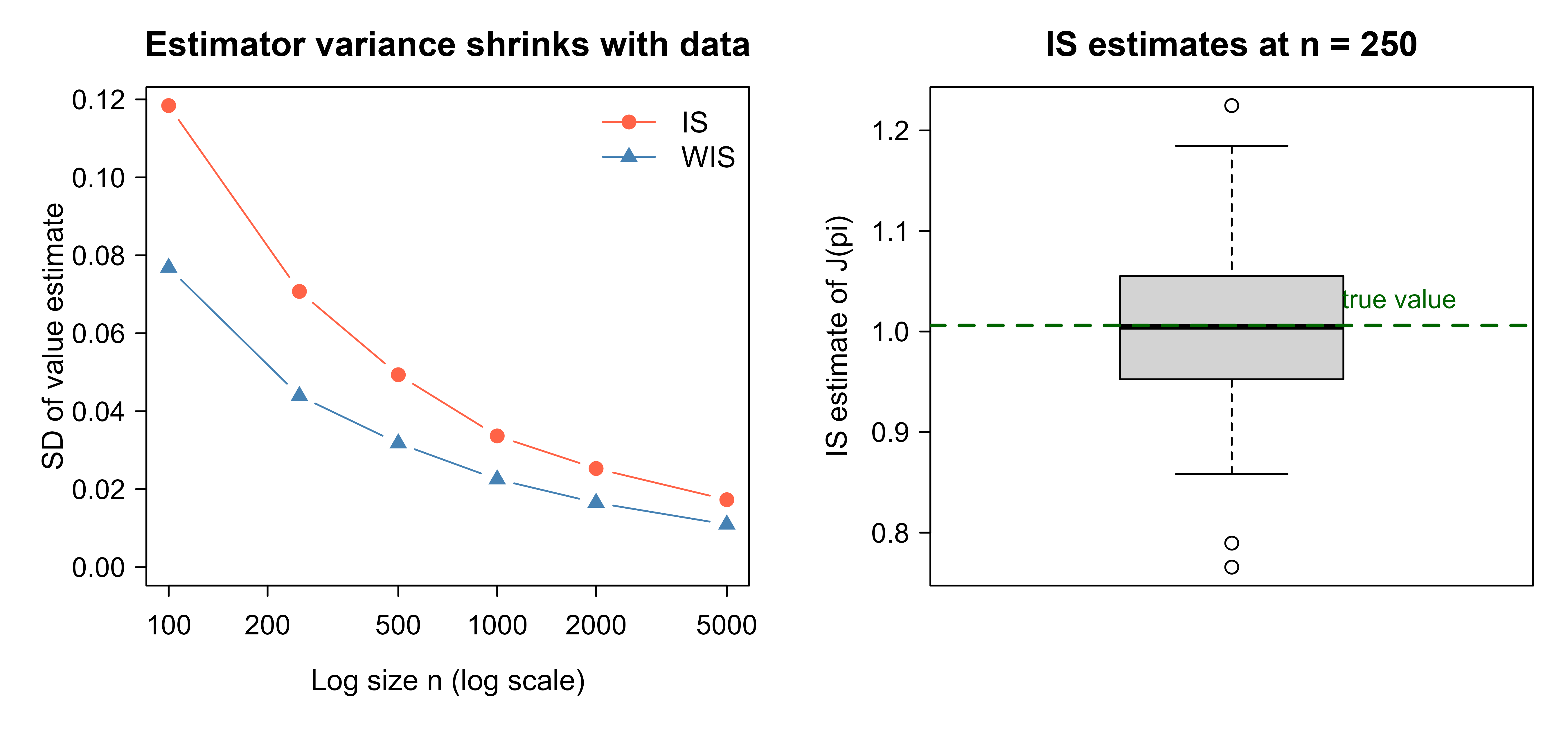
The table shows both estimators centering on the true value as \(n\) grows. Here the behavior and target policies overlap well, so the WIS finite-sample bias predicted by the theory is tiny and both means track the truth closely; the bias would become visible only with sharper policy divergence or smaller logs. Critically, the WIS standard deviation is smaller at every sample size, which is the variance reduction that makes WIS the safer default in practice. Figure 69.1 visualizes the same story: the spread of estimates around the true value shrinks with more data, and the WIS spread is tighter than the IS spread.
Show code
op<-par(mfrow =c(1, 2), mar =c(4.2, 4.2, 2.5, 1))# Left panel: standard deviation vs log size for IS and WIS.plot(conv$n, conv$IS_sd, type ="b", pch =19, col ="tomato", log ="x", xlab ="Log size n (log scale)", ylab ="SD of value estimate", main ="Estimator variance shrinks with data", ylim =range(0, conv$IS_sd, conv$WIS_sd))lines(conv$n, conv$WIS_sd, type ="b", pch =17, col ="steelblue")legend("topright", legend =c("IS", "WIS"), col =c("tomato", "steelblue"), pch =c(19, 17), lty =1, bty ="n")# Right panel: distribution of IS estimates at a single small sample size.set.seed(11)small_is<-replicate(200L, is_estimate(generate_log(250L)))boxplot(small_is, col ="lightgrey", ylab ="IS estimate of J(pi)", main ="IS estimates at n = 250", names ="")abline(h =J_true_target, lty =2, col ="darkgreen", lwd =2)text(x =1.3, y =J_true_target, labels ="true value", col ="darkgreen", pos =3, cex =0.9)par(op)
Figure 69.1: Off-policy evaluation accuracy versus log size. Left: standard deviation of the value estimate across 200 replications for ordinary IS and weighted IS, both shrinking as the log grows, with WIS consistently lower. Right: the distribution of individual IS estimates at n = 250 (boxplot) centered on the dashed true value, showing the estimator is unbiased but variable. Both panels form one figure.
The figure makes the bias-variance picture tangible. The left panel shows variance falling as the log grows and WIS dominating IS at every size; the right panel shows that at a small log size individual IS estimates scatter widely around the true value, even though they are centered on it. In a real offline RL pipeline, this is exactly the diagnostic you would run before trusting an OPE number: if the estimator’s variance at your actual log size is large relative to the differences between candidate policies, the evaluation cannot distinguish them and you need more data, lower-variance estimators, or a value model (the doubly robust route).
Tip
Read the demo as the OPE half of an offline RL system. A method like CQL would produce the candidate pi_target; the importance-sampling code here is how you would estimate its value from the same log before deployment, and how you would choose between candidates or settle CQL’s conservatism parameter. Learning the policy and evaluating it offline are two halves of one problem, and the evaluation half is where overconfidence is most easily caught.
69.8 Practical guidance and pitfalls
Offline RL projects fail in recognizable ways, and most failures trace back to ignoring the coverage of the dataset. The lessons that save the most time, roughly in the order you meet them:
Log the propensities. If you can influence data collection, record \(\pi_b(a \mid s)\) for the action actually taken. Importance sampling and doubly robust evaluation need these probabilities; reconstructing them after the fact from a deterministic or undocumented logging policy is error-prone and sometimes impossible.
Check coverage before anything else. Offline RL can only learn about state-action regions the data visited. If your target policy wants to act where \(\pi_b\) never went, no algorithm can rescue you, and importance weights become undefined. Plot the action distribution per state in your log and confirm the target policy stays within it.
Do not trust the training loss. A falling Bellman error or a high estimated value is not evidence of a good policy; naive methods report glowing numbers precisely when they are overestimating. The value the algorithm reports for itself is the least trustworthy number in the project.
Evaluate off-policy, and distrust high-variance estimates. Use WIS or doubly robust estimation, and report the variance of the estimate, not just its point value. If the variance swamps the gap between candidate policies, your evaluation cannot rank them.
Tune conservatism against OPE, not training loss. CQL’s \(\alpha\) and BCQ’s constraint width trade safety against improvement. The only honest way to set them is to evaluate the resulting policies off-policy on held-out logged data.
Prefer staying close to the data when stakes are high. In healthcare and other safety-critical settings, a policy that improves modestly but provably over \(\pi_b\) beats one that claims a large improvement built on extrapolation. Behavior-constrained methods make this conservatism explicit.
Know when offline RL is overkill. If the decisions are not sequential, a contextual bandit (Chapter 72) or supervised approach with off-policy evaluation may answer the question with far less machinery. Offline RL earns its complexity only when delayed, sequential effects are real.
Warning
The single most common and most dangerous mistake is treating a high self-reported value as success. Distributional shift makes naive offline RL optimistic by construction. Always confirm a policy’s value with a separate, low-variance off-policy estimator before believing it, and never deploy a policy whose advantage rests on regions of the state-action space your data never observed.
To summarize: offline RL learns a policy from a fixed log with no further interaction, which turns distributional shift into the central obstacle. Naive off-policy methods overestimate the value of unseen actions and exploit those errors, so the fixes either constrain the policy to the data’s support (BCQ and relatives) or learn deliberately pessimistic values (CQL). Off-policy evaluation, built on importance sampling and its lower-variance descendants, is how you judge a policy before deployment, and the base-R demo shows that reweighting logged rewards recovers a target policy’s true value while making the bias-variance trade-off concrete.
69.9 Further reading
Sutton and Barto (2018), Reinforcement Learning: An Introduction (2nd ed.). The standard reference; chapters on off-policy methods and importance sampling underpin this material.
Levine, Kumar, Tucker, and Fu (2020), Offline Reinforcement Learning: Tutorial, Review, and Perspectives on Open Problems. A thorough survey of the field and its central challenges.
Fujimoto, Meger, and Precup (2019), Off-Policy Deep Reinforcement Learning without Exploration. Introduces BCQ and diagnoses extrapolation error.
Kumar, Zhou, Tucker, and Levine (2020), Conservative Q-Learning for Offline Reinforcement Learning. The CQL algorithm.
Kumar, Fu, Tucker, and Levine (2019), Stabilizing Off-Policy Q-Learning via Bootstrapping Error Reduction. Introduces BEAR.
Fujimoto and Gu (2021), A Minimalist Approach to Offline Reinforcement Learning. Introduces TD3+BC.
Jiang and Li (2016), Doubly Robust Off-policy Value Evaluation for Reinforcement Learning. The doubly robust OPE estimator for sequential problems.
Dudík, Langford, and Li (2011), Doubly Robust Policy Evaluation and Learning. Doubly robust estimation in the contextual-bandit setting.
Precup, Sutton, and Singh (2000), Eligibility Traces for Off-Policy Policy Evaluation. Foundational work on importance-sampling-based OPE.
Source Code
# Offline (Batch) Reinforcement Learning {#sec-offline-rl}```{r}#| include: falsesource("_common.R")```Picture a hospital with ten years of records: for each patient visit, the clinician's chosen treatment, the patient's state before and after, and the eventual outcome. You would like to learn a better treatment policy. You cannot run the obvious reinforcement learning experiment, which would mean letting an agent try treatments on real patients and learn from the results, because experimenting on people is unethical and slow. All you have is the log. Offline reinforcement learning (also called batch RL) is reinforcement learning under exactly this constraint: learn the best policy you can from a fixed dataset of past interactions, with no ability to gather new data by acting.This is a different problem from the one in the deep reinforcement learning chapter (@sec-deep-reinforcement-learning), where the agent could always try an action and observe what happened. That freedom is what online RL relies on, and it is precisely what offline RL gives up. The dataset was generated by some behavior policy $\pi_b$ (the clinicians, the old recommender, the human operators), and that is the only window onto the environment you will ever get. The question is no longer "how should the agent explore?" but "given this frozen record of someone else's decisions, what is the best policy I can justify, and how do I avoid fooling myself?"::: {.callout-tip title="Intuition"}Online RL is learning to cook by tasting as you go. Offline RL is learning to cook from a stack of other people's recipes and reviews, with the kitchen locked. You can reason about combinations nobody wrote down, but you can never taste them, so you have to be honest about how far you are extrapolating beyond what the recipes actually tried.:::This chapter explains why the obvious approach (run a standard off-policy algorithm on the logged data) fails, sometimes catastrophically, and what to do instead. We build intuition for the central pathology, distributional shift and its companion extrapolation error, then formalize it. We cover the two dominant families of fixes: constrain the learned policy to stay near the behavior policy (BCQ), and learn value estimates that are deliberately pessimistic about unseen actions (CQL). We then turn to a question that matters as much as learning the policy: how do you estimate how good a policy is, using only logged data, before you ever deploy it? That is off-policy evaluation (OPE), and importance sampling is its workhorse. The runnable demo at the end implements importance sampling OPE in base R on a small simulated logged dataset and checks the estimate against ground truth, which we can compute precisely because the simulation's true dynamics are known.::: {.callout-tip title="When to use this"}Reach for offline RL when interaction is expensive, dangerous, or impossible, but logs of past decisions are plentiful: clinical treatment from electronic health records, recommendation and ad systems with click logs, robotics from teleoperation or prior runs, industrial control from historical operation. If you can interact cheaply and safely, online RL is simpler and usually better. If decisions are not sequential, an offline bandit or supervised approach may be enough.:::## Setup and notationWe work in the same Markov decision process (MDP) $(\mathcal{S}, \mathcal{A}, P, R, \gamma)$ used in the deep RL chapter (@sec-deep-reinforcement-learning): $\mathcal{S}$ is the state space, $\mathcal{A}$ the action space, $P(s' \mid s, a)$ the transition kernel, $R(s, a)$ the expected immediate reward, and $\gamma \in [0, 1)$ the discount factor. A policy $\pi(a \mid s)$ is a distribution over actions given a state, and the object we care about is the expected discounted return, or value, of a policy,$$J(\pi) = \mathbb{E}_{\pi}\!\left[ \sum_{t=0}^{\infty} \gamma^t\, r_t \right],$$where the expectation is over trajectories generated by following $\pi$ in the environment.It will be convenient to have the standard value-function machinery in place, since every offline algorithm manipulates it. Define the state-action value (Q-function) and state value of a policy $\pi$ as$$Q^\pi(s,a) = \mathbb{E}_\pi\!\left[\sum_{t=0}^\infty \gamma^t r_t \,\Big|\, s_0 = s, a_0 = a\right],\qquadV^\pi(s) = \mathbb{E}_{a\sim\pi(\cdot\mid s)}[Q^\pi(s,a)] .$$These satisfy the Bellman expectation equation $Q^\pi(s,a) = R(s,a) + \gamma \,\mathbb{E}_{s'\sim P(\cdot\mid s,a)}\,V^\pi(s')$, and the optimal value $Q^\star$ satisfies the Bellman optimality equation $Q^\star(s,a) = R(s,a) + \gamma\,\mathbb{E}_{s'}\,\max_{a'}Q^\star(s',a')$. If $d_0$ is the initial-state distribution then $J(\pi) = \mathbb{E}_{s\sim d_0}[V^\pi(s)]$. We write the Bellman optimality operator as $(\mathcal{T}Q)(s,a) = R(s,a) + \gamma\,\mathbb{E}_{s'}\,\max_{a'}Q(s',a')$, and the policy-evaluation operator as $(\mathcal{T}^\pi Q)(s,a) = R(s,a) + \gamma\,\mathbb{E}_{s'}\,\mathbb{E}_{a'\sim\pi}\,Q(s',a')$.::: {.callout-note title="Why these operators are the whole game"}Both $\mathcal{T}$ and $\mathcal{T}^\pi$ are $\gamma$-contractions in the sup norm: for any $Q_1, Q_2$,$$\|\mathcal{T}Q_1 - \mathcal{T}Q_2\|_\infty \le \gamma\,\|Q_1 - Q_2\|_\infty .$$The proof is one line. For fixed $(s,a)$, $|(\mathcal{T}Q_1 - \mathcal{T}Q_2)(s,a)| = \gamma\,|\mathbb{E}_{s'}(\max_{a'}Q_1(s',a') - \max_{a'}Q_2(s',a'))| \le \gamma\,\mathbb{E}_{s'}\max_{a'}|Q_1(s',a') - Q_2(s',a')| \le \gamma\,\|Q_1 - Q_2\|_\infty$, using $|\max_x f - \max_x g| \le \max_x|f-g|$. By Banach's fixed-point theorem the iteration $Q_{k+1} = \mathcal{T}Q_k$ converges geometrically to the unique fixed point $Q^\star$ at rate $\gamma$. Offline RL does not change this fixed-point logic; it changes the fact that the expectation $\mathbb{E}_{s'}$ inside the operator must be estimated from a fixed sample, and that the $\max_{a'}$ can land on actions the sample never covers. That is exactly where the trouble in @sec-offline-rl enters.:::What makes the problem offline is the data. We are handed a fixed dataset$$\mathcal{D} = \{ (s_i, a_i, r_i, s_i') \}_{i=1}^{n},$$a collection of transitions logged while some behavior policy $\pi_b$ was in control. We never get to choose $s_i$ or $a_i$; they are whatever the log contains. The goal is to produce a target policy $\pi$ (sometimes written $\pi_e$ for "evaluation" or "target") with high $J(\pi)$, and ideally to estimate $J(\pi)$ from $\mathcal{D}$ alone before deploying it. We write $\hat{J}(\pi)$ for such an estimate.::: {.callout-note}Offline RL is "off-policy" in the technical sense (the data comes from $\pi_b$, not the policy we want to evaluate or improve), but it adds a hard extra constraint: there is no more data, ever. Many off-policy algorithms that work fine online, where they can interleave a little fresh exploration, break when that lifeline is removed. The next section explains why.:::## Why naive off-policy methods failThe tempting move is to take an off-policy algorithm that already works online, such as Q-learning or its deep cousin DQN, point it at the logged dataset, and run gradient steps until the value estimates converge. This usually produces a policy that looks excellent on paper and behaves terribly in deployment. Three intertwined effects explain the failure.### Distributional shiftA learned policy $\pi$ is useful only if it differs from the behavior policy $\pi_b$, otherwise you have just copied the past. But the moment $\pi$ chooses actions $\pi_b$ rarely or never took, it steers the system into states the dataset barely covers. The distribution of states and actions the learned policy visits, call it $d^{\pi}$, drifts away from the distribution the data was drawn from, $d^{\pi_b}$. This mismatch is distributional shift, and it is the root cause from which the other two problems grow.::: {.callout-tip title="Intuition"}Your dataset is a map of the territory the behavior policy walked. The learned policy wants to take a shortcut through a region the map never surveyed. The value estimates for that region are not measurements; they are guesses extrapolated from elsewhere, and the optimizer will happily march straight into them.:::### Extrapolation errorA value function trained on $\mathcal{D}$ is only constrained where $\mathcal{D}$ has data. For a state-action pair $(s, a)$ that never appears, $Q(s, a)$ is whatever the function approximator extrapolates, and that value is unconstrained by any observation. With a table, unseen entries keep their initial value; with a neural network, they take whatever the network's smoothness happens to produce. Either way, the estimate carries no information about the true return. This is extrapolation error: confident-looking values for actions the data cannot speak to.### Overestimation and the bootstrapping trapThe two effects above would be merely inconvenient if the algorithm treated unknown values as unknown. The disaster is that Q-learning's update actively seeks them out. Recall the bootstrapped target$$Q(s, a) \leftarrow r + \gamma \max_{a'} Q(s', a').$$The $\max$ over next actions $a'$ deliberately selects the highest value at $s'$. If any out-of-distribution action has an erroneously high estimate (and extrapolation guarantees some will), the $\max$ picks it, and that inflated value propagates backward into other states through bootstrapping. The errors do not average out; they are systematically selected and amplified. Online, the agent would try the over-valued action, observe a disappointing reward, and correct the estimate. Offline, that correction never comes, because the agent cannot act. The values climb without bound and the resulting greedy policy chases a mirage.::: {.callout-warning}This is the defining failure of offline RL. Standard off-policy algorithms run on static data tend to overestimate the value of out-of-distribution actions, then exploit those overestimates, producing policies far worse than the behavior policy that generated the data (Fujimoto et al., 2019; Levine et al., 2020). More gradient steps make it worse, not better. Every method in the next section is, at heart, a way to stop the algorithm from trusting values it has no right to trust.:::### Why the bias is upward, made preciseIt is worth seeing that the overestimation is not bad luck but a systematic upward bias built into the $\max$ operator, the same mechanism that motivates Double Q-learning online. Suppose at state $s'$ the true values $Q^\star(s',a')$ are estimated with independent zero-mean errors, $\hat Q(s',a') = Q^\star(s',a') + \varepsilon_{a'}$ with $\mathbb{E}[\varepsilon_{a'}] = 0$. Even though each estimate is unbiased, the bootstrapped target uses $\max_{a'}\hat Q(s',a')$, and by Jensen's inequality applied to the convex $\max$ function,$$\mathbb{E}\Big[\max_{a'}\hat Q(s',a')\Big] \;\ge\; \max_{a'}\,\mathbb{E}\big[\hat Q(s',a')\big] \;=\; \max_{a'}Q^\star(s',a') .$$The gap is strictly positive whenever the errors are non-degenerate, and it grows with both the noise scale and the number of candidate actions $|\mathcal{A}|$. For independent Gaussian errors $\varepsilon_{a'}\sim\mathcal{N}(0,\sigma^2)$ with $m=|\mathcal{A}|$ tied true values, the bias is the expected maximum of $m$ standard normals, $\sigma\,\mathbb{E}[\max_j Z_j] \approx \sigma\sqrt{2\ln m}$, which increases without bound in $m$. Online, the agent samples the over-valued action, the realized return contradicts $\varepsilon_{a'}$, and the estimate is pulled back. Offline, the value $Q^\star(s',a')$ for an out-of-distribution $a'$ is never measured, so $\varepsilon_{a'}$ is whatever the function approximator extrapolates and is never corrected; the positive bias is then injected into the target and, because $\mathcal{T}$ propagates it through bootstrapping, accumulates across the horizon as a geometric series with ratio $\gamma$, reaching up to $\tfrac{1}{1-\gamma}$ times the per-step bias. This is the formal content of "errors are selected and amplified."## Behavior-constrained methods: BCQThe first family of fixes attacks distributional shift directly: forbid the learned policy from taking actions the behavior policy would not plausibly take. If $\pi$ only ever proposes actions that lie in the support of $\pi_b$, then the $\max$ in the Bellman target never reaches an out-of-distribution action, and the overestimation loop is broken at its source.Batch-Constrained deep Q-learning (BCQ; Fujimoto et al., 2019) is the canonical instance. Its insight is to restrict the maximization in the Bellman update to actions the data supports. Conceptually, BCQ learns a generative model $\hat{\pi}_b(a \mid s)$ of the behavior policy, samples candidate actions from it, optionally perturbs them slightly, and takes the $\max$ over only those candidates rather than over the entire action space:$$Q(s, a) \leftarrow r + \gamma \max_{a' \,\in\, \text{support}(\hat{\pi}_b(\cdot \mid s'))} Q(s', a').$$The constraint is a tunable knob. A tight constraint keeps $\pi$ close to $\pi_b$ (safe, but it cannot improve much beyond imitation); a loose constraint allows more deviation (more potential gain, more extrapolation risk). In the limit of an infinitely tight constraint, BCQ reduces to behavior cloning, simply imitating $\pi_b$.::: {.callout-important title="Key idea"}Behavior-constrained methods change the question from "what is the best action anywhere?" to "what is the best action among those the data can vouch for?" The optimizer is no longer allowed to wander off the map. This is a support constraint, not a distribution-matching constraint: $\pi$ may weight the supported actions very differently from $\pi_b$, it just may not invent new ones.:::Related methods enforce the closeness differently. BEAR (Kumar et al., 2019) constrains the maximum mean discrepancy between $\pi$ and $\pi_b$; TD3+BC (Fujimoto and Gu, 2021) simply adds a behavior-cloning penalty to a standard actor-critic loss, a strikingly simple recipe that is competitive in practice. All share the philosophy: stay near the data.### The constrained objective and the error bound it controlsThe various behavior-constrained methods are instances of one constrained optimization. Write the policy improvement step as$$\pi^{\text{new}} = \arg\max_{\pi}\; \mathbb{E}_{s\sim\mathcal{D}}\,\mathbb{E}_{a\sim\pi(\cdot\mid s)}\big[\hat Q(s,a)\big]\quad\text{subject to}\quad\mathbb{E}_{s\sim\mathcal{D}}\,D\!\big(\pi(\cdot\mid s)\,\big\|\,\hat\pi_b(\cdot\mid s)\big) \le \epsilon ,$$ {#eq-offline-rl-bcq-constrained}where $D$ is a divergence (a hard support constraint for BCQ, MMD for BEAR, KL for the penalized variants) and $\epsilon$ is the constraint budget. TD3+BC is the Lagrangian relaxation with $D$ the squared action distance and a fixed multiplier, giving the loss $\mathbb{E}[-\lambda \hat Q(s,\pi(s)) + (\pi(s) - a)^2]$. The reason a small $\epsilon$ is principled, and not merely cautious, is a performance-difference bound. By the standard simulation lemma, for any two policies,$$J(\pi) - J(\pi_b) = \frac{1}{1-\gamma}\,\mathbb{E}_{s\sim d^{\pi}}\,\mathbb{E}_{a\sim\pi(\cdot\mid s)}\big[A^{\pi_b}(s,a)\big],$$where $A^{\pi_b} = Q^{\pi_b} - V^{\pi_b}$ is the advantage under the behavior policy and $d^{\pi}$ is the (discounted) state-visitation distribution of $\pi$. The catch is that $d^{\pi}$ is unknown offline. Replacing it with $d^{\pi_b}$ introduces an error controlled by the total-variation distance between the visitation distributions, which itself is bounded (via the coupling argument behind the bound of Schulman et al. on monotonic improvement) by $\tfrac{2\gamma}{(1-\gamma)^2}\,\max_s D_{\mathrm{TV}}(\pi(\cdot\mid s)\,\|\,\pi_b(\cdot\mid s))$. Keeping $D \le \epsilon$ keeps this surrogate gap small, so the empirical improvement computed on $d^{\pi_b}$ is a trustworthy proxy for the true improvement. This is the rigorous reason the constraint width trades safety (small $\epsilon$, tight bound, little extrapolation) against potential gain (large $\epsilon$, loose bound).## Conservative value estimation: CQLThe second family attacks the symptom rather than the action set: if the trouble is overestimated values for unseen actions, then learn values that are deliberately pessimistic there. Make the algorithm assume the worst about actions it has not seen, so it has no incentive to choose them.Conservative Q-Learning (CQL; Kumar et al., 2020) adds a regularizer to the standard Bellman objective that pushes down the $Q$ values of actions sampled from the current policy while pushing up the $Q$ values of actions actually present in the data. Schematically, the objective augments the usual TD error with$$\min_{Q}\; \alpha \left( \mathbb{E}_{s \sim \mathcal{D},\, a \sim \pi}[Q(s, a)] - \mathbb{E}_{(s,a) \sim \mathcal{D}}[Q(s, a)] \right) + \tfrac{1}{2}\, \mathbb{E}_{\mathcal{D}}\big[(Q - \mathcal{B}Q)^2\big],$$where $\mathcal{B}Q$ is the Bellman target and $\alpha > 0$ controls the strength of the conservatism. The first term lowers values for whatever the policy wants to do (which includes out-of-distribution actions) and raises values for what the data did, so the gap that the optimizer would exploit closes. The result is a $Q$ function that lower-bounds the true value of the learned policy, a lower bound rather than an unbiased estimate, on purpose.### Deriving the conservative lower boundThe claim that CQL produces a lower bound is not asserted; it falls out of a one-step minimization. Consider, at a fixed state $s$ with empirical behavior distribution $\hat\pi_b(\cdot\mid s)$, the simplest conservative objective that penalizes a policy distribution $\mu(\cdot\mid s)$ and rewards the data distribution, subject to the usual Bellman regression. Drop the regression term for a moment and minimize over the function value $\hat Q(s,a)$ the penalty$$\min_{\hat Q}\;\; \alpha\Big(\mathbb{E}_{a\sim\mu}[\hat Q(s,a)] - \mathbb{E}_{a\sim\hat\pi_b}[\hat Q(s,a)]\Big) + \tfrac{1}{2}\,\mathbb{E}_{a\sim\hat\pi_b}\big[(\hat Q(s,a) - (\mathcal{B}^\pi \hat Q)(s,a))^2\big].$$Setting the derivative with respect to $\hat Q(s,a)$ to zero (the empirical state-action distribution puts mass $\hat\pi_b(a\mid s)$ on each $a$) gives, for actions in the support of the data,$$\hat Q(s,a) = (\mathcal{B}^\pi \hat Q)(s,a) - \alpha\,\frac{\mu(a\mid s) - \hat\pi_b(a\mid s)}{\hat\pi_b(a\mid s)} .$$ {#eq-offline-rl-cql-fixedpoint}The correction subtracted from the Bellman backup is exactly $\alpha$ times the importance ratio $\mu/\hat\pi_b$ minus one. Wherever the evaluated policy $\mu$ places more mass than the data did, $\mu(a\mid s) > \hat\pi_b(a\mid s)$, the correction is positive and the value is pushed strictly below the Bellman target; where the policy matches the data the correction vanishes. Taking the expectation under $\mu$ to form the value estimate,$$\hat V^\mu(s) = \mathbb{E}_{a\sim\mu}[\hat Q(s,a)] = \mathbb{E}_{a\sim\mu}[(\mathcal{B}^\pi\hat Q)(s,a)] - \alpha\,\underbrace{\sum_a \frac{(\mu(a\mid s) - \hat\pi_b(a\mid s))^2}{\hat\pi_b(a\mid s)}}_{\ge\,0,\ =\,\chi^2(\mu\,\|\,\hat\pi_b)} .$$The subtracted quantity is a chi-square divergence between the evaluated policy and the behavior policy, which is non-negative and is zero only when $\mu = \hat\pi_b$. Hence for any $\alpha > 0$ the estimated value lower-bounds the true value of the policy, $\hat V^\mu(s) \le V^\mu(s)$, with a slack that grows with how far the policy strays from the data. This is the precise sense in which CQL is conservative: the penalty is a divergence, the bound is one-sided, and $\alpha$ scales the gap. A refinement of the analysis (Kumar et al., 2020) shows that with sampling error of order $C_{s,a}/\sqrt{n_{s,a}}$ in the Bellman backup, choosing $\alpha$ large enough to dominate that error preserves the lower bound with high probability, which is the theoretical reason $\alpha$ should be larger when per-state counts $n_{s,a}$ are small.::: {.callout-tip title="Intuition"}BCQ fences off the unseen actions so the optimizer cannot reach them. CQL leaves the fence open but salts the ground outside it, so nothing the optimizer finds out there looks appealing. Both arrive at the same destination, a policy that prefers what the data supports, by different routes. CQL needs no separate generative model of $\pi_b$, which makes it a popular default.:::::: {.callout-warning}Conservatism is a dial, not a free lunch. Set $\alpha$ too low and overestimation creeps back; set it too high and the policy becomes so pessimistic it refuses any improvement over the behavior policy. The right setting depends on how much of the state-action space the data covers, and it cannot be tuned by training loss alone. This is where off-policy evaluation, below, becomes indispensable.:::Because BCQ and CQL rely on neural function approximation and a gradient-based training loop, a complete implementation belongs with the deep learning tooling rather than base R. The sketch below shows the shape of a CQL loss in `torch` for R; it is kept `eval=FALSE` because it is a reference, not a runnable demo, and it omits the surrounding training loop and replay machinery.```{r offline-rl-cql-sketch, eval=FALSE}library(torch)# Conservative Q-Learning loss for discrete actions.# q_net(states) returns a tensor of shape [batch, n_actions].cql_loss <-function(q_net, target_q_net, batch, gamma =0.99, alpha =1.0) { q_all <-q_net(batch$states) # [B, A] q_taken <- q_all$gather(2, batch$actions$unsqueeze(2))$squeeze(2)# Standard TD target using the target network.with_no_grad({ q_next <-target_q_net(batch$next_states) # [B, A] max_next <- q_next$max(dim =2)[[1]] td_target <- batch$rewards + gamma * max_next * (1- batch$done) }) bellman_error <-nnf_mse_loss(q_taken, td_target)# Conservative term: logsumexp over all actions (what the policy could# pick, including unseen ones) minus the value of the logged action. logsumexp_q <-torch_logsumexp(q_all, dim =2) # pushes down OOD actions conservative <- (logsumexp_q - q_taken)$mean() # pushes up data actions bellman_error + alpha * conservative}```## Off-policy evaluationSuppose someone hands you a candidate policy $\pi$. Before you deploy it on patients or live traffic, you want to know $J(\pi)$, its expected return, using only the logged data $\mathcal{D}$ collected under $\pi_b$. This is off-policy evaluation (OPE). It is the offline counterpart of a held-out test set, and it is what lets you compare policies and tune hyperparameters (such as CQL's $\alpha$) without touching the real system.### Importance samplingThe foundational OPE estimator is importance sampling (IS), the same reweighting trick used throughout Monte Carlo statistics. The idea: we have samples drawn under $\pi_b$ but want an expectation under $\pi$, so we reweight each sample by how much more (or less) likely $\pi$ was to produce it than $\pi_b$ was.For a single decision (the contextual-bandit, one-step case; see @sec-contextual-bandits), let the logged dataset contain tuples $(s_i, a_i, r_i)$ where action $a_i$ was drawn from $\pi_b(\cdot \mid s_i)$ and earned reward $r_i$. The IS estimate of the target policy's value is$$\hat{J}_{\text{IS}}(\pi) = \frac{1}{n} \sum_{i=1}^{n} \rho_i\, r_i,\qquad\rho_i = \frac{\pi(a_i \mid s_i)}{\pi_b(a_i \mid s_i)},$$where $\rho_i$ is the importance weight. The algebra that makes this work is short:$$\mathbb{E}_{a \sim \pi_b}\!\left[ \frac{\pi(a \mid s)}{\pi_b(a \mid s)}\, r(s, a) \right]= \sum_{a} \pi_b(a \mid s)\, \frac{\pi(a \mid s)}{\pi_b(a \mid s)}\, r(s, a)= \sum_{a} \pi(a \mid s)\, r(s, a)= \mathbb{E}_{a \sim \pi}[r(s, a)].$$The $\pi_b$ in the numerator and denominator cancel, leaving an expectation under $\pi$. So $\hat{J}_{\text{IS}}$ is unbiased: on average it returns the true value of $\pi$, even though every sample was collected under a different policy.::: {.callout-important title="Key idea"}Importance sampling lets you ask "what would the average reward have been if the target policy had been in control?" using data the behavior policy generated. Actions the target policy favors get up-weighted; actions it would have avoided get down-weighted toward zero. The behavior probabilities must be known (or estimated), which is why logging the propensities $\pi_b(a \mid s)$ at collection time is a best practice worth insisting on.:::For full multi-step trajectories, the per-step weights multiply along the trajectory, and the estimator weights the whole-trajectory return by the cumulative product$$\rho_{0:T} = \prod_{t=0}^{T} \frac{\pi(a_t \mid s_t)}{\pi_b(a_t \mid s_t)}.$$This product is the source of IS's central weakness: variance. If a trajectory is even modestly long, or if $\pi$ and $\pi_b$ differ much per step, the product can explode toward huge values for a few trajectories and collapse to near zero for the rest, so the estimate ends up dominated by a handful of samples.::: {.callout-warning}Importance sampling is unbiased but its variance grows, often exponentially, with horizon length and with the divergence between $\pi$ and $\pi_b$. An unbiased estimator with enormous variance is not useful in practice. The next subsection covers the standard variance-reduction fixes.:::### The variance of importance sampling, quantifiedThe qualitative warning becomes precise once we compute the variance. In the one-step case, the per-sample IS estimator $\rho_i r_i$ is i.i.d., so $\operatorname{Var}(\hat J_{\text{IS}}) = \tfrac{1}{n}\operatorname{Var}(\rho\,r)$. Writing $\rho = \pi(a\mid s)/\pi_b(a\mid s)$ and using $\mathbb{E}_{\pi_b}[\rho\,r] = J(\pi)$,$$\operatorname{Var}(\rho\, r) = \mathbb{E}_{\pi_b}[\rho^2 r^2] - J(\pi)^2 .$$The second moment of the weight alone is the key driver. With $r$ bounded by $R_{\max}$,$$\mathbb{E}_{\pi_b}[\rho^2] = \sum_a \pi_b(a\mid s)\left(\frac{\pi(a\mid s)}{\pi_b(a\mid s)}\right)^2 = \sum_a \frac{\pi(a\mid s)^2}{\pi_b(a\mid s)} = 1 + \chi^2\!\big(\pi(\cdot\mid s)\,\|\,\pi_b(\cdot\mid s)\big),$$so the variance is governed by the same chi-square divergence that appeared in the CQL bound: the more $\pi$ concentrates where $\pi_b$ was reluctant, the heavier the weights. This is the formal statement that variance grows with policy divergence, and it shows that overlap is not optional: if $\pi_b(a\mid s)\to 0$ while $\pi(a\mid s) > 0$, the chi-square term, and hence the variance, diverges.For the $T$-step trajectory estimator the weights multiply, and under the (worst-case) assumption that per-step ratios are independent with second moment $1 + \chi^2$ at each step, the trajectory weight has second moment $(1+\chi^2)^{T+1}$. The variance therefore scales as$$\operatorname{Var}(\hat J_{\text{IS}}) = O\!\left(\frac{(1+\chi^2)^{T}}{n}\right),$$exponential in the horizon. This is the "curse of horizon" for trajectory IS and the reason per-step (per-decision) importance sampling, which only multiplies the weights up to the time of each reward rather than over the whole trajectory, is preferred: it removes the dependence of early rewards on later, irrelevant ratios and strictly reduces variance without adding bias.::: {.callout-note title="Effective sample size diagnostic"}The practical proxy for "how many of my $n$ samples actually count" is the effective sample size $\mathrm{ESS} = (\sum_i \rho_i)^2 / \sum_i \rho_i^2$, which ranges from $1$ (one weight dominates) to $n$ (all weights equal). When $\mathrm{ESS} \ll n$ the IS estimate rests on a handful of trajectories and should not be trusted; this is the single most useful number to report alongside any IS-based OPE value.:::### Variance reduction: weighted IS and doubly robust estimationTwo refinements tame the variance. Weighted importance sampling (WIS, also called self-normalized IS) normalizes by the sum of weights rather than by $n$:$$\hat{J}_{\text{WIS}}(\pi) = \frac{\sum_{i=1}^{n} \rho_i\, r_i}{\sum_{i=1}^{n} \rho_i}.$$WIS is biased (the bias vanishes as $n \to \infty$) but typically has far lower variance, because the normalization keeps a few large weights from blowing up the estimate. In practice WIS is almost always more reliable than ordinary IS, and the bias-variance trade it makes is usually worth it.The doubly robust (DR) estimator (Jiang and Li, 2016; Dudík et al., 2011) combines IS with a learned model $\hat{Q}$ of the value function. It uses the model as a baseline and applies the importance weight only to the residual reward the model failed to predict:$$\hat{J}_{\text{DR}}(\pi) = \frac{1}{n}\sum_{i=1}^{n}\Big[ \hat{V}(s_i) + \rho_i\big( r_i - \hat{Q}(s_i, a_i) \big) \Big],\qquad \hat{V}(s) = \sum_{a}\pi(a \mid s)\,\hat{Q}(s, a).$$It is "doubly robust" because it is consistent if either the importance weights are correct or the value model $\hat{Q}$ is correct; you get two chances to be right. When the model is good, the residual is small, the weighted term contributes little variance, and the estimate is both low-variance and unbiased. @tbl-offline-rl-ope-comparison compares the three estimators on the properties that matter when choosing one.### Why DR is doubly robust, and why WIS is biasedThe double-robustness property follows from a short bias calculation. Take expectations of the one-step DR term under the behavior policy and decompose around the truth. Let the true per-action mean be $Q(s,a) = \mathbb{E}[r\mid s,a]$ and $V(s) = \mathbb{E}_{a\sim\pi}[Q(s,a)]$. The bias of the DR estimator is$$\mathbb{E}_{\pi_b}\big[\hat V(s) + \rho\,(r - \hat Q(s,a))\big] - V(s)= \big(\hat V(s) - V(s)\big) + \mathbb{E}_{\pi_b}\big[\rho\,(r - \hat Q(s,a))\big] .$$Now $\mathbb{E}_{\pi_b}[\rho\,(r - \hat Q(s,a))] = \mathbb{E}_{a\sim\pi}[Q(s,a) - \hat Q(s,a)]$ because the importance weight converts the $\pi_b$ expectation to a $\pi$ expectation and $\mathbb{E}[r\mid s,a] = Q(s,a)$. Adding $\hat V(s) - V(s) = \mathbb{E}_{a\sim\pi}[\hat Q(s,a) - Q(s,a)]$, the two terms cancel exactly:$$\text{bias} = \mathbb{E}_{a\sim\pi}[\hat Q(s,a) - Q(s,a)] + \mathbb{E}_{a\sim\pi}[Q(s,a) - \hat Q(s,a)] = 0 .$$This used the correct weights. If instead the model is exact ($\hat Q = Q$) but the weights are wrong, $\hat\rho \ne \rho$, then $r - \hat Q$ has conditional mean zero, so $\mathbb{E}[\hat\rho\,(r - \hat Q)\mid s,a] = 0$ regardless of $\hat\rho$, and again only the $\hat V(s) = V(s)$ term survives, giving zero bias. Either ingredient being correct suffices; that is the "double" in doubly robust. The residual $r - \hat Q$ also explains the variance reduction: the importance weight multiplies only the part of the reward the model fails to predict, so a good model shrinks the high-variance weighted term toward zero. With a consistent model the high-variance weighted term reduces to $\mathbb{E}_{\pi_b}[\rho^2\operatorname{Var}(r\mid s,a)]/n$, replacing the full second moment $\mathbb{E}_{\pi_b}[\rho^2 r^2]$ of plain IS; the total per-sample DR variance is $\operatorname{Var}(\hat J_{\text{DR}}) = \big[\operatorname{Var}_{s}(\hat V(s)) + \mathbb{E}_{\pi_b}[\rho^2\operatorname{Var}(r\mid s,a)]\big]/n$, the extra term being the variance of the baseline $\hat V(s)$ across states.The bias of WIS comes from its denominator. The self-normalized estimator $\hat J_{\text{WIS}} = \sum_i \rho_i r_i / \sum_i \rho_i$ is a ratio of two random sums. Even though $\mathbb{E}[\tfrac{1}{n}\sum_i \rho_i] = 1$ and $\mathbb{E}[\tfrac{1}{n}\sum_i \rho_i r_i] = J(\pi)$ individually, the expectation of the ratio is not the ratio of expectations: by the standard delta-method expansion for $\mathbb{E}[X/Y]$ around $(\mu_X,\mu_Y) = (J,1)$,$$\mathbb{E}[\hat J_{\text{WIS}}] \approx J(\pi) - \frac{\operatorname{Cov}(\tfrac1n\sum\rho_i r_i,\ \tfrac1n\sum\rho_i)}{\mu_Y} + J(\pi)\,\operatorname{Var}\!\big(\tfrac1n\textstyle\sum\rho_i\big) = J(\pi) + O(1/n) .$$The bias is $O(1/n)$ and therefore vanishes as $n\to\infty$ (WIS is consistent), but it is the price paid for the variance reduction that the normalization buys, since dividing by $\sum_i\rho_i$ rather than $n$ cancels much of the fluctuation in the weights themselves.```{r tbl-offline-rl-ope-comparison, echo=FALSE}ope_tbl <-data.frame(Estimator =c("Importance sampling (IS)","Weighted IS (WIS)","Doubly robust (DR)"),Bias =c("Unbiased","Biased, vanishes as n grows","Unbiased if weights or model correct"),Variance =c("High; grows with horizon","Lower; normalization caps weights","Low when value model is accurate"),Needs =c("Behavior propensities pi_b","Behavior propensities pi_b","Propensities plus a value model Q-hat"),stringsAsFactors =FALSE)knitr::kable( ope_tbl,caption ="Off-policy evaluation estimators compared on bias, variance, and what each requires as input. Weighted IS trades a little bias for much lower variance; doubly robust adds a value model to cut variance further while staying unbiased if either component is correct.",col.names =c("Estimator", "Bias", "Variance", "Requires"),align =c("l", "l", "l", "l"))```::: {.callout-note}Importance sampling of any flavor requires overlap (also called coverage): wherever $\pi$ puts probability on an action, $\pi_b$ must have put nonzero probability too, so $\pi_b(a \mid s) > 0$ whenever $\pi(a \mid s) > 0$. If the target policy can take an action the behavior policy never tried, the weight is undefined (a division by zero) and no amount of cleverness recovers the missing information. This is the OPE face of the same coverage requirement that governs whether offline RL is feasible at all.:::## Coverage, concentrability, and what is information-theoretically possibleBoth the policy-learning and the evaluation halves of offline RL are limited by the same quantity: how well the data distribution covers the states and actions the target policy visits. This can be made into a single scalar, the concentrability coefficient,$$C^\pi = \max_{s,a}\,\frac{d^\pi(s,a)}{d^{\pi_b}(s,a)},$$the largest ratio of the discounted visitation density of the target policy to that of the behavior policy. When $C^\pi$ is finite, the data covers everything $\pi$ does (every state-action $\pi$ reaches was reached by $\pi_b$ with comparable frequency); when it is infinite, $\pi$ visits something the data never saw, and no estimator can recover the missing return. Error bounds for approximate dynamic programming on offline data take the form$$\|Q^\star - Q^{\pi_k}\|_{1,d_0} \;\le\; \frac{2\gamma}{(1-\gamma)^2}\,C^\pi\,\max_k \|\,Q_k - \mathcal{T}Q_k\,\|_{2,d^{\pi_b}} ,$$which says the suboptimality of the learned policy is the per-iteration Bellman error measured under the data distribution, amplified by two things: the effective horizon $\tfrac{1}{(1-\gamma)^2}$ and the concentrability $C^\pi$. The horizon factor is why offline errors compound; the concentrability factor is why coverage is decisive. Two consequences are worth stating.First, the sample complexity of offline policy evaluation to achieve error $\varepsilon$ scales as $\tilde O\big(C^\pi/((1-\gamma)^2\varepsilon^2)\big)$ in the tabular case, so a poorly covered region inflates the data requirement linearly in $C^\pi$. Second, pessimism (CQL, BCQ) is what lets the bound depend on $C^\pi$ for the single comparator policy $\pi$ rather than on the much larger uniform concentrability $\max_\pi C^\pi$ over all policies. This is the modern theoretical justification for conservatism: a pessimistic algorithm competes with the best policy the data actually covers, paying only that policy's concentrability, whereas a non-pessimistic algorithm must control error everywhere and pays the worst-case coefficient. Single-policy concentrability is the weakest coverage assumption under which offline learning is provably efficient.::: {.callout-warning title="No coverage, no learning"}If $C^\pi = \infty$, the problem is information-theoretically unsolvable, not merely hard. There is a region the target policy relies on for which the data carries zero information, and the true return there could be anything consistent with the unobserved dynamics. This is the precise statement behind the recurring practical advice to check coverage first: it is a feasibility check, not a tuning step.:::## Runnable demo: off-policy evaluation by importance samplingWe now make the theory concrete with a small, fully runnable base-R simulation. The setting is a one-step contextual decision problem, the simplest case where IS already shows its behavior clearly. There are three discrete contexts (states) and three actions. Because we define the reward distribution ourselves, we can compute the true value $J(\pi)$ of any policy exactly, then check how close the importance-sampling estimate from logged data gets to it.The plan: (1) define the environment and a stochastic behavior policy $\pi_b$; (2) define a different target policy $\pi$ whose true value we compute in closed form; (3) generate a logged dataset under $\pi_b$; (4) estimate $J(\pi)$ from the log using ordinary IS and weighted IS; (5) compare estimates to the truth as the log grows, in a table and a figure.```{r offline-rl-env-setup}.libPaths(c("C:/Users/miken/R/library-4.4", .libPaths()))set.seed(42)n_states <-3Ln_actions <-3L# Mean reward for each (state, action). Rows = states, cols = actions.# Each state has a different best action, so a good policy must be# state-dependent (this is what makes it a contextual problem).reward_mean <-matrix(c(1.0, 0.2, 0.0, # state 1: action 1 is best0.0, 1.5, 0.3, # state 2: action 2 is best0.2, 0.1, 1.2# state 3: action 3 is best), nrow = n_states, byrow =TRUE)reward_sd <-0.5# observation noise on rewardsstate_prob <-c(0.4, 0.35, 0.25) # how often each context appears# Behavior policy pi_b(a | s): exploratory but not uniform. Each row sums to 1.pi_b <-matrix(c(0.50, 0.30, 0.20,0.25, 0.50, 0.25,0.30, 0.20, 0.50), nrow = n_states, byrow =TRUE)# Target policy pi(a | s): a "soft greedy" policy that mostly picks the# best action in each state but keeps some probability elsewhere, so it# still overlaps the behavior policy's support everywhere.pi_target <-matrix(c(0.80, 0.10, 0.10,0.10, 0.80, 0.10,0.10, 0.10, 0.80), nrow = n_states, byrow =TRUE)stopifnot(all(abs(rowSums(pi_b) -1) <1e-9),all(abs(rowSums(pi_target) -1) <1e-9))```With the environment fixed we can compute the true value of the target policy directly, because we know both the state distribution and the mean reward of every state-action pair. The true value is the state-weighted, action-weighted average of the mean rewards.```{r offline-rl-true-value}# True value J(pi) = sum_s P(s) sum_a pi(a|s) reward_mean[s, a].true_value <-function(policy) {sum(state_prob *rowSums(policy * reward_mean))}J_true_target <-true_value(pi_target)J_true_behavior <-true_value(pi_b)cat("True value of behavior policy pi_b: ", round(J_true_behavior, 4), "\n")cat("True value of target policy pi: ", round(J_true_target, 4), "\n")```The target policy's true value is higher than the behavior policy's, which is the whole point: it concentrates probability on the better action in each state. Now we generate a logged dataset by simulating the behavior policy. Each record stores the sampled state, the action $\pi_b$ chose, and the realized noisy reward, exactly the columns a real log would contain.```{r offline-rl-generate-log}generate_log <-function(n) { states <-sample.int(n_states, n, replace =TRUE, prob = state_prob) actions <-integer(n) rewards <-numeric(n)for (i inseq_len(n)) { s <- states[i] a <-sample.int(n_actions, 1L, prob = pi_b[s, ]) actions[i] <- a rewards[i] <-rnorm(1, mean = reward_mean[s, a], sd = reward_sd) }data.frame(state = states, action = actions, reward = rewards)}log_data <-generate_log(2000L)head(log_data)```Now the estimators. Ordinary IS reweights each logged reward by $\rho_i = \pi(a_i \mid s_i) / \pi_b(a_i \mid s_i)$ and averages; weighted IS normalizes by the sum of weights instead of by $n$. Both are a few lines.```{r offline-rl-is-estimators}# Importance weight for each logged record.is_weights <-function(df) { idx <-cbind(df$state, df$action) # matrix indexing: (state, action) pi_target[idx] / pi_b[idx]}# Ordinary importance sampling estimate of J(pi).is_estimate <-function(df) { w <-is_weights(df)mean(w * df$reward)}# Weighted (self-normalized) importance sampling estimate.wis_estimate <-function(df) { w <-is_weights(df)sum(w * df$reward) /sum(w)}cat("IS estimate of J(pi):", round(is_estimate(log_data), 4), "\n")cat("WIS estimate of J(pi):", round(wis_estimate(log_data), 4), "\n")cat("True J(pi): ", round(J_true_target, 4), "\n")```Both estimates land close to the true value of $1.006$, even though every reward in the log was collected under the different behavior policy. Before going further we can verify the variance formula derived above: per-sample IS variance should equal $\mathbb{E}_{\pi_b}[\rho^2 r^2] - J(\pi)^2$, and the weight second moment within a state should equal $1 + \chi^2(\pi\,\|\,\pi_b)$. We compute both from the known environment and compare to a Monte Carlo estimate.```{r offline-rl-variance-check}# Analytic per-sample IS variance: E_pi_b[rho^2 r^2] - J(pi)^2, where# E[r^2 | s,a] = reward_mean^2 + reward_sd^2.rho_mat <- pi_target / pi_b # importance ratio per (s,a)Er2 <- reward_mean^2+ reward_sd^2# E[r^2 | s,a]second_moment <-sum(state_prob *rowSums(pi_b * rho_mat^2* Er2))var_analytic <- second_moment - J_true_target^2# Monte Carlo: variance of a single record's rho * r.set.seed(99)big <-generate_log(200000L)w_big <-is_weights(big)var_mc <-var(w_big * big$reward)cat("Analytic Var(rho*r):", round(var_analytic, 4), "\n")cat("Monte Carlo Var(rho*r):", round(var_mc, 4), "\n")# Chi-square identity: E_pi_b[rho^2 | s] = 1 + chi^2(pi || pi_b) per state.chi2_state <-rowSums((pi_target - pi_b)^2/ pi_b)em_rho2 <-rowSums(pi_b * rho_mat^2)cat("1 + chi^2 by state:", round(1+ chi2_state, 4), "\n")cat("E[rho^2 | s] by state:", round(em_rho2, 4), "\n")```The analytic variance matches the Monte Carlo value, and the per-state weight second moment matches $1 + \chi^2$ exactly, confirming the algebra: IS variance is driven by the chi-square divergence between target and behavior policies. That is importance sampling doing its job: it recovers the target policy's value from someone else's actions. To see how the estimates converge and how they vary, we repeat the whole exercise over a range of log sizes, many times each, and summarize. @tbl-offline-rl-convergence reports the mean estimate and its standard deviation across replications.```{r tbl-offline-rl-convergence}sample_sizes <-c(100L, 250L, 500L, 1000L, 2000L, 5000L)n_reps <-200Lset.seed(7)summary_rows <-lapply(sample_sizes, function(n) { is_vals <-numeric(n_reps) wis_vals <-numeric(n_reps)for (r inseq_len(n_reps)) { d <-generate_log(n) is_vals[r] <-is_estimate(d) wis_vals[r] <-wis_estimate(d) }data.frame(n = n,IS_mean =mean(is_vals),IS_sd =sd(is_vals),WIS_mean =mean(wis_vals),WIS_sd =sd(wis_vals) )})conv <-do.call(rbind, summary_rows)knitr::kable( conv,digits =4,caption ="Importance sampling (IS) and weighted importance sampling (WIS) estimates of the target policy value as the logged dataset grows, averaged over 200 replications per row. The true value is 1.0060. Both means approach the truth; WIS has consistently smaller standard deviation, illustrating its variance-reduction benefit.",col.names =c("Log size n", "IS mean", "IS sd", "WIS mean", "WIS sd"))```The table shows both estimators centering on the true value as $n$ grows. Here the behavior and target policies overlap well, so the WIS finite-sample bias predicted by the theory is tiny and both means track the truth closely; the bias would become visible only with sharper policy divergence or smaller logs. Critically, the WIS standard deviation is smaller at every sample size, which is the variance reduction that makes WIS the safer default in practice. @fig-offline-rl-convergence-plot visualizes the same story: the spread of estimates around the true value shrinks with more data, and the WIS spread is tighter than the IS spread.```{r fig-offline-rl-convergence-plot, fig.cap="Off-policy evaluation accuracy versus log size. Left: standard deviation of the value estimate across 200 replications for ordinary IS and weighted IS, both shrinking as the log grows, with WIS consistently lower. Right: the distribution of individual IS estimates at n = 250 (boxplot) centered on the dashed true value, showing the estimator is unbiased but variable. Both panels form one figure.", fig.width=9, fig.height=4.2}op <-par(mfrow =c(1, 2), mar =c(4.2, 4.2, 2.5, 1))# Left panel: standard deviation vs log size for IS and WIS.plot(conv$n, conv$IS_sd, type ="b", pch =19, col ="tomato",log ="x", xlab ="Log size n (log scale)",ylab ="SD of value estimate",main ="Estimator variance shrinks with data",ylim =range(0, conv$IS_sd, conv$WIS_sd))lines(conv$n, conv$WIS_sd, type ="b", pch =17, col ="steelblue")legend("topright", legend =c("IS", "WIS"),col =c("tomato", "steelblue"), pch =c(19, 17), lty =1, bty ="n")# Right panel: distribution of IS estimates at a single small sample size.set.seed(11)small_is <-replicate(200L, is_estimate(generate_log(250L)))boxplot(small_is, col ="lightgrey", ylab ="IS estimate of J(pi)",main ="IS estimates at n = 250", names ="")abline(h = J_true_target, lty =2, col ="darkgreen", lwd =2)text(x =1.3, y = J_true_target, labels ="true value",col ="darkgreen", pos =3, cex =0.9)par(op)```The figure makes the bias-variance picture tangible. The left panel shows variance falling as the log grows and WIS dominating IS at every size; the right panel shows that at a small log size individual IS estimates scatter widely around the true value, even though they are centered on it. In a real offline RL pipeline, this is exactly the diagnostic you would run before trusting an OPE number: if the estimator's variance at your actual log size is large relative to the differences between candidate policies, the evaluation cannot distinguish them and you need more data, lower-variance estimators, or a value model (the doubly robust route).::: {.callout-tip}Read the demo as the OPE half of an offline RL system. A method like CQL would produce the candidate `pi_target`; the importance-sampling code here is how you would estimate its value from the same log before deployment, and how you would choose between candidates or settle CQL's conservatism parameter. Learning the policy and evaluating it offline are two halves of one problem, and the evaluation half is where overconfidence is most easily caught.:::## Practical guidance and pitfallsOffline RL projects fail in recognizable ways, and most failures trace back to ignoring the coverage of the dataset. The lessons that save the most time, roughly in the order you meet them:- Log the propensities. If you can influence data collection, record $\pi_b(a \mid s)$ for the action actually taken. Importance sampling and doubly robust evaluation need these probabilities; reconstructing them after the fact from a deterministic or undocumented logging policy is error-prone and sometimes impossible.- Check coverage before anything else. Offline RL can only learn about state-action regions the data visited. If your target policy wants to act where $\pi_b$ never went, no algorithm can rescue you, and importance weights become undefined. Plot the action distribution per state in your log and confirm the target policy stays within it.- Do not trust the training loss. A falling Bellman error or a high estimated value is not evidence of a good policy; naive methods report glowing numbers precisely when they are overestimating. The value the algorithm reports for itself is the least trustworthy number in the project.- Evaluate off-policy, and distrust high-variance estimates. Use WIS or doubly robust estimation, and report the variance of the estimate, not just its point value. If the variance swamps the gap between candidate policies, your evaluation cannot rank them.- Tune conservatism against OPE, not training loss. CQL's $\alpha$ and BCQ's constraint width trade safety against improvement. The only honest way to set them is to evaluate the resulting policies off-policy on held-out logged data.- Prefer staying close to the data when stakes are high. In healthcare and other safety-critical settings, a policy that improves modestly but provably over $\pi_b$ beats one that claims a large improvement built on extrapolation. Behavior-constrained methods make this conservatism explicit.- Know when offline RL is overkill. If the decisions are not sequential, a contextual bandit (@sec-contextual-bandits) or supervised approach with off-policy evaluation may answer the question with far less machinery. Offline RL earns its complexity only when delayed, sequential effects are real.::: {.callout-warning}The single most common and most dangerous mistake is treating a high self-reported value as success. Distributional shift makes naive offline RL optimistic by construction. Always confirm a policy's value with a separate, low-variance off-policy estimator before believing it, and never deploy a policy whose advantage rests on regions of the state-action space your data never observed.:::To summarize: offline RL learns a policy from a fixed log with no further interaction, which turns distributional shift into the central obstacle. Naive off-policy methods overestimate the value of unseen actions and exploit those errors, so the fixes either constrain the policy to the data's support (BCQ and relatives) or learn deliberately pessimistic values (CQL). Off-policy evaluation, built on importance sampling and its lower-variance descendants, is how you judge a policy before deployment, and the base-R demo shows that reweighting logged rewards recovers a target policy's true value while making the bias-variance trade-off concrete.## Further reading- Sutton and Barto (2018), Reinforcement Learning: An Introduction (2nd ed.). The standard reference; chapters on off-policy methods and importance sampling underpin this material.- Levine, Kumar, Tucker, and Fu (2020), Offline Reinforcement Learning: Tutorial, Review, and Perspectives on Open Problems. A thorough survey of the field and its central challenges.- Fujimoto, Meger, and Precup (2019), Off-Policy Deep Reinforcement Learning without Exploration. Introduces BCQ and diagnoses extrapolation error.- Kumar, Zhou, Tucker, and Levine (2020), Conservative Q-Learning for Offline Reinforcement Learning. The CQL algorithm.- Kumar, Fu, Tucker, and Levine (2019), Stabilizing Off-Policy Q-Learning via Bootstrapping Error Reduction. Introduces BEAR.- Fujimoto and Gu (2021), A Minimalist Approach to Offline Reinforcement Learning. Introduces TD3+BC.- Jiang and Li (2016), Doubly Robust Off-policy Value Evaluation for Reinforcement Learning. The doubly robust OPE estimator for sequential problems.- Dudík, Langford, and Li (2011), Doubly Robust Policy Evaluation and Learning. Doubly robust estimation in the contextual-bandit setting.- Precup, Sutton, and Singh (2000), Eligibility Traces for Off-Policy Policy Evaluation. Foundational work on importance-sampling-based OPE.