48  Semi-Supervised Learning

48.1 Intuition

In many practical settings, labels are expensive but raw inputs are cheap. A bank has millions of transactions but only a few thousand confirmed fraud cases. A radiology group has a large archive of scans but only a small set annotated by an expert. A product team logs every user session but can hand-label intent on only a sliver of them. The common shape is the same: a small labeled set \(L\) and a much larger unlabeled set \(U\).

Semi-supervised learning (SSL) is the family of methods that uses both. The goal is the usual supervised one, predict \(y\) from \(x\), but the training signal comes from the labeled points plus the geometry of the unlabeled points. The bet is that the unlabeled data tells us something about where the decision boundary should not go.

Intuition

Imagine scattering a handful of colored marbles into a room full of identical grey ones, then being told the grey marbles fall into a few neat piles. Even without recoloring every marble, you can guess the color of each pile from the few colored marbles that landed in it. SSL formalizes that guess: the unlabeled points reveal the piles, and the labeled points tell you which pile is which.

By the end of this chapter you will be able to state the two assumptions that make SSL work, run the three workhorse method families (self-training, co-training, and graph-based label propagation), and recognize the situations where unlabeled data helps versus the situations where it quietly hurts. We close with a worked simulation you can run yourself, comparing a supervised baseline against label propagation on a classic benchmark.

This only works when the marginal distribution of \(x\), written \(p(x)\), carries information about the conditional \(p(y \mid x)\). Two standard assumptions make that link precise:

• Cluster assumption. Points in the same cluster (a high-density region of \(p(x)\)) tend to share a label. Equivalently, the decision boundary should pass through low-density regions, not through the middle of a dense clump. This is the basis of low-density separation methods such as transductive support vector machines (Chapter 19).
• Manifold assumption. The data lie near a low-dimensional manifold embedded in the high-dimensional input space, and the label varies smoothly along that manifold. Two points that are close along the manifold should get similar predictions, even if they are far apart in raw Euclidean distance. This is the basis of graph-based methods.

If neither assumption holds, the unlabeled data is at best useless and at worst harmful: it can pull the model toward structure in \(p(x)\) that has nothing to do with the label.

Warning

SSL is not a free lunch. Adding unlabeled data only helps when the shape of \(p(x)\) actually lines up with the labels. When it does not, the extra data can degrade a model that would have been fine with the labels alone. Always sanity-check the assumptions before reaching for SSL.

Where this fits in a modern workflow: SSL is a labeling-efficiency tool. It appears as pseudo-labeling in deep learning pipelines (a teacher model labels a large unlabeled pool, a student trains on the union), as a pre-step before active learning (Chapter 50), and as a way to exploit a data lake when annotation budget is the bottleneck. It overlaps with self-supervised pretraining (Chapter 49) in spirit (both use unlabeled data) but differs in mechanics: self-supervised methods learn representations from a pretext task, while classic SSL propagates label information directly.

48.2 Notation and Setup

We observe labeled pairs \(L = \{(x_1, y_1), \dots, (x_l, y_l)\}\) and unlabeled inputs \(U = \{x_{l+1}, \dots, x_{l+u}\}\), with \(x_i \in \mathbb{R}^p\) and \(y_i \in \{1, \dots, C\}\) for classification. Usually \(u \gg l\). Write \(n = l + u\) for the total number of points.

Before listing methods, it helps to settle one distinction that quietly shapes which method you reach for. Two related but distinct goals appear in the literature:

• Transductive learning (Chapter 61): predict labels only for the specific unlabeled points \(U\) we have in hand. There is no separate test set; the answer is the labeling of \(U\).
• Inductive learning: fit a function \(\hat f\) that generalizes to new, unseen points. Transductive methods can be turned inductive by retraining a supervised model on the (now fully labeled) data, or by an out-of-sample extension.

Key idea

Transductive asks “what are the labels of these particular unlabeled points?” Inductive asks “what is the rule for labeling any future point?” The first is a one-time fill-in-the-blanks; the second is a reusable function.

The methods below differ in which goal they target. Label propagation is naturally transductive; self-training and co-training are naturally inductive.

48.3 Self-Training

We start with the simplest idea, which is also the oldest: let a model teach itself.

Self-training (also called self-labeling or pseudo-labeling) is the simplest wrapper method.¹ It takes any base classifier that outputs confidence scores and bootstraps it with its own predictions.

The procedure runs in a loop, each round trusting the model a little more:

1. Train the base classifier on the labeled set \(L\).
2. Predict on the unlabeled set \(U\). For each point keep the predicted label \(\hat y\) and a confidence \(\max_c \hat p(y = c \mid x)\).
3. Move the most confident unlabeled points (above a threshold \(\tau\), or the top fraction) into the labeled set with their predicted labels as pseudo-labels.
4. Retrain on the enlarged labeled set.
5. Repeat until no points exceed the threshold, the unlabeled pool is empty, or a fixed number of rounds is reached.

The appeal is that it works with any model, including ones that give no probabilistic guarantee. The danger is feedback: a confident mistake becomes a training label, which reinforces the mistake on the next round. This is confirmation bias, and it is the central failure mode of self-training.

Warning

Once a wrong pseudo-label enters the training set, the model becomes more confident in the same wrong answer next round, so the error compounds rather than washing out. Guards against this include a high confidence threshold, adding only a few points per round, and re-evaluating (not freezing) pseudo-labels each round so an earlier guess can be corrected.

Self-training is closely tied to the cluster assumption. Confident points sit far from the boundary, deep inside a class region, so labeling them tends to be safe and tends to push the boundary into the low-density gap between classes.

48.3.1 Self-training as entropy minimization

The intuitive “trust confident predictions” rule has a precise objective behind it. Write the model as \(p_\theta(y \mid x)\). Self-training with hard pseudo-labels is the hard-assignment (classification EM) version of minimizing, over the unlabeled set, the regularized objective

\[ J(\theta) = -\sum_{i \in L} \log p_\theta(y_i \mid x_i) + \lambda \sum_{i \in U} H\!\big(p_\theta(\cdot \mid x_i)\big), \qquad H(q) = -\sum_c q_c \log q_c, \tag{48.1}\]

where \(H\) is the Shannon entropy of the predicted class distribution. The first term is the ordinary supervised log-loss; the second, the entropy minimization regularizer of Grandvalet and Bengio (2005), pushes the model to be confident (low entropy) on unlabeled points. This is exactly the low-density-separation prior: a boundary cutting through a dense region forces many unlabeled points to sit near \(p = 1/2\), which carries high entropy, so minimizing Equation 48.1 repels the boundary from dense regions.

To see that pseudo-labeling implements a coordinate descent on a closely related objective, introduce auxiliary soft labels \(q_i \in \Delta^{C-1}\) for each unlabeled point and consider

\[ \tilde J(\theta, q) = -\sum_{i \in L} \log p_\theta(y_i \mid x_i) - \lambda \sum_{i \in U} \sum_c q_{ic} \log p_\theta(c \mid x_i). \tag{48.2}\]

For fixed \(\theta\), the inner minimization over \(q_i\) on the probability simplex of \(-\sum_c q_{ic} \log p_\theta(c \mid x_i)\) is a linear program whose optimum is attained at a vertex, namely the one-hot vector on \(\arg\max_c p_\theta(c \mid x_i)\). That is precisely the hard pseudo-label. The subsequent retraining step minimizes Equation 48.2 over \(\theta\) with \(q\) fixed. Alternating the two steps is block coordinate descent, which monotonically decreases \(\tilde J\) and therefore converges (to a local optimum). The confirmation-bias failure mode is now transparent: the surrogate \(\tilde J\) is nonconvex in \((\theta, q)\), and a poor initial \(\theta\) (few labels) can drive the iterates into a bad basin from which the alternating minimization never escapes. The confidence threshold \(\tau\) is a practical device that restricts the \(q\)-update to points where the current vertex assignment is least likely to be wrong, trading bias for a lower chance of locking in errors.

Note

The two objectives differ in one detail. Entropy minimization Equation 48.1 penalizes the entropy of the model’s own output, while the EM surrogate Equation 48.2 treats the pseudo-label as a fixed target. They coincide when the threshold admits a point only if its prediction is already near one-hot, since then \(H \approx 0\) and the cross-entropy to the hard label equals the negative log-confidence. This is why a high \(\tau\) makes the two views interchangeable.

When to use this

Reach for self-training when you have a single decent classifier, no natural way to split the features, and unlabeled data that clusters cleanly by class. It is the lowest-effort SSL method and a sensible first thing to try.

48.4 Co-Training

Self-training’s weakness is that a model has no outside check on its own confidence. Co-training fixes this by giving the data a second, independent perspective that can catch the first one’s mistakes.

Co-training (Blum and Mitchell, 1998) splits the features into two views \(x = (x^{(1)}, x^{(2)})\) that are each sufficient to classify and, ideally, conditionally independent given the label.² The canonical example is web-page classification: one view is the words on the page, the other is the words on hyperlinks pointing to it.

Two classifiers are trained, one per view. Each labels the unlabeled points; the points where classifier 1 is most confident are added to the training set of classifier 2, and vice versa. Because the views are (roughly) independent, a point that is easy for one view is often informative for the other, so the two classifiers teach each other rather than echo themselves.

When a natural feature split exists, co-training resists confirmation bias better than single-view self-training. When no such split exists, people sometimes create artificial diversity by using different model families, different feature subsets, or different random seeds (a multi-view or disagreement-based heuristic). The independence condition is rarely exact in practice, and the method degrades gracefully toward self-training as the views become redundant.

When to use this

Co-training pays off when your features genuinely come in two (or more) independent groups, for example text plus metadata, or audio plus transcript. If you cannot point to such a split, the independence the method relies on is fiction and you are better off with plain self-training.

48.4.1 Why co-training works: the PAC argument

The two assumptions of Blum and Mitchell (1998) can be stated precisely. Let the instance be \(x = (x^{(1)}, x^{(2)})\) drawn from a distribution \(\mathcal{D}\) over \(X^{(1)} \times X^{(2)}\).

1. Sufficiency (compatibility). Each view alone determines the label: there exist target functions \(f^{(1)}, f^{(2)}\) with \(f^{(1)}(x^{(1)}) = f^{(2)}(x^{(2)}) = y\) almost surely. Equivalently, \(\mathcal{D}\) assigns zero probability to instances on which the two views disagree.
2. Conditional independence. The views are independent given the label: \(p(x^{(1)}, x^{(2)} \mid y) = p(x^{(1)} \mid y)\, p(x^{(2)} \mid y)\).

The force of conditional independence is this. Suppose classifier 1 has reached error rate \(\epsilon_1\) on view 1. Pick the points where it is confident and correct, and use them as labels for view 2. Because, conditioned on the true label \(y\), the value of \(x^{(2)}\) is independent of \(x^{(1)}\) (and hence of classifier 1’s output), these new labels are an essentially unbiased, randomly drawn labeled sample for the view-2 problem. The pseudo-labels are not adversarially correlated with view 2’s mistakes, which is exactly the property single-view self-training lacks. Formally, conditional independence implies that confident, mostly correct predictions from one view supply view 2 with examples that look like fresh i.i.d. draws, so standard PAC generalization applies to the view-2 learner.

Blum and Mitchell prove that under these assumptions, if the target is learnable in the PAC sense from each view and the initial weak predictor is better than chance, then co-training can boost to arbitrarily low error using unlabeled data. The mechanism is a reduction: each round converts the other view’s confident predictions into a new labeled batch, and the two PAC learners iteratively reduce each other’s error. Later work (Dasgupta, Littman, and McAllester, 2001) gave a generalization bound directly in terms of the rate of disagreement between the two view classifiers: the error of either classifier is bounded by the probability that the two disagree, so minimizing inter-view disagreement on unlabeled data controls test error. This is the theoretical justification for disagreement-based and multi-view variants.

Warning

When the views are redundant rather than independent (the extreme being \(x^{(1)} = x^{(2)}\)), the pseudo-labels from view 1 are perfectly correlated with view 1’s own errors, the independence step of the argument collapses, and co-training degenerates to self-training with its full confirmation-bias risk. The graceful degradation noted above is a consequence of the bound through the disagreement term, which simply becomes uninformative as the views align.

48.5 Graph-Based Methods: Label Propagation and Label Spreading

Self-training and co-training both work one point at a time. The graph-based family takes a different stance: it looks at all the data at once and lets labels spread through the whole structure like dye through a network of pipes.

Graph-based SSL builds a similarity graph over all \(n\) points, labeled and unlabeled, and then diffuses the known labels across the edges. This is the most direct expression of the manifold assumption: labels flow along the manifold encoded by the graph.

Intuition

Picture each data point as a city and each edge as a road whose length reflects how similar two points are. You know the “color” of a few cities. The graph methods let color seep outward along the roads, so a city surrounded by red neighbors turns red. Because color travels along roads (the manifold) rather than as the crow flies, it can wrap around curved structure that straight-line distance would cut across.

48.5.1 The graph and its matrices

Build a weighted graph with one node per point. A common edge weight is the Gaussian (radial basis function) kernel on Euclidean distance,

\[ W_{ij} = \exp\!\left( -\frac{\lVert x_i - x_j \rVert^2}{2\sigma^2} \right), \qquad W_{ii} = 0, \]

where \(\sigma\) is a bandwidth controlling how quickly similarity decays with distance.³ The weight is often sparsified by keeping only the \(k\) nearest neighbors of each node. Let \(D\) be the diagonal degree matrix with \(D_{ii} = \sum_j W_{ij}\), and define the unnormalized graph Laplacian \(\mathcal{L} = D - W\) and the symmetric normalized Laplacian \(\mathcal{L}_{\text{sym}} = I - D^{-1/2} W D^{-1/2}\).⁴

48.5.2 Label propagation (the harmonic solution)

Encode labels in a matrix \(F \in \mathbb{R}^{n \times C}\), where row \(i\) is a soft label (a distribution over classes). For labeled points the row is fixed at the one-hot vector \(Y_i\). The propagation of Zhu and Ghahramani (2002) repeats

\[ F^{(t+1)} = D^{-1} W F^{(t)}, \]

then resets the labeled rows back to their known values \(F_i^{(t+1)} = Y_i\) for \(i \in L\). Each step replaces a node’s label by the degree-weighted average of its neighbors’ labels (a random walk step), while the clamping keeps the labeled nodes anchored.

This iteration has a closed form. Partition the nodes into labeled (\(L\)) and unlabeled (\(U\)) blocks and write the transition matrix \(P = D^{-1} W\) in block form

\[ P = \begin{pmatrix} P_{LL} & P_{LU} \\ P_{UL} & P_{UU} \end{pmatrix}. \]

The clamped iteration converges to the harmonic solution for the unlabeled rows,

\[ F_U = (I - P_{UU})^{-1} P_{UL} \, Y_L, \]

where \(Y_L\) stacks the one-hot labels of the labeled points. “Harmonic” means the solution minimizes the quadratic energy

\[ E(F) = \tfrac{1}{2} \sum_{i,j} W_{ij} \lVert F_i - F_j \rVert^2 = \operatorname{tr}(F^\top \mathcal{L} F) \]

subject to \(F_i = Y_i\) on the labeled set. Minimizing \(E\) means giving similar soft labels to strongly connected nodes, which is the manifold assumption written as an objective. The predicted class of an unlabeled point is \(\arg\max_c (F_U)_{ic}\).

Note

The word harmonic comes from physics. The solution is the discrete analogue of a steady-state heat distribution: fix the temperature at the labeled nodes and let the rest settle to equilibrium. Each unlabeled node ends up at the average temperature of its neighbors, which is precisely the harmonic property.

48.5.2.1 Deriving the harmonic solution

The closed form Equation 48.4 below can be obtained two equivalent ways: as the fixed point of the clamped iteration, and as the minimizer of the energy. Both are worth seeing because they connect the random-walk picture to the optimization picture.

Energy minimization. Take a single label column \(f \in \mathbb{R}^n\) (one binary class; the multiclass case applies the same algebra column by column). The energy

\[ E(f) = \tfrac{1}{2} \sum_{i,j} W_{ij} (f_i - f_j)^2 = f^\top \mathcal{L} f, \qquad \mathcal{L} = D - W, \]

is to be minimized subject to the constraint \(f_L = y_L\). Partition \(f = (f_L, f_U)\) and the Laplacian conformably,

\[ \mathcal{L} = \begin{pmatrix} \mathcal{L}_{LL} & \mathcal{L}_{LU} \\ \mathcal{L}_{UL} & \mathcal{L}_{UU} \end{pmatrix}. \]

Only the unlabeled block \(f_U\) is free. Expanding the quadratic,

\[ E(f) = f_L^\top \mathcal{L}_{LL} f_L + 2 f_U^\top \mathcal{L}_{UL} f_L + f_U^\top \mathcal{L}_{UU} f_U, \]

and setting the gradient with respect to \(f_U\) to zero gives the stationarity condition

\[ \frac{\partial E}{\partial f_U} = 2\,\mathcal{L}_{UL} f_L + 2\,\mathcal{L}_{UU} f_U = 0 \quad\Longrightarrow\quad f_U = -\,\mathcal{L}_{UU}^{-1} \mathcal{L}_{UL}\, y_L. \tag{48.3}\]

Because \(\mathcal{L} = D - W\) is positive semidefinite and \(\mathcal{L}_{UU}\) is positive definite whenever every unlabeled node has a path to some labeled node (the graph connectivity condition), this stationary point is the unique global minimum.

Random-walk form. To connect Equation 48.3 to the transition matrix, write \(\mathcal{L}_{UU} = D_{UU} - W_{UU}\) and \(\mathcal{L}_{UL} = -W_{UL}\), and recall \(P = D^{-1} W\) so that \(P_{UU} = D_{UU}^{-1} W_{UU}\) and \(P_{UL} = D_{UU}^{-1} W_{UL}\). Then

\[ f_U = (D_{UU} - W_{UU})^{-1} W_{UL}\, y_L = \big(D_{UU}(I - D_{UU}^{-1} W_{UU})\big)^{-1} W_{UL}\, y_L = (I - P_{UU})^{-1} D_{UU}^{-1} W_{UL}\, y_L, \]

which is exactly

\[ F_U = (I - P_{UU})^{-1} P_{UL}\, Y_L . \tag{48.4}\]

This is the formula implemented in the simulation chunk ssl-propagate. The harmonic property \(f_U = P_{UU} f_U + P_{UL} y_L\), that is, each unlabeled value equals the transition-weighted average of its neighbors, can be read straight off Equation 48.4 by left-multiplying through \((I - P_{UU})\).

Convergence of the iteration. The clamped update on the unlabeled block is the affine map \(F_U^{(t+1)} = P_{UU} F_U^{(t)} + P_{UL} Y_L\). Its convergence is governed by the spectral radius of \(P_{UU}\). Since \(P\) is row-stochastic and \(P_{UU}\) is a strict submatrix (rows that leak probability mass to labeled nodes), \(\rho(P_{UU}) < 1\) under the connectivity condition. Hence

\[ F_U^{(t)} = P_{UU}^{t} F_U^{(0)} + \sum_{s=0}^{t-1} P_{UU}^{s} P_{UL} Y_L \;\longrightarrow\; \Big(\sum_{s=0}^{\infty} P_{UU}^{s}\Big) P_{UL} Y_L = (I - P_{UU})^{-1} P_{UL} Y_L, \]

a geometric (Neumann) series that converges at linear rate \(\rho(P_{UU})\) to the same closed form Equation 48.4, independent of the initialization \(F_U^{(0)}\). A second reading of Equation 48.4: the \((i,j)\) entry of \((I - P_{UU})^{-1} P_{UL}\) is the probability that a random walk started at unlabeled node \(i\), absorbed at the labeled set, is absorbed at labeled node \(j\). The soft label of an unlabeled point is therefore the distribution over which labeled point a random walker hits first, an absorbing-Markov-chain interpretation that makes the manifold-following behavior intuitive.

48.5.3 Label spreading (the regularized variant)

Label propagation clamps the labeled nodes exactly, so noisy labels are never corrected. Label spreading (Zhou et al., 2004) relaxes the clamp and uses the symmetric normalization. With \(S = D^{-1/2} W D^{-1/2}\) it iterates

\[ F^{(t+1)} = \alpha S F^{(t)} + (1 - \alpha) Y, \]

where \(Y\) holds the initial labels (zeros for unlabeled rows) and \(\alpha \in (0, 1)\) trades off neighbor influence against the initial label. The iteration converges to the closed form

\[ F^{*} = (1 - \alpha)\,(I - \alpha S)^{-1} Y, \]

which minimizes

\[ \mathcal{Q}(F) = \tfrac{1}{2} \sum_{i,j} W_{ij} \left\lVert \frac{F_i}{\sqrt{D_{ii}}} - \frac{F_j}{\sqrt{D_{jj}}} \right\rVert^2 + \frac{1 - \alpha}{\alpha} \sum_i \lVert F_i - Y_i \rVert^2. \tag{48.5}\]

The first term is the normalized smoothness penalty; the second is a fit-to-initial-labels penalty that tolerates some disagreement, which makes label spreading more robust to mislabeled points than hard-clamped propagation.

48.5.3.1 Deriving the label-spreading closed form

Both the convergence of the iteration and its equivalence to minimizing \(\mathcal{Q}\) follow from short arguments.

Fixed point of the iteration. The update \(F^{(t+1)} = \alpha S F^{(t)} + (1 - \alpha) Y\) is again an affine map. The eigenvalues of \(S = D^{-1/2} W D^{-1/2}\) lie in \([-1, 1]\) with maximum exactly \(1\) (for a connected graph; it is similar to the stochastic matrix \(D^{-1} W\)), so the eigenvalues of \(\alpha S\) lie in \([-\alpha, \alpha] \subset (-1, 1)\) for \(\alpha \in (0,1)\), giving \(\rho(\alpha S) = \alpha < 1\). Unrolling the recursion,

\[ F^{(t)} = (\alpha S)^{t} F^{(0)} + (1 - \alpha) \sum_{s=0}^{t-1} (\alpha S)^{s} Y \;\longrightarrow\; (1 - \alpha)\sum_{s=0}^{\infty}(\alpha S)^s Y = (1 - \alpha)(I - \alpha S)^{-1} Y, \tag{48.6}\]

since \((\alpha S)^t \to 0\) and the Neumann series converges. The limit is independent of \(F^{(0)}\) and matches the stated closed form. The convergence rate is linear with factor \(\alpha\), so \(\alpha\) near 1 (heavy reliance on the graph) converges more slowly, the usual trade.

Equivalence to the functional. Differentiate \(\mathcal{Q}(F)\) in Equation 48.5. The smoothness term equals \(\operatorname{tr}\!\big(F^\top (I - S) F\big)\), because \(\tfrac12 \sum_{ij} W_{ij} \lVert D_{ii}^{-1/2} F_i - D_{jj}^{-1/2} F_j \rVert^2 = \operatorname{tr}\!\big(F^\top \mathcal{L}_{\text{sym}} F\big)\) with \(\mathcal{L}_{\text{sym}} = I - S\). Setting \(\mu = (1-\alpha)/\alpha\) for the fit term, the gradient is

\[ \nabla_F \mathcal{Q} = 2(I - S) F + 2\mu (F - Y) = 0 \;\Longrightarrow\; \big((1 + \mu) I - S\big) F = \mu Y . \]

Dividing through by \((1 + \mu) = 1/\alpha\) and using \(\mu/(1+\mu) = 1 - \alpha\),

\[ \big(I - \alpha S\big) F = (1 - \alpha) Y \;\Longrightarrow\; F^{*} = (1 - \alpha)(I - \alpha S)^{-1} Y, \]

identical to Equation 48.6. Since \(\mathcal{Q}\) is a strictly convex quadratic (\(I - S \succeq 0\) and \(\mu > 0\) make the Hessian positive definite), this stationary point is the unique global minimizer. Label propagation is recovered in the limit \(\alpha \to 1^{-}\) (the fit penalty \(\mu \to 0\) stops correcting the labels) combined with hard clamping, which is why the two methods agree when labels are trusted.

Tip

Choosing between the two is mostly about trust in your labels. If the given labels are clean and authoritative, clamp them with label propagation. If some labels may be wrong, let label spreading override them by setting \(\alpha\) close to (but below) 1, which leans heavily on the graph while still remembering the original labels.

48.5.4 Comparison of the methods

With the four classic methods on the table, it is worth pausing to line them up side by side. Table 48.1 summarizes how each one works, which assumption it leans on, and where it tends to break, so you can match a method to your situation at a glance.

Table 48.1: Comparison of common semi-supervised methods, listing each method’s mechanism, key assumption, robustness to label noise, natural learning goal, and main pitfall.

Method	Mechanism	Key assumption	Handles label noise	Natural goal	Main pitfall
Self-training	Wrap any classifier, add its confident predictions as labels	Cluster	Poorly (reinforces errors)	Inductive	Confirmation bias
Co-training	Two feature views teach each other	Cluster + view independence	Better than self-training	Inductive	Needs a real feature split
Label propagation	Diffuse labels on a graph, clamp labeled nodes	Manifold	No (labels fixed)	Transductive	Sensitive to graph and \(\sigma\)
Label spreading	Diffuse on normalized graph, soft clamp via \(\alpha\)	Manifold	Yes (soft clamp)	Transductive	Sensitive to graph and \(\sigma\)
Pseudo-labeling (deep)	Teacher labels pool, student trains on union	Cluster (low-density)	With confidence filtering	Inductive	Confident wrong labels

48.6 Low-Density Separation and the Transductive SVM

The cluster assumption has a third algorithmic embodiment, distinct from the wrapper methods and from graph diffusion: place the decision boundary directly in the low-density region by treating the unknown labels of \(U\) as optimization variables. The transductive SVM (TSVM) of Joachims (1999) is the canonical example and ties this chapter back to Chapter 19.

A standard soft-margin SVM minimizes \(\tfrac12 \lVert w \rVert^2 + C \sum_{i \in L} \xi_i\) subject to \(y_i(w^\top x_i + b) \ge 1 - \xi_i\), \(\xi_i \ge 0\). The TSVM augments this with the unlabeled points, whose labels \(y_j^\star \in \{-1, +1\}\) for \(j \in U\) are now decision variables:

\[ \min_{w, b, \{y_j^\star\}} \; \tfrac12 \lVert w \rVert^2 + C \sum_{i \in L} \xi_i + C^\star \sum_{j \in U} \xi_j^\star \quad\text{s.t.}\quad \begin{cases} y_i (w^\top x_i + b) \ge 1 - \xi_i, & i \in L, \\ y_j^\star (w^\top x_j + b) \ge 1 - \xi_j^\star, & j \in U, \end{cases} \tag{48.7}\]

with all slacks nonnegative. Eliminating the labels, each unlabeled point contributes the hat-loss \(\xi_j^\star = \max\big(0,\, 1 - |w^\top x_j + b|\big)\), since the best label for a fixed hyperplane is \(y_j^\star = \operatorname{sign}(w^\top x_j + b)\), which leaves the signed margin equal to its absolute value. This loss is large for points inside the margin and zero for points safely outside it, so the optimizer is rewarded for sweeping the boundary into regions empty of unlabeled data. That is the cluster assumption operationalized as a penalty on margin violations by unlabeled points.

Warning

The unlabeled hat-loss \(\max(0, 1 - |z|)\) is nonconvex in \(z\) (it is a downward bump centered at the boundary), so Equation 48.7 is a combinatorial, nonconvex problem, NP-hard in general because of the binary \(y_j^\star\). Practical solvers use continuation (annealing \(C^\star\) from small to large), label switching (Joachims’ \(\mathrm{S}^3\mathrm{VM}\)), or convex-concave procedures. A balancing constraint, forcing the predicted label proportions on \(U\) to match those on \(L\), is essential; without it the trivial solution assigns every unlabeled point to one class and pushes the boundary to infinity.

Entropy minimization Equation 48.1 is the probabilistic analogue of the TSVM: the entropy of \(p_\theta(\cdot \mid x_j)\) plays the role of the hat-loss, penalizing unlabeled points that sit near the boundary. Both encode low-density separation, one through margins and one through likelihood.

48.7 When Does Unlabeled Data Help? Theory and Failure Modes

The chapter’s recurring caution, that SSL can hurt, can be made precise. The cleanest setting is a two-component generative mixture \(p(x) = \sum_{c} \pi_c\, p(x \mid y = c; \theta_c)\), which is the model under which the cluster assumption is exactly true.

Sample complexity. Castelli and Cover (1996) analyzed this mixture model and showed a sharp division of labor between the two kinds of data. Identifying the mixture components (the shapes \(p(x \mid y = c)\) and the proportions \(\pi_c\)) is a purely unsupervised task, and its error decreases with the unlabeled count \(u\). The labeled data are needed only to break the permutation symmetry, that is, to assign a class name to each estimated component. Under their assumptions the Bayes risk is approached at a rate where labeled examples reduce error exponentially fast,

\[ R(\hat f) - R^\star \;\lesssim\; \underbrace{O(e^{-\gamma\, l})}_{\text{labeling the components}} \;+\; \underbrace{O(1/u)}_{\text{estimating the components}}, \]

for some \(\gamma > 0\) depending on the component separation. The exponential term in \(l\) explains the central empirical observation of this chapter: once the components are well estimated from abundant \(U\), a mere handful of labels suffices, exactly what the two-moons simulation showed with three labels per class.

When it backfires. The same analysis reveals the failure mode. The error bound is driven by the correctness of the assumed model for \(p(x)\). If the true class-conditional densities are not the assumed mixture (model misspecification), unlabeled data drives the parameter estimates toward the wrong components, and because the unlabeled likelihood term grows with \(u\), it can eventually dominate and overwhelm the correct signal from the few labels. Cozman, Cohen, and Cirelo (2003) formalized this: when the modeling assumptions are wrong, adding unlabeled data can increase the asymptotic error, and the degradation grows with the ratio \(u/l\). This is the precise sense in which SSL is not a free lunch. The practical reading is that the more unlabeled data you add, the more faith you are placing in the cluster or manifold model, so the model had better be right.

Key idea

Unlabeled data is information about \(p(x)\) only. It helps the prediction of \(y\) exactly to the extent that \(p(x)\) and \(p(y \mid x)\) are linked through a correctly specified assumption (cluster or manifold). When the link is wrong, more unlabeled data makes the prediction worse, not better, because it sharpens an estimate of the wrong thing. There is no purely data-driven escape from this: the assumption is a genuine prior that cannot be validated from unlabeled data alone.

48.8 Pseudo-Labeling in Deep Learning

The classic methods predate deep learning, but the self-training idea reappears, almost unchanged, at the heart of modern neural-network pipelines. It is worth seeing how the same loop scales up.

Pseudo-labeling is self-training scaled up for neural networks. A model trained on \(L\) produces soft predictions on \(U\); high-confidence predictions become hard targets, and the network minimizes a combined loss

\[ \mathcal{L} = \mathcal{L}_{\text{sup}} + \lambda(t)\, \mathcal{L}_{\text{unsup}}, \]

where \(\mathcal{L}_{\text{sup}}\) is the usual loss on labeled data, \(\mathcal{L}_{\text{unsup}}\) is the loss on pseudo-labeled data, and \(\lambda(t)\) is a weight ramped up over training so the model first learns from real labels before trusting its own.

Intuition

The ramp on \(\lambda(t)\) is the deep-learning version of “earn trust before you give it.” Early on, the network’s predictions are noise, so the unsupervised term is held back. As training progresses and the network gets reliable, its self-generated labels are gradually allowed to matter more. Modern variants (for example consistency-regularization methods that pair a weakly augmented input to generate the pseudo-label with a strongly augmented input for the loss) follow the same template with stronger guards on label quality. The code below is illustrative and is marked eval=FALSE because it needs Keras/TensorFlow and is meant to be read, not run inline.

library(keras)

# Toy pseudo-labeling loop for a small neural net classifier.
# x_lab, y_lab: labeled features and one-hot labels
# x_unlab: unlabeled features

build_model <- function(p, n_class) {
  keras_model_sequential() |>
    layer_dense(64, activation = "relu", input_shape = p) |>
    layer_dense(64, activation = "relu") |>
    layer_dense(n_class, activation = "softmax") |>
    compile(optimizer = "adam",
            loss = "categorical_crossentropy",
            metrics = "accuracy")
}

model <- build_model(ncol(x_lab), ncol(y_lab))
model |> fit(x_lab, y_lab, epochs = 30, verbose = 0)

tau <- 0.95
for (round in 1:5) {
  probs <- model |> predict(x_unlab)
  conf  <- apply(probs, 1, max)
  keep  <- which(conf >= tau)
  if (length(keep) == 0) break

  pseudo_y <- keras::to_categorical(max.col(probs[keep, , drop = FALSE]) - 1,
                                    num_classes = ncol(y_lab))
  x_aug <- rbind(x_lab, x_unlab[keep, , drop = FALSE])
  y_aug <- rbind(y_lab, pseudo_y)

  model <- build_model(ncol(x_lab), ncol(y_lab))
  model |> fit(x_aug, y_aug, epochs = 30, verbose = 0)

  x_unlab <- x_unlab[-keep, , drop = FALSE]  # remove consumed points
}

48.9 Simulation: Label Propagation on Two Moons

We now demonstrate the core idea end to end in base R, with no SSL package. We generate a two-moons dataset, a standard SSL benchmark where the two classes are interleaved crescents. The classes are not linearly separable, but each lies on a clear one-dimensional manifold, so the manifold assumption holds and graph diffusion should shine.

We label only a handful of points and hide the rest, then compare three predictions on the held-out labels:

1. A purely supervised baseline (1-nearest-neighbor trained on the few labels).
2. Label propagation using the labeled and unlabeled points together.
3. Label spreading (the soft-clamp variant).

set.seed(1)

# Generate a two-moons dataset.
make_moons <- function(n, noise = 0.12) {
  n1 <- n %/% 2
  n2 <- n - n1
  # upper moon (class 0)
  t1 <- runif(n1, 0, pi)
  x1 <- cbind(cos(t1), sin(t1))
  # lower moon (class 1), shifted
  t2 <- runif(n2, 0, pi)
  x2 <- cbind(1 - cos(t2), 0.5 - sin(t2))
  X <- rbind(x1, x2)
  X <- X + matrix(rnorm(2 * n, sd = noise), ncol = 2)
  y <- c(rep(0L, n1), rep(1L, n2))
  list(X = X, y = y)
}

dat <- make_moons(400, noise = 0.10)
X <- dat$X
y_true <- dat$y
n <- nrow(X)

# Reveal only a few labels per class; the rest are unlabeled (-1).
n_lab_per_class <- 3
lab_idx <- c(
  sample(which(y_true == 0), n_lab_per_class),
  sample(which(y_true == 1), n_lab_per_class)
)
y_obs <- rep(-1L, n)          # -1 marks unlabeled
y_obs[lab_idx] <- y_true[lab_idx]

cat("Labeled points:", length(lab_idx),
    " Unlabeled points:", sum(y_obs == -1), "\n")
#> Labeled points: 6  Unlabeled points: 394

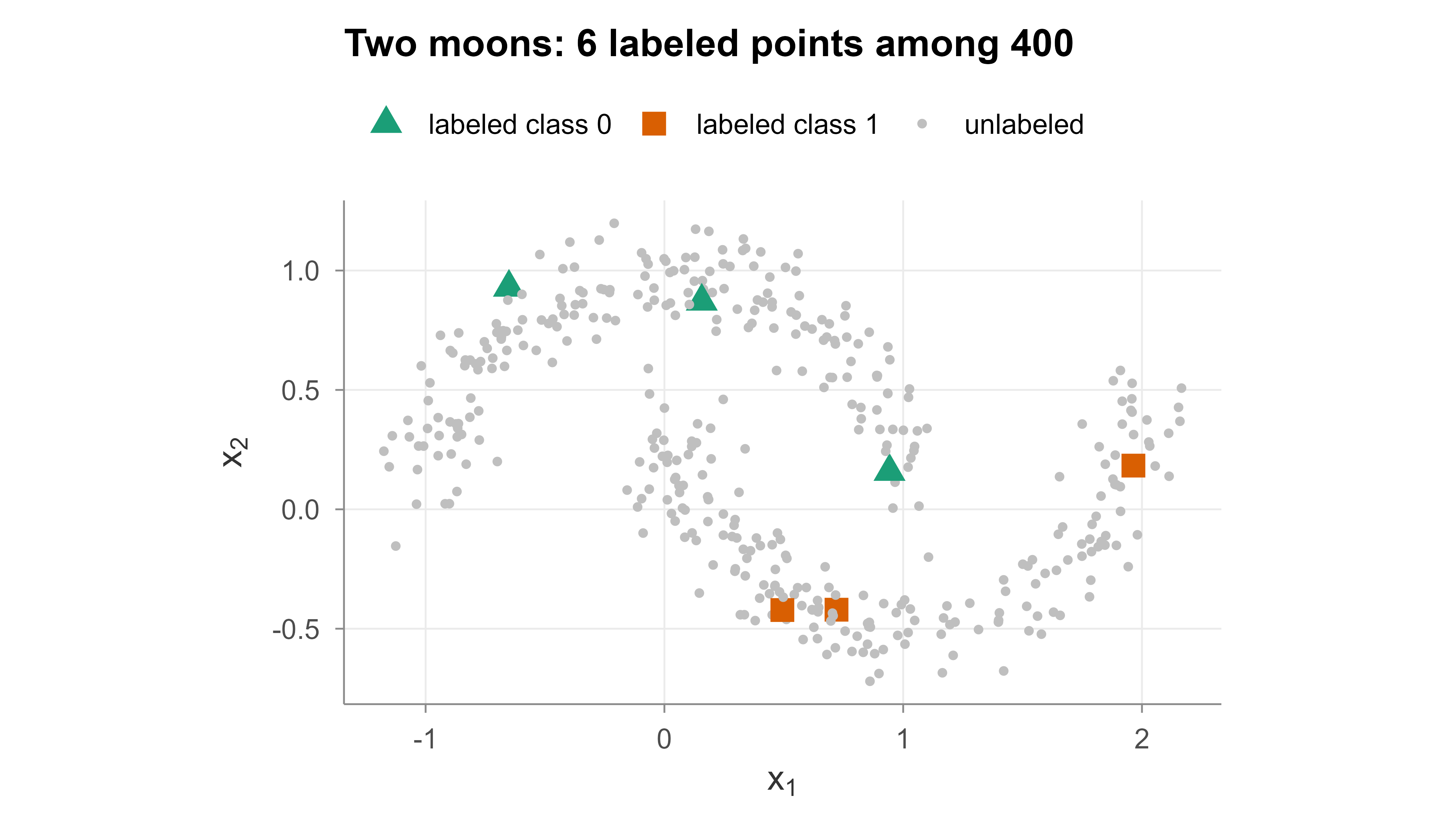
library(ggplot2)

plot_df <- data.frame(
  x1 = X[, 1], x2 = X[, 2],
  status = ifelse(y_obs == -1, "unlabeled",
                  ifelse(y_obs == 0, "labeled class 0", "labeled class 1"))
)

ggplot(plot_df, aes(x1, x2)) +
  geom_point(aes(color = status, size = status, shape = status)) +
  scale_color_manual(values = c("unlabeled" = "grey75",
                                "labeled class 0" = "#1b9e77",
                                "labeled class 1" = "#d95f02")) +
  scale_size_manual(values = c("unlabeled" = 1.2,
                               "labeled class 0" = 3.5,
                               "labeled class 1" = 3.5)) +
  scale_shape_manual(values = c("unlabeled" = 16,
                                "labeled class 0" = 17,
                                "labeled class 1" = 15)) +
  labs(title = "Two moons: 6 labeled points among 400",
       x = expression(x[1]), y = expression(x[2]),
       color = NULL, size = NULL, shape = NULL) +
  coord_equal()

Figure 48.1: Two-moons dataset with 6 labeled points (large triangle and square markers) among 400 total points (grey dots are unlabeled). The two classes form interleaved crescents that lie on clear one-dimensional manifolds.

Figure 48.1 shows the difficulty: with only six labels, a supervised method has almost nothing to anchor the boundary. But the unlabeled points trace out two clear crescents, and the graph methods will exploit that shape.

48.9.1 Building the graph and propagating

We build a Gaussian-kernel similarity matrix, restrict it to \(k\) nearest neighbors for sparsity, and run both the clamped (label propagation) and soft-clamp (label spreading) closed-form solutions.

# Pairwise squared Euclidean distances.
sq_dist <- as.matrix(dist(X))^2

# k-nearest-neighbor Gaussian weights (symmetrized).
knn_gaussian_W <- function(D2, k = 10, sigma = NULL) {
  n <- nrow(D2)
  if (is.null(sigma)) {
    # median heuristic on nonzero distances
    sigma <- sqrt(median(D2[D2 > 0]))
  }
  Wfull <- exp(-D2 / (2 * sigma^2))
  W <- matrix(0, n, n)
  for (i in seq_len(n)) {
    ord <- order(D2[i, ])
    nbrs <- ord[2:(k + 1)]          # skip self
    W[i, nbrs] <- Wfull[i, nbrs]
  }
  W <- pmax(W, t(W))                # symmetrize
  diag(W) <- 0
  W
}

W <- knn_gaussian_W(sq_dist, k = 10)
D <- rowSums(W)

# One-hot label matrix Y (n x C); unlabeled rows are all zero.
C <- 2
Y <- matrix(0, n, C)
for (i in lab_idx) Y[i, y_obs[i] + 1L] <- 1

L <- which(y_obs != -1)
Uidx <- which(y_obs == -1)

# --- Label propagation: harmonic solution with clamped labels ---
# F_U = (I - P_UU)^{-1} P_UL Y_L,  where P = D^{-1} W.
P <- W / D                                  # row-normalized transition matrix
P_UU <- P[Uidx, Uidx]
P_UL <- P[Uidx, L]
F_U  <- solve(diag(length(Uidx)) - P_UU, P_UL %*% Y[L, , drop = FALSE])

pred_lp <- rep(NA_integer_, n)
pred_lp[L]    <- y_obs[L]
pred_lp[Uidx] <- max.col(F_U) - 1L

# --- Label spreading: F* = (1 - alpha)(I - alpha S)^{-1} Y ---
alpha <- 0.99
Dinv_sqrt <- 1 / sqrt(D)
S <- (Dinv_sqrt) * W * rep(Dinv_sqrt, each = n)   # D^{-1/2} W D^{-1/2}
F_star <- (1 - alpha) * solve(diag(n) - alpha * S, Y)

pred_ls <- max.col(F_star) - 1L

# --- Supervised baseline: 1-NN trained on the 6 labeled points only ---
nn_predict <- function(Xtr, ytr, Xte) {
  apply(Xte, 1, function(q) {
    d <- colSums((t(Xtr) - q)^2)
    ytr[which.min(d)]
  })
}
pred_nn <- nn_predict(X[L, , drop = FALSE], y_obs[L], X)

48.9.2 Verifying the closed form against the iteration

The derivation claimed that the clamped random-walk iteration \(F_U^{(t+1)} = P_{UU} F_U^{(t)} + P_{UL} Y_L\) converges to the closed form Equation 48.4. We confirm this numerically by iterating from a zero initialization and comparing to the matrix-inverse solution.

# Convergence rate is set by the spectral radius of P_UU.
rho <- max(abs(eigen(P_UU, only.values = TRUE)$values))

# Iterate the clamped update from F_U = 0 and compare to the closed form.
F_iter <- matrix(0, length(Uidx), C)
for (t in 1:5000) {
  F_iter <- P_UU %*% F_iter + P_UL %*% Y[L, , drop = FALSE]
}
max_abs_diff <- max(abs(F_iter - F_U))
labels_match <- all(max.col(F_iter) == max.col(F_U))

cat("Spectral radius rho(P_UU):", round(rho, 4), "\n")
#> Spectral radius rho(P_UU): 0.9948
cat("Max |iteration - closed form| after 5000 steps:",
    format(max_abs_diff, scientific = TRUE), "\n")
#> Max |iteration - closed form| after 5000 steps: 7.633338e-12
cat("Predicted labels identical:", labels_match, "\n")
#> Predicted labels identical: TRUE

The iterate matches the closed form Equation 48.4 to within machine precision, confirming that the recursion and the matrix inverse compute the same harmonic solution. The spectral radius \(\rho(P_{UU})\) is close to 1 here (a few unlabeled nodes sit far from any label, so probability mass leaks to the absorbing set only slowly), which is why thousands of iterations are needed for full numerical agreement even though the predicted labels, the argmax of each row, stabilize after only a few hundred. This is the linear convergence rate \(\rho(P_{UU})\) from the Neumann-series argument made concrete: the closed form is the better choice at this scale precisely because the iteration converges slowly when the graph is weakly absorbing.

48.9.3 Accuracy gain from unlabeled data

We score each method on the points that were hidden during training (the unlabeled set), which is the fair comparison: did using the unlabeled structure help recover the true labels?

acc_on_U <- function(pred) mean(pred[Uidx] == y_true[Uidx])

results <- data.frame(
  method = c("Supervised 1-NN (labels only)",
             "Label propagation (clamped)",
             "Label spreading (soft clamp)"),
  uses_unlabeled = c("no", "yes", "yes"),
  accuracy_on_unlabeled = round(
    c(acc_on_U(pred_nn), acc_on_U(pred_lp), acc_on_U(pred_ls)), 3
  )
)

knitr::kable(
  results,
  caption = "Accuracy on the held-out unlabeled points. The supervised baseline sees only the six labels; the graph methods also use the 394 unlabeled points to trace the manifold."
)

Table 48.2: Accuracy on the held-out unlabeled points. The supervised baseline sees only the six labels; the graph methods also use the 394 unlabeled points to trace the manifold.

method	uses_unlabeled	accuracy_on_unlabeled
Supervised 1-NN (labels only)	no	0.939
Label propagation (clamped)	yes	0.995
Label spreading (soft clamp)	yes	0.995

Table 48.2 reports the result. The supervised 1-NN has only six reference points, so it splits the plane by raw distance and misclassifies large stretches of each crescent. The graph methods diffuse the six labels along the two arcs and recover almost all of the hidden labels. The gap between the rows is the accuracy gain attributable to the unlabeled data.

48.9.4 Visualizing the propagated labels

res_df <- data.frame(
  x1 = X[, 1], x2 = X[, 2],
  predicted = factor(pred_lp, levels = c(0, 1)),
  is_labeled = y_obs != -1
)

ggplot(res_df, aes(x1, x2)) +
  geom_point(aes(color = predicted), size = 1.4, alpha = 0.8) +
  geom_point(data = subset(res_df, is_labeled),
             shape = 21, fill = NA, color = "black",
             size = 4, stroke = 1.1) +
  scale_color_manual(values = c("0" = "#1b9e77", "1" = "#d95f02")) +
  labs(title = "Labels after propagation (circled points were the 6 given labels)",
       x = expression(x[1]), y = expression(x[2]), color = "predicted") +
  coord_equal()

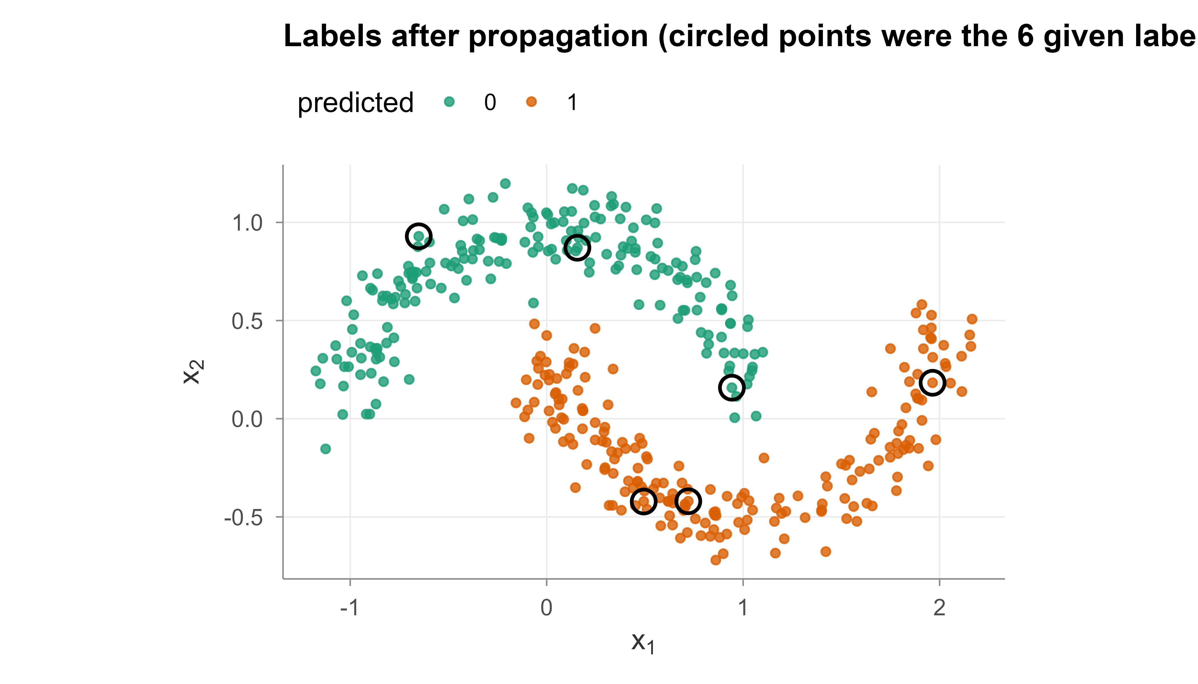
Figure 48.2: Predicted labels after label propagation. Each point is colored by its propagated class, and the black circles mark the 6 originally labeled points. Both crescents are recovered, showing that propagation followed the manifold rather than straight-line distance.

Figure 48.2 shows the outcome: each crescent is now colored consistently, even though only three labels per class were given. The black circles mark the original labeled points. Propagation followed the manifold rather than raw straight-line distance, which is exactly what the manifold assumption promises.

Key idea

Six labels were nowhere near enough for the supervised baseline, yet they were plenty once the 394 unlabeled points revealed the two crescents. That is the entire SSL bargain in one picture: unlabeled data supplies the shape, and a few labels supply the names.

48.10 Practical Guidance

Methods are only half the story; knowing when to apply them is the other half. The conditions below tell you when SSL is likely to pay off.

48.10.1 When to use semi-supervised learning

SSL tends to help when all three of the following hold:

• You have far more unlabeled than labeled data, and labeling is the expensive step.
• The cluster or manifold assumption is plausible for your data. Check this: if a quick unsupervised view (clustering, a 2-D projection) shows class-coherent structure, SSL is likely to help.
• The unlabeled data comes from the same distribution as the labeled data and the eventual test data. Distribution shift between \(L\) and \(U\) breaks the premise.

48.10.2 When to be cautious

By the same token, hold off when any of these warning signs appear:

• Labels are abundant relative to the problem’s complexity. Once you have enough labeled data, adding unlabeled data yields little and can hurt.
• The assumptions fail. If classes overlap in dense regions, low-density separation pushes the boundary to the wrong place. SSL is not free; the negative-result literature shows unlabeled data can degrade performance when the model of \(p(x)\) is wrong.
• You cannot validate. SSL has hyperparameters (the threshold \(\tau\), the graph bandwidth \(\sigma\), the neighbor count \(k\), the spreading weight \(\alpha\)) that need a labeled validation set or principled defaults.

48.10.3 Pitfalls and how to manage them

When you do apply SSL, a handful of recurring traps account for most failures. Each one below pairs the problem with a concrete remedy:

• Confirmation bias in self-training. Use a high confidence threshold, add few points per round, and re-evaluate pseudo-labels each round instead of freezing them. Consider class-balanced selection so the majority class does not swamp the pseudo-labels.
• Graph construction dominates results. The choice of \(\sigma\), \(k\), and the distance metric matters more than the diffusion algorithm. Standardize features first (distances are scale-sensitive), and tune \(\sigma\) with a heuristic like the median pairwise distance, then refine on validation labels.
• Computational cost. The closed-form graph solutions invert an \(n \times n\) (or \(u \times u\)) matrix, \(O(n^3)\) in general. For large \(n\) use the iterative form, exploit sparsity from \(k\)-NN graphs, or use scalable approximations.
• Calibration. Confidence-based methods assume the model’s probabilities mean something. Poorly calibrated models pseudo-label badly; calibrate (for example with temperature scaling) before thresholding.
• Validation must use real labels. Never tune on pseudo-labels; that measures self-consistency, not accuracy. Hold out a genuinely labeled validation set.

48.10.4 Computational complexity and scaling

The graph methods have a clear cost profile. Building the full Gaussian kernel is \(O(n^2 p)\) time and \(O(n^2)\) memory; restricting to a \(k\)-NN graph (exact brute force) keeps the \(O(n^2 p)\) distance computation but reduces storage to \(O(nk)\), and approximate nearest-neighbor structures (KD-trees in low dimension, or locality-sensitive hashing and HNSW graphs in high dimension) bring the construction toward \(O(n \log n)\) in favorable regimes. The solve is the bottleneck. The direct closed forms Equation 48.4 and Equation 48.6 invert a dense \(u \times u\) or \(n \times n\) system at \(O(u^3)\) or \(O(n^3)\), which is fine for the few thousand points of the simulation but infeasible past tens of thousands. Two scalable routes exist:

• Iterative solves. Run the fixed-point recursions (the clamped update, or \(F \leftarrow \alpha S F + (1-\alpha) Y\)) on the sparse \(k\)-NN matrix. Each iteration costs \(O(nk C)\), and convergence to tolerance \(\varepsilon\) takes \(O\!\big(\log \varepsilon / \log \rho\big)\) iterations, where \(\rho\) is the relevant spectral radius (\(\rho(P_{UU})\) or \(\alpha\)). Total cost is near-linear in \(n\) for a fixed graph. Conjugate gradient on the symmetric positive-definite systems converges faster when the graph is well conditioned.
• Anchor and Nystrom approximations. Summarize the graph by \(m \ll n\) landmark points and propagate through the landmarks, reducing the solve to \(O(m^3 + nm)\).

For self-training and pseudo-labeling the cost is dominated by the repeated retraining: \(R\) rounds times the base learner’s training cost. Re-evaluating (not freezing) pseudo-labels each round, recommended against confirmation bias, multiplies inference cost over \(U\) by \(R\) but does not change the asymptotic order.

48.10.5 Choosing the bandwidth and neighbor count

Distances must be on a sensible scale, so standardize or whiten features before building the graph. For the bandwidth \(\sigma\), the median heuristic used in the simulation (set \(\sigma\) to the median pairwise distance, or to the median distance to the \(k\)-th neighbor for a local version) is a robust default that adapts to the data scale. Refine it on a labeled validation fold by grid search over a small multiplicative range, since accuracy is typically a smooth, single-peaked function of \(\sigma\). For \(k\), values in the range 5 to 20 are standard; too small fragments the graph into disconnected pieces (so some unlabeled nodes have no path to a label and Equation 48.4 has no unique solution on that component), while too large blurs the manifold by connecting across the low-density gap, which defeats the whole purpose. A useful diagnostic is to check the number of connected components of the \(k\)-NN graph: it should be small and ideally equal to (or fewer than) the number of classes.

48.10.6 Inductive use

Label propagation and spreading label only the points you give them. To predict on new data, either rebuild the graph including the new points and rerun (transductive), or train a standard supervised model on the now-labeled set and use it inductively. The second route is common in production: SSL is the labeling engine, and a fast supervised model is the deployed predictor.

Tip

In a deployed system, do not put a graph method on the serving path. Run it offline to manufacture labels, then train a lightweight inductive model (logistic regression, a gradient-boosted tree (Chapter 12), a small network) on the enlarged labeled set and ship that. You get the labeling benefit of SSL with the latency of an ordinary classifier.

48.11 Further Reading

To go deeper, the references below trace the field from its founding algorithms to modern deep-learning practice. The first three are the original papers behind the methods in this chapter; the last three are surveys and edited volumes that give the wider map.

• Blum, A. and Mitchell, T. (1998). Combining labeled and unlabeled data with co-training. The original co-training algorithm and its theory under the view-independence assumption.
• Zhu, X. and Ghahramani, Z. (2002). Learning from labeled and unlabeled data with label propagation. The harmonic label-propagation method on graphs.
• Zhou, D., Bousquet, O., Lal, T. N., Weston, J., and Schölkopf, B. (2004). Learning with local and global consistency. The label-spreading method with the normalized Laplacian and soft clamping.
• Chapelle, O., Schölkopf, B., and Zien, A. (eds.) (2006). Semi-Supervised Learning. A comprehensive reference covering the cluster and manifold assumptions, graph methods, and low-density separation.
• Zhu, X. and Goldberg, A. B. (2009). Introduction to Semi-Supervised Learning. A concise, readable survey of the main method families.
• van Engelen, J. E. and Hoos, H. H. (2020). A survey on semi-supervised learning. A modern overview that connects classic methods to deep pseudo-labeling and consistency regularization.

---

1. A wrapper method is one that sits on top of any existing supervised learner, treating it as a black box. You do not modify the classifier’s internals; you only change the data you feed it.

2. Conditionally independent given the label means that once you know the class, the two views carry no extra information about each other. This is what stops the two classifiers from making the same mistakes.

3. Small \(\sigma\) makes the kernel pick out only very close neighbors (a tight, local graph); large \(\sigma\) connects far-apart points too (a loose, global graph). This single number has more influence on the result than the choice of diffusion algorithm.

4. The graph Laplacian is the discrete analogue of the second-derivative operator from calculus. Just as the second derivative measures how much a function curves, the Laplacian measures how much a labeling disagrees across edges, which is exactly the smoothness the manifold assumption wants to minimize.