Imagine you are trying to draw a smooth curve through a cloud of scattered points, with no formula in mind for the shape of that curve. Kernel smoothing (Chapter 4) gives one answer: at each point of interest, average the nearby observations, weighting closer neighbors more heavily. That works well in the middle of the data, but it stumbles near the edges. At a boundary, all of your neighbors sit on one side, so a simple weighted average is pulled inward and the fitted curve bends away from the truth. Local regression fixes this by replacing the local average with a local line: instead of asking “what is the typical \(y\) near here?”, it asks “what straight line best describes the data near here?” A line can tilt to follow a trend that runs off the edge of the data, so it corrects the boundary problem that plagues plain kernel smoothing.
This chapter shows how that idea is made precise, how it extends to higher-degree polynomials and to more than one predictor, and how to fit it in R with loess. By the end you should understand why local linear fits are the workhorse choice, when a local quadratic fit earns its extra variance, and why the whole approach quietly breaks down once you have more than a few predictors.
Key idea
Local regression fits a simple model (a line, or a low-degree polynomial) inside a moving neighborhood, weighting points by how close they are. The fitted value at a point is read off that local model. Sliding the neighborhood across the range of \(x\) traces out a smooth curve.
This method is also known as locally weighted linear regression, and the most common software implementation is called loess (or lowess).
5.1 From local averages to local lines
At a target point \(x_0\), local linear regression solves a weighted least squares problem: it fits a line to the data, but down-weights observations far from \(x_0\) using the kernel weights \(K_\lambda(x_0, x_i)\) (the same neighborhood weights from kernel smoothing (Chapter 4), where \(\lambda\) controls how wide the neighborhood is). Formally, it seeks
and gives the estimate \(\hat{f}(x_0) =\hat{\alpha}(x_0)+ \hat{\beta}(x_0)x_0\).
Notice that the intercept \(\alpha(x_0)\) and slope \(\beta(x_0)\) both carry the argument \(x_0\): we are not fitting one global line but a fresh line at every target point. The fitted value is then this local line evaluated back at \(x_0\).
Intuition
A weighted average is just a local fit of a constant. Local linear regression upgrades that constant to a line. Because a line can have a nonzero slope, it can follow a trend right up to the edge of the data, which is exactly where a flat local average goes wrong.
It is worth writing the solution in matrix form, because it reveals something useful. Let \(b(x)^T = (1,x)\) collect the intercept-and-slope basis, and define the \(n \times 2\) matrix \(\mathbf{B}\) whose \(i\)-th row is \(b(x_i)^T\). Let \(\mathbf{W}(x_0)\) be the \(n \times n\) diagonal matrix whose \(i\)-th diagonal entry is the kernel weight \(K_\lambda(x_0, x_i)\). Then the weighted least squares solution is
The right-hand side is the payoff: the fitted value is a linear combination of the observed \(y_i\), with weights \(l_i(x_0)\) that depend only on the \(x\) values and the kernel, not on the responses. These weights blend the kernel weights with the least squares machinery, and the resulting weighting function is called the equivalent kernel.1
5.1.1 Deriving the weighted least squares solution
It is worth seeing where the matrix formula comes from, because the derivation is short and it makes the structure of \(l_i(x_0)\) explicit. Fix the target \(x_0\) and abbreviate \(\beta = (\alpha(x_0), \beta(x_0))^T\) and \(w_i = K_\lambda(x_0, x_i)\). The objective is
Expanding gives \(J(\beta) = \mathbf{y}^T\mathbf{W}\mathbf{y} - 2\beta^T \mathbf{B}^T\mathbf{W}\mathbf{y} + \beta^T \mathbf{B}^T\mathbf{W}\mathbf{B}\,\beta\). Differentiating with respect to \(\beta\) and setting the gradient to zero,
The Hessian \(\partial^2 J/\partial\beta\partial\beta^T = 2\,\mathbf{B}^T\mathbf{W}\mathbf{B}\) is positive definite whenever \(\mathbf{W}\) has at least two strictly positive weights at distinct design points, so the stationary point is the unique global minimum. Reading the fit at \(x_0\) gives \(\hat{f}(x_0) = b(x_0)^T\hat{\beta}(x_0)\), and collecting the row vector that multiplies \(\mathbf{y}\),
so \(\hat{f}(x_0) = \sum_i l_i(x_0) y_i\) as claimed. The weights in Equation 5.3 are the equivalent kernel.
5.1.2 Why local linear fits reproduce lines: the moment conditions
The equivalent kernel satisfies discrete moment conditions that explain the boundary-bias correction directly. Because the local fit is the projection of \(\mathbf{y}\) onto the column space of \(\mathbf{B}\) in the \(\mathbf{W}\)-inner product, it reproduces any function that lies in that column space exactly. Concretely, for \(\hat{f}(x_0) = \sum_i l_i(x_0) y_i\), substituting \(y_i = b(x_i)^T c\) for any fixed coefficient vector \(c\) recovers \(b(x_0)^T c\), which forces
for the local linear basis \(b(x)^T = (1, x)\) (and, more generally, \(\sum_i (x_i - x_0)^j l_i(x_0) = 0\) for \(j = 1, \dots, d\) at polynomial degree \(d\)). The first condition says the weights sum to one, so constants pass through untouched. The second condition is the one a plain kernel average lacks: it says the equivalent kernel has zero first moment, so a linear trend also passes through untouched, even at a boundary where the raw kernel weights are lopsided. This is the precise sense in which “the line can tilt to follow the trend off the edge.”
Note
Because \(\hat{f}(x_0) = \sum_i l_i(x_0) y_i\) is linear in \(\mathbf{y}\), local regression is a linear smoother. That linearity makes quantities like effective degrees of freedom and pointwise standard errors easy to compute, just as in ordinary linear regression.
The advantage of moving from constants to lines is concrete: local linear regression corrects the boundary bias to first order, meaning the leading bias term now depends only on the second derivative of \(f\) and so is small on average. The price is small. The fit tends to be slightly biased in regions where the true function curves sharply, because a straight line cannot bend.
5.1.3 Bias and variance of the local linear estimator
The moment conditions in Equation 5.4 translate into a clean expansion of the bias, which is what makes the boundary claim rigorous. Assume the model \(y_i = f(x_i) + \varepsilon_i\) with \(\mathbb{E}[\varepsilon_i] = 0\), \(\operatorname{Var}(\varepsilon_i) = \sigma^2\), and independent errors. Conditioning on the design, the estimator \(\hat{f}(x_0) = \sum_i l_i(x_0) y_i\) is linear, so
To get the bias, expand \(f\) around \(x_0\) in a Taylor series, \(f(x_i) = f(x_0) + f'(x_0)(x_i - x_0) + \tfrac12 f''(x_0)(x_i - x_0)^2 + o((x_i - x_0)^2)\), and substitute into Equation 5.5. The constant term contributes \(f(x_0)\sum_i l_i(x_0) = f(x_0)\) by the first moment condition, and the linear term contributes \(f'(x_0)\sum_i (x_i - x_0) l_i(x_0) = 0\) by the second. Both vanish, leaving
so the leading bias is proportional to \(f''(x_0)\) and to the kernel’s second moment, and it carries no contribution from \(f'\). This is exactly why a sharp slope near a boundary does not bias a local linear fit, while it does bias a local average (whose equivalent kernel violates the second moment condition). For a kernel of bandwidth \(h\) in the interior, \(\sum_i (x_i - x_0)^2 l_i(x_0) = O(h^2)\) and \(\|l(x_0)\|^2 = O(1/(nh))\), giving the canonical one-dimensional rates
Minimizing the pointwise mean squared error \(\text{bias}^2 + \text{variance} = O(h^4) + O(1/(nh))\) over \(h\) balances the two terms at \(h \asymp n^{-1/5}\), yielding the optimal MSE rate \(O(n^{-4/5})\). This is the standard nonparametric rate for estimating a twice-differentiable function in one dimension, and it is slower than the parametric \(O(n^{-1})\), the price of not assuming a global form for \(f\).
Note
The variance factor \(\|l(x_0)\|^2 = \sum_i l_i(x_0)^2\) is computable directly from the smoother weights and needs no knowledge of \(f\). It is the basis for the pointwise standard error bands that loess and predict report: \(\widehat{\operatorname{se}}(\hat{f}(x_0)) = \hat\sigma\,\|l(x_0)\|\), with \(\hat\sigma^2\) estimated from the residuals.
5.1.4 Effective degrees of freedom
Stacking the equivalent-kernel rows for the \(n\) fitted values gives the smoother matrix \(\mathbf{L}\), whose \(i\)-th row is \(l(x_i)^T\), so that \(\hat{\mathbf{f}} = \mathbf{L}\mathbf{y}\). By analogy with the hat matrix of ordinary regression, where the trace counts parameters, the effective degrees of freedom of a linear smoother are defined as
A small span makes each local fit hug its own observation, pushing \(l_i(x_i)\) toward one and \(\mathrm{df}\) toward \(n\) (a wiggly, high-variance fit); a large span spreads the weights and shrinks \(\mathrm{df}\) toward the number of local parameters (a smooth, stiff fit). This single number summarizes model complexity and feeds directly into the model-selection criteria below. In R, loess reports it as the trace.hat-based equivalent number of parameters in summary(fit).
5.2 Going to higher-degree polynomials
If a line cannot bend and the bias from curvature bothers you, the natural next step is to let the local model bend by fitting a low-degree polynomial instead. This is local polynomial regression (with local quadratic regression as the common case, \(d = 2\)):
which gives the solution \(\hat{f}(x_0) = \hat{\alpha}(x_0)+ \sum_{j=1}^d \hat{\beta}_j(x_0)x_0^j\).
A quadratic can curve to match a peak or a valley, so it reduces the bias in curved regions. That reduction is not free: estimating more local coefficients from the same handful of nearby points inflates the variance. This bias-variance trade-off is the central tension in choosing the polynomial degree.
The accumulated wisdom on which degree to use can be summarized in a few rules of thumb:
Local linear fits (\(d=1\)) handle the boundaries far better than higher-order polynomials, and they do so without a large variance penalty.
Local quadratic fits (\(d=2\)) buy little at the boundaries but pay a steep variance cost there.
Local quadratic fits earn their keep in the interior, where they trim the bias caused by curvature in the true function.
Asymptotically, local polynomials of odd degree dominate those of even degree, because asymptotic mean squared error is dominated by boundary effects, where the odd-degree fits do better.
The odd-degree advantage has a clean explanation through the moment conditions. A local polynomial of degree \(d\) forces the equivalent kernel to have zero moments up to order \(d\) (the generalization of Equation 5.4), so by the Taylor argument of Section 5.1.3 the leading bias is governed by the \((d+1)\)-th moment \(\sum_i (x_i - x_0)^{d+1} l_i(x_0)\) times \(f^{(d+1)}(x_0)\). In the interior, where the design is locally symmetric about \(x_0\), all odd moments of the equivalent kernel vanish by symmetry. For even \(d\) this is no help, the bias is already set by the order-\((d+1)\) (odd) moment, but for odd \(d\) the order-\((d+1)\) moment is even and nonzero while the next odd moment is killed by symmetry, so going from \(d = 2m\) to \(d = 2m+1\) removes a variance penalty (one fewer parameter than the next even degree at the same bias order) without adding bias order. The practical consequence is that \(d = 1\) and \(d = 3\) are the sensible choices, and \(d = 1\) is the default.
When to use this
Reach for local linear regression by default. Step up to local quadratic only when you have reason to believe the true function curves sharply in the interior of the data and you have enough observations there to absorb the extra variance.
5.3 Higher Dimensions
Everything so far assumed a single predictor. To generalize kernel smoothing (Chapter 4) and local regression to \(p\) predictors, we fit local hyperplanes (or local polynomial surfaces) using a \(p\)-dimensional kernel. The only real change is bookkeeping in the basis \(b(X)\).
To make the basis concrete, here are two small cases (\(d\) is the polynomial degree, \(p\) the number of predictors):
With \(d= 1\) and \(p=2\), the basis is \(b^T(X) = (1,X_1,X_2)\), a local plane.
With \(d =2\) and \(p=2\), the basis is \(b^T(X) = (1, X_1, X_2, X_1^2, X_2^2, X_1 X_2)\), a local quadratic surface including the interaction term.
With the basis chosen, we solve the same weighted least squares problem as before, now with vector-valued inputs:
where \(||.||\) is the Euclidean norm and \(D\) is a one-dimensional weighting function applied to that distance.
Warning
The Euclidean norm mixes all coordinates together, so it is sensitive to the scale of each variable. A predictor measured in thousands will dominate one measured in fractions. Standardize the predictors before fitting, or the neighborhoods will be defined almost entirely by the large-scale variables.
Higher dimensions make the boundary problem worse, not better. Because of the curse of dimensionality, as \(p\) grows a larger and larger fraction of the data sits on or near the boundary of the predictor space, so the very region where local fits struggle becomes most of the region.2 As in one dimension, local polynomial regression still corrects this boundary bias to first order, but the deeper difficulty is balancing localness (which lowers bias) against variance as \(p\) climbs, all without the exponentially larger sample size that true localness in high dimensions would demand.
Warning
As a practical rule, do not use kernel smoothing or local polynomial regression in more than about three dimensions. Beyond that, the neighborhoods are either too sparse (high variance) or too wide to be local (high bias), and structured methods such as generalized additive models (Chapter 6) are needed.
5.3.1 Adding structure when dimension is high
When the ratio of dimension to sample size is high, the way out is to impose structure that restricts how the function can vary, trading some flexibility for stability. Two strategies are common.
The first is to reshape the distance used inside the kernel. Instead of the plain Euclidean norm, use a quadratic form with a matrix \(\mathbf{A}\):
where \(\mathbf{A}\) is a \(p \times p\) positive semi-definite matrix. By choosing \(\mathbf{A}\) you can give different weights to different directions, or recombine coordinates to shrink (“compress”) whole dimensions, effectively flattening the neighborhood along directions where the function changes little (a goal closely related to dimension reduction, Chapter 27).
The second strategy adds structure through varying coefficient models. Suppose you split the \(p\) inputs into two groups: the first \(q\) variables enter a linear regression, but their coefficients are allowed to depend on the remaining inputs \(Z= (X_{q+1}, X_{q+2}, \dots, X_p)\). The model is
so the relationship between \(Y\) and \(X_1, \dots, X_q\) is linear, but its intercept and slopes drift smoothly as \(Z\) changes.3 We estimate the coefficient functions by kernel-weighted local regression in the \(Z\) space:
Both tricks fight the curse of dimensionality the same way: by refusing to let the function vary freely in every direction at once. Reshaping the kernel limits where the model looks; varying coefficient models limit how the model is allowed to bend.
5.4 Application
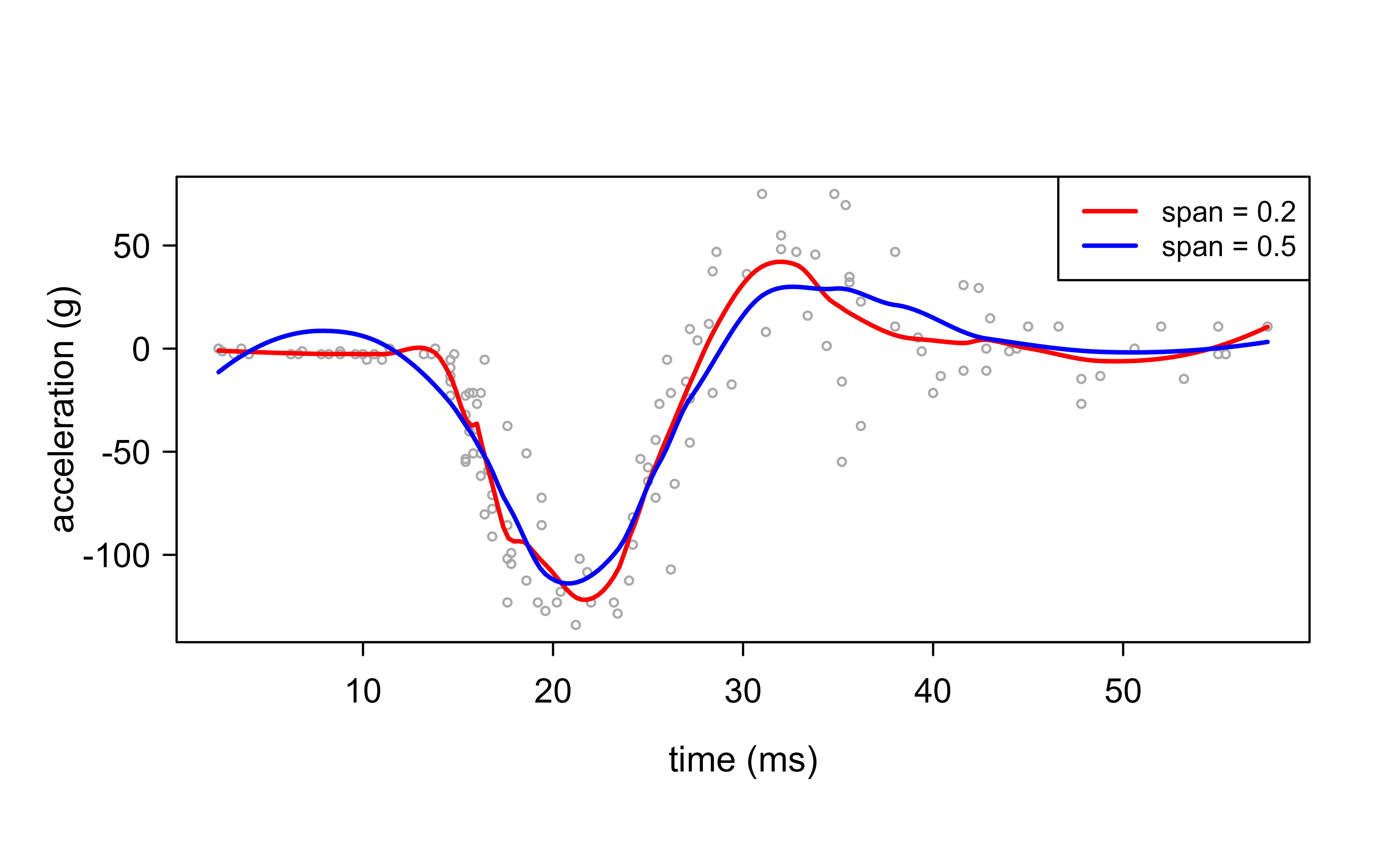
We fit local regression in R with loess to mcycle (in MASS), a classic nonparametric-regression benchmark: head acceleration measured through a simulated motorcycle crash. The signal is sharply nonlinear and the noise level changes across the range, so it is an honest test of a smoother. The one tuning parameter is span, the fraction of observations in each local neighborhood: a larger span averages more neighbors (smoother, lower variance), a smaller span follows the data closely (wigglier, higher variance).4
We overlay a narrow (span = 0.2) and a wide (span = 0.5) fit so the bias-variance effect is visible directly:
Show code
data(mcycle, package ="MASS")grid<-data.frame(times =seq(min(mcycle$times), max(mcycle$times), length.out =200))plot(mcycle$times, mcycle$accel, cex =.5, col ="darkgrey", xlab ="time (ms)", ylab ="acceleration (g)")f02<-loess(accel~times, span =0.2, data =mcycle)f05<-loess(accel~times, span =0.5, data =mcycle)lines(grid$times, predict(f02, grid), col ="red", lwd =2)lines(grid$times, predict(f05, grid), col ="blue", lwd =2)legend("topright", c("span = 0.2", "span = 0.5"), col =c("red", "blue"), lty =1, lwd =2, cex =0.8)
Figure 5.1: Local regression of head acceleration on time, span 0.2 (red) versus 0.5 (blue). The wider span is smoother but lags the sharp dip; the narrower one tracks it at the cost of more wiggle.
Eyeballing two fits is not a selection rule, though. The span is the bias-variance dial, so choose it the way the theory says — by minimizing honest held-out error. A 10-fold cross-validation over a grid of spans traces the U-shaped risk curve and names the winner:
The error is flat-to-best at the small spans and then climbs steeply as the neighborhood widens — oversmoothing erases the very dip that matters, so the cross-validated RMSE more than half again worse at span = 0.9 than at the optimum near span = 0.3. This is the same lesson as the kernel bandwidth (Section 4.2) in a different costume: the smoother shape barely matters, the amount of smoothing is everything, and you set it by cross-validation rather than by eye.
The red curve (span = 0.2) wiggles to track local features in the data, while the blue curve (span = 0.5) is noticeably smoother because each fitted point borrows strength from a wider neighborhood. This single picture captures the bias-variance trade-off that runs through the whole chapter: widen the neighborhood to reduce variance and you risk smoothing away real structure, narrow it to reduce bias and you let noise back into the fit. Choosing the span (by cross-validation or by judgment) is therefore the central practical decision when using local regression.
5.4.1 Choosing the span
The span plays the role of the bandwidth \(h\) from Section 5.1.3, but loess parameterizes it as the fraction of observations in each neighborhood, which makes the bandwidth adapt to the local data density (nearest-neighbor bandwidth). Three principled routes to a value exist.
The first is leave-one-out cross-validation. Because local regression is a linear smoother, the leave-one-out residuals have the closed form that avoids refitting,
where \(L_{ii} = l_i(x_i)\) is the \(i\)-th diagonal of the smoother matrix (the leverage), exactly as in ordinary least squares. The whole CV curve over a grid of spans costs only the diagonal of \(\mathbf{L}\) per fit, not \(n\) separate refits.
The second is generalized cross-validation, which replaces each \(L_{ii}\) by the average \(\operatorname{tr}(\mathbf{L})/n = \mathrm{df}/n\),
The third is an AIC-type criterion that penalizes the residual sum of squares by the effective degrees of freedom from Equation 5.8; fANCOVA::loess.as automates span selection by AICc or GCV and is the convenient choice in practice. All three trade the same quantities: smaller span lowers the residual sum of squares but raises \(\mathrm{df}\), and the criterion picks the span where the marginal reduction in fit error no longer pays for the added complexity.
Computational cost
A single fit at one target costs \(O(n_h\, p^2 + p^3)\), the weighted cross-products over the \(n_h\) neighbors plus a \((p\!+\!1)\!\times\!(p\!+\!1)\) solve, where \(n_h = \text{span}\times n\). Naively evaluating all \(n\) targets is \(O(n \cdot n_h)\), which is quadratic when the span is a fixed fraction. loess avoids this by fitting exactly at the vertices of a \(k\)-d tree and interpolating elsewhere (the surface = "interpolate" default), which is what makes it fast on large \(n\). Set surface = "direct" to fit at every point when you need exact values, accepting the higher cost.
The leverage identity behind Equation 5.9 is easy to confirm directly from a loess fit, which also verifies that the equivalent kernel and effective degrees of freedom are exactly the trace-based quantities defined above.
Show code
# Verify df = tr(L) by reconstructing the smoother matrix column by column:# fitting loess on the i-th unit vector returns the i-th column of L.n<-length(age)ord<-order(age)fit_unit<-function(j){e<-numeric(n); e[j]<-1predict(loess(e~age, span =0.5, degree =1, control =loess.control(surface ="direct")))}L<-sapply(seq_len(n), fit_unit)# n x n smoother matrix, hat = Ldf_from_trace<-sum(diag(L))df_reported<-loess(wage~age, span =0.5, degree =1)$trace.hatc(trace =df_from_trace, reported =df_reported)# should match closely
The equivalent kernel is a helpful diagnostic: it tells you, for a given target point, exactly how much each observation contributes to the fit. Near a boundary it automatically reshapes itself so that the fit stops being dragged inward, which is the mathematical reason local linear fits beat local averages at the edges.↩︎
A quick way to feel this: in a unit hypercube, the fraction of volume within a thin shell of the surface grows toward 1 as the dimension increases. Almost every point is “near an edge” in high dimensions.↩︎
A familiar example: a regression of spending on income whose slope changes with age. The model is linear in income at any fixed age, but the income effect itself varies across the age dimension.↩︎
An alternative is the locfit package, which offers adaptive bandwidths and more control over the local degree. We use base loess because it ships with R.↩︎
Source Code
# Local Regression {#sec-local}```{r}#| include: falsesource("_common.R")```Imagine you are trying to draw a smooth curve through a cloud of scattered points, with no formula in mind for the shape of that curve. Kernel smoothing (@sec-kernel) gives one answer: at each point of interest, average the nearby observations, weighting closer neighbors more heavily. That works well in the middle of the data, but it stumbles near the edges. At a boundary, all of your neighbors sit on one side, so a simple weighted average is pulled inward and the fitted curve bends away from the truth. Local regression fixes this by replacing the local *average* with a local *line*: instead of asking "what is the typical $y$ near here?", it asks "what straight line best describes the data near here?" A line can tilt to follow a trend that runs off the edge of the data, so it corrects the boundary problem that plagues plain kernel smoothing.This chapter shows how that idea is made precise, how it extends to higher-degree polynomials and to more than one predictor, and how to fit it in R with `loess`. By the end you should understand why local *linear* fits are the workhorse choice, when a local *quadratic* fit earns its extra variance, and why the whole approach quietly breaks down once you have more than a few predictors.::: {.callout-important title="Key idea"}Local regression fits a simple model (a line, or a low-degree polynomial) inside a moving neighborhood, weighting points by how close they are. The fitted value at a point is read off that local model. Sliding the neighborhood across the range of $x$ traces out a smooth curve.:::This method is also known as locally weighted linear regression, and the most common software implementation is called loess (or lowess).## From local averages to local linesAt a target point $x_0$, local linear regression solves a weighted least squares problem: it fits a line to the data, but down-weights observations far from $x_0$ using the kernel weights $K_\lambda(x_0, x_i)$ (the same neighborhood weights from kernel smoothing (@sec-kernel), where $\lambda$ controls how wide the neighborhood is). Formally, it seeks$$\min_{\alpha(x_0), \beta(x_0)} \sum_{1}^n K_\lambda (x_0, x_i)[y_i - \alpha (x_0) - \beta(x_0)x_i]^2$$and gives the estimate $\hat{f}(x_0) =\hat{\alpha}(x_0)+ \hat{\beta}(x_0)x_0$.Notice that the intercept $\alpha(x_0)$ and slope $\beta(x_0)$ both carry the argument $x_0$: we are not fitting one global line but a fresh line at every target point. The fitted value is then this local line evaluated back at $x_0$.::: {.callout-tip title="Intuition"}A weighted average is just a local fit of a *constant*. Local linear regression upgrades that constant to a line. Because a line can have a nonzero slope, it can follow a trend right up to the edge of the data, which is exactly where a flat local average goes wrong.:::It is worth writing the solution in matrix form, because it reveals something useful. Let $b(x)^T = (1,x)$ collect the intercept-and-slope basis, and define the $n \times 2$ matrix $\mathbf{B}$ whose $i$-th row is $b(x_i)^T$. Let $\mathbf{W}(x_0)$ be the $n \times n$ diagonal matrix whose $i$-th diagonal entry is the kernel weight $K_\lambda(x_0, x_i)$. Then the weighted least squares solution is$$\hat{f}(x_0)=b(x_0)^T (\mathbf{B}^T \mathbf{W}(x_0)\mathbf{B})^{-1}\mathbf{B}^T \mathbf{W}(x_0)\mathbf{y} = \sum_{i=1}^n l_i(x_0)y_i$$The right-hand side is the payoff: the fitted value is a *linear combination* of the observed $y_i$, with weights $l_i(x_0)$ that depend only on the $x$ values and the kernel, not on the responses. These weights blend the kernel weights with the least squares machinery, and the resulting weighting function is called the equivalent kernel.^[The equivalent kernel is a helpful diagnostic: it tells you, for a given target point, exactly how much each observation contributes to the fit. Near a boundary it automatically reshapes itself so that the fit stops being dragged inward, which is the mathematical reason local linear fits beat local averages at the edges.]### Deriving the weighted least squares solution {#sec-local-wls-derivation}It is worth seeing where the matrix formula comes from, because the derivation is short and it makes the structure of $l_i(x_0)$ explicit. Fix the target $x_0$ and abbreviate $\beta = (\alpha(x_0), \beta(x_0))^T$ and $w_i = K_\lambda(x_0, x_i)$. The objective is$$J(\beta) = \sum_{i=1}^n w_i \big(y_i - b(x_i)^T \beta\big)^2 = (\mathbf{y} - \mathbf{B}\beta)^T \mathbf{W}(x_0)(\mathbf{y} - \mathbf{B}\beta).$$ {#eq-local-wls-obj}Expanding gives $J(\beta) = \mathbf{y}^T\mathbf{W}\mathbf{y} - 2\beta^T \mathbf{B}^T\mathbf{W}\mathbf{y} + \beta^T \mathbf{B}^T\mathbf{W}\mathbf{B}\,\beta$. Differentiating with respect to $\beta$ and setting the gradient to zero,$$\frac{\partial J}{\partial \beta} = -2\,\mathbf{B}^T\mathbf{W}\mathbf{y} + 2\,\mathbf{B}^T\mathbf{W}\mathbf{B}\,\beta = 0\;\Longrightarrow\;\hat{\beta}(x_0) = (\mathbf{B}^T\mathbf{W}(x_0)\mathbf{B})^{-1}\mathbf{B}^T\mathbf{W}(x_0)\mathbf{y}.$$ {#eq-local-wls-soln}The Hessian $\partial^2 J/\partial\beta\partial\beta^T = 2\,\mathbf{B}^T\mathbf{W}\mathbf{B}$ is positive definite whenever $\mathbf{W}$ has at least two strictly positive weights at distinct design points, so the stationary point is the unique global minimum. Reading the fit at $x_0$ gives $\hat{f}(x_0) = b(x_0)^T\hat{\beta}(x_0)$, and collecting the row vector that multiplies $\mathbf{y}$,$$l(x_0)^T = b(x_0)^T (\mathbf{B}^T\mathbf{W}(x_0)\mathbf{B})^{-1}\mathbf{B}^T\mathbf{W}(x_0),$$ {#eq-local-equiv-kernel}so $\hat{f}(x_0) = \sum_i l_i(x_0) y_i$ as claimed. The weights in @eq-local-equiv-kernel are the equivalent kernel.### Why local linear fits reproduce lines: the moment conditions {#sec-local-moments}The equivalent kernel satisfies discrete moment conditions that explain the boundary-bias correction directly. Because the local fit is the projection of $\mathbf{y}$ onto the column space of $\mathbf{B}$ in the $\mathbf{W}$-inner product, it reproduces any function that lies in that column space exactly. Concretely, for $\hat{f}(x_0) = \sum_i l_i(x_0) y_i$, substituting $y_i = b(x_i)^T c$ for any fixed coefficient vector $c$ recovers $b(x_0)^T c$, which forces$$\sum_{i=1}^n l_i(x_0) = 1, \qquad \sum_{i=1}^n (x_i - x_0)\, l_i(x_0) = 0$$ {#eq-local-moments}for the local linear basis $b(x)^T = (1, x)$ (and, more generally, $\sum_i (x_i - x_0)^j l_i(x_0) = 0$ for $j = 1, \dots, d$ at polynomial degree $d$). The first condition says the weights sum to one, so constants pass through untouched. The second condition is the one a plain kernel average lacks: it says the equivalent kernel has zero first moment, so a linear trend also passes through untouched, even at a boundary where the raw kernel weights are lopsided. This is the precise sense in which "the line can tilt to follow the trend off the edge."::: {.callout-note}Because $\hat{f}(x_0) = \sum_i l_i(x_0) y_i$ is linear in $\mathbf{y}$, local regression is a *linear smoother*. That linearity makes quantities like effective degrees of freedom and pointwise standard errors easy to compute, just as in ordinary linear regression.:::The advantage of moving from constants to lines is concrete: local linear regression corrects the boundary bias to first order, meaning the leading bias term now depends only on the second derivative of $f$ and so is small on average. The price is small. The fit tends to be slightly biased in regions where the true function curves sharply, because a straight line cannot bend.### Bias and variance of the local linear estimator {#sec-local-bias-variance}The moment conditions in @eq-local-moments translate into a clean expansion of the bias, which is what makes the boundary claim rigorous. Assume the model $y_i = f(x_i) + \varepsilon_i$ with $\mathbb{E}[\varepsilon_i] = 0$, $\operatorname{Var}(\varepsilon_i) = \sigma^2$, and independent errors. Conditioning on the design, the estimator $\hat{f}(x_0) = \sum_i l_i(x_0) y_i$ is linear, so$$\mathbb{E}[\hat{f}(x_0)] = \sum_{i=1}^n l_i(x_0) f(x_i), \qquad\operatorname{Var}(\hat{f}(x_0)) = \sigma^2 \sum_{i=1}^n l_i(x_0)^2 = \sigma^2 \,\|l(x_0)\|^2.$$ {#eq-local-mean-var}To get the bias, expand $f$ around $x_0$ in a Taylor series, $f(x_i) = f(x_0) + f'(x_0)(x_i - x_0) + \tfrac12 f''(x_0)(x_i - x_0)^2 + o((x_i - x_0)^2)$, and substitute into @eq-local-mean-var. The constant term contributes $f(x_0)\sum_i l_i(x_0) = f(x_0)$ by the first moment condition, and the linear term contributes $f'(x_0)\sum_i (x_i - x_0) l_i(x_0) = 0$ by the second. Both vanish, leaving$$\mathbb{E}[\hat{f}(x_0)] - f(x_0) = \tfrac12 f''(x_0) \sum_{i=1}^n (x_i - x_0)^2 l_i(x_0) + o(\cdot),$$ {#eq-local-bias-leading}so the leading bias is proportional to $f''(x_0)$ and to the kernel's second moment, and it carries no contribution from $f'$. This is exactly why a sharp slope near a boundary does not bias a local linear fit, while it does bias a local average (whose equivalent kernel violates the second moment condition). For a kernel of bandwidth $h$ in the interior, $\sum_i (x_i - x_0)^2 l_i(x_0) = O(h^2)$ and $\|l(x_0)\|^2 = O(1/(nh))$, giving the canonical one-dimensional rates$$\text{bias} = O(h^2), \qquad \text{variance} = O\!\Big(\frac{1}{nh}\Big).$$ {#eq-local-rates}Minimizing the pointwise mean squared error $\text{bias}^2 + \text{variance} = O(h^4) + O(1/(nh))$ over $h$ balances the two terms at $h \asymp n^{-1/5}$, yielding the optimal MSE rate $O(n^{-4/5})$. This is the standard nonparametric rate for estimating a twice-differentiable function in one dimension, and it is slower than the parametric $O(n^{-1})$, the price of not assuming a global form for $f$.::: {.callout-note}The variance factor $\|l(x_0)\|^2 = \sum_i l_i(x_0)^2$ is computable directly from the smoother weights and needs no knowledge of $f$. It is the basis for the pointwise standard error bands that `loess` and `predict` report: $\widehat{\operatorname{se}}(\hat{f}(x_0)) = \hat\sigma\,\|l(x_0)\|$, with $\hat\sigma^2$ estimated from the residuals.:::### Effective degrees of freedom {#sec-local-edf}Stacking the equivalent-kernel rows for the $n$ fitted values gives the smoother matrix $\mathbf{L}$, whose $i$-th row is $l(x_i)^T$, so that $\hat{\mathbf{f}} = \mathbf{L}\mathbf{y}$. By analogy with the hat matrix of ordinary regression, where the trace counts parameters, the effective degrees of freedom of a linear smoother are defined as$$\mathrm{df} = \operatorname{tr}(\mathbf{L}) = \sum_{i=1}^n l_i(x_i).$$ {#eq-local-edf}A small span makes each local fit hug its own observation, pushing $l_i(x_i)$ toward one and $\mathrm{df}$ toward $n$ (a wiggly, high-variance fit); a large span spreads the weights and shrinks $\mathrm{df}$ toward the number of local parameters (a smooth, stiff fit). This single number summarizes model complexity and feeds directly into the model-selection criteria below. In R, `loess` reports it as the `trace.hat`-based equivalent number of parameters in `summary(fit)`.## Going to higher-degree polynomialsIf a line cannot bend and the bias from curvature bothers you, the natural next step is to let the local model bend by fitting a low-degree polynomial instead. This is local polynomial regression (with local quadratic regression as the common case, $d = 2$):$$\min_{\alpha(x_0), \beta_j(x_0),j = 1, \dots, d}\sum_{i=1}^n K_\lambda(x_0,x_i)[y_i - \alpha(x_0)- \sum_{j=1}^d \beta_j (x_0)x_i^j]^2$$which gives the solution $\hat{f}(x_0) = \hat{\alpha}(x_0)+ \sum_{j=1}^d \hat{\beta}_j(x_0)x_0^j$.A quadratic can curve to match a peak or a valley, so it reduces the bias in curved regions. That reduction is not free: estimating more local coefficients from the same handful of nearby points inflates the variance. This bias-variance trade-off is the central tension in choosing the polynomial degree.The accumulated wisdom on which degree to use can be summarized in a few rules of thumb:- Local linear fits ($d=1$) handle the boundaries far better than higher-order polynomials, and they do so without a large variance penalty.- Local quadratic fits ($d=2$) buy little at the boundaries but pay a steep variance cost there.- Local quadratic fits earn their keep in the *interior*, where they trim the bias caused by curvature in the true function.- Asymptotically, local polynomials of odd degree dominate those of even degree, because asymptotic mean squared error is dominated by boundary effects, where the odd-degree fits do better.The odd-degree advantage has a clean explanation through the moment conditions. A local polynomial of degree $d$ forces the equivalent kernel to have zero moments up to order $d$ (the generalization of @eq-local-moments), so by the Taylor argument of @sec-local-bias-variance the leading bias is governed by the $(d+1)$-th moment $\sum_i (x_i - x_0)^{d+1} l_i(x_0)$ times $f^{(d+1)}(x_0)$. In the interior, where the design is locally symmetric about $x_0$, all odd moments of the equivalent kernel vanish by symmetry. For even $d$ this is no help, the bias is already set by the order-$(d+1)$ (odd) moment, but for odd $d$ the order-$(d+1)$ moment is even and nonzero while the next odd moment is killed by symmetry, so going from $d = 2m$ to $d = 2m+1$ removes a variance penalty (one fewer parameter than the next even degree at the same bias order) without adding bias order. The practical consequence is that $d = 1$ and $d = 3$ are the sensible choices, and $d = 1$ is the default.::: {.callout-tip title="When to use this"}Reach for local linear regression by default. Step up to local quadratic only when you have reason to believe the true function curves sharply in the interior of the data and you have enough observations there to absorb the extra variance.:::<br>## Higher DimensionsEverything so far assumed a single predictor. To generalize kernel smoothing (@sec-kernel) and local regression to $p$ predictors, we fit local *hyperplanes* (or local polynomial surfaces) using a $p$-dimensional kernel. The only real change is bookkeeping in the basis $b(X)$.To make the basis concrete, here are two small cases ($d$ is the polynomial degree, $p$ the number of predictors):- With $d= 1$ and $p=2$, the basis is $b^T(X) = (1,X_1,X_2)$, a local plane.- With $d =2$ and $p=2$, the basis is $b^T(X) = (1, X_1, X_2, X_1^2, X_2^2, X_1 X_2)$, a local quadratic surface including the interaction term.With the basis chosen, we solve the same weighted least squares problem as before, now with vector-valued inputs:$$\min_{\beta(x_0)} \sum_{i=1}^n K_\lambda(x_0,x_i)[y_i -b(x_i)^T \beta(x_0)]^2$$to fit $\hat{f}(x_0) = b(x_0)^T \hat{\beta}(x_0)$.The kernel itself now measures distance in $p$ dimensions:$$K_\lambda(x_0, x) = D(\frac{||x-x_0||}{\lambda})$$where $||.||$ is the Euclidean norm and $D$ is a one-dimensional weighting function applied to that distance.::: {.callout-warning}The Euclidean norm mixes all coordinates together, so it is sensitive to the scale of each variable. A predictor measured in thousands will dominate one measured in fractions. Standardize the predictors before fitting, or the neighborhoods will be defined almost entirely by the large-scale variables.:::Higher dimensions make the boundary problem worse, not better. Because of the curse of dimensionality, as $p$ grows a larger and larger fraction of the data sits on or near the boundary of the predictor space, so the very region where local fits struggle becomes most of the region.^[A quick way to feel this: in a unit hypercube, the fraction of volume within a thin shell of the surface grows toward 1 as the dimension increases. Almost every point is "near an edge" in high dimensions.] As in one dimension, local polynomial regression still corrects this boundary bias to first order, but the deeper difficulty is balancing localness (which lowers bias) against variance as $p$ climbs, all without the exponentially larger sample size that true localness in high dimensions would demand.::: {.callout-warning}As a practical rule, do not use kernel smoothing or local polynomial regression in more than about three dimensions. Beyond that, the neighborhoods are either too sparse (high variance) or too wide to be local (high bias), and structured methods such as generalized additive models (@sec-gam) are needed.:::### Adding structure when dimension is highWhen the ratio of dimension to sample size is high, the way out is to impose structure that restricts how the function can vary, trading some flexibility for stability. Two strategies are common.The first is to reshape the distance used inside the kernel. Instead of the plain Euclidean norm, use a quadratic form with a matrix $\mathbf{A}$:$$K_{\lambda, \mathbf{A}}(x_0, x)= D\!\left(\frac{(x-x_0)^T \mathbf{A}(x-x_0)}{\lambda}\right)$$where $\mathbf{A}$ is a $p \times p$ positive semi-definite matrix. By choosing $\mathbf{A}$ you can give different weights to different directions, or recombine coordinates to shrink ("compress") whole dimensions, effectively flattening the neighborhood along directions where the function changes little (a goal closely related to dimension reduction, @sec-dimension-reduction).The second strategy adds structure through varying coefficient models. Suppose you split the $p$ inputs into two groups: the first $q$ variables enter a linear regression, but their coefficients are allowed to depend on the remaining inputs $Z= (X_{q+1}, X_{q+2}, \dots, X_p)$. The model is$$f(x) = \alpha (Z) + \beta_1 (Z) X_1 + \dots + \beta_q (Z) X_q$$so the relationship between $Y$ and $X_1, \dots, X_q$ is linear, but its intercept and slopes drift smoothly as $Z$ changes.^[A familiar example: a regression of spending on income whose slope changes with age. The model is linear in income at any fixed age, but the income effect itself varies across the age dimension.] We estimate the coefficient functions by kernel-weighted local regression in the $Z$ space:$$\min_{\alpha (z_0), \beta(z_0)} \sum_{i=1}^n K_\lambda (z_0,z_i)[y_i - \alpha(z_0)-x_{1i} \beta_1(z_0)- \dots - x_{qi} \beta_q (z_0)]^2$$::: {.callout-important title="Key idea"}Both tricks fight the curse of dimensionality the same way: by refusing to let the function vary freely in every direction at once. Reshaping the kernel limits *where* the model looks; varying coefficient models limit *how* the model is allowed to bend.:::## ApplicationWe fit local regression in R with `loess` to `mcycle` (in `MASS`), a classic nonparametric-regression benchmark: head acceleration measured through a simulated motorcycle crash. The signal is sharply nonlinear and the noise level changes across the range, so it is an honest test of a smoother. The one tuning parameter is `span`, the fraction of observations in each local neighborhood: a larger span averages more neighbors (smoother, lower variance), a smaller span follows the data closely (wigglier, higher variance).^[An alternative is the `locfit` package, which offers adaptive bandwidths and more control over the local degree. We use base `loess` because it ships with R.]We overlay a narrow (`span = 0.2`) and a wide (`span = 0.5`) fit so the bias-variance effect is visible directly:```{r fig-local-span-comparison, fig.cap="Local regression of head acceleration on time, span 0.2 (red) versus 0.5 (blue). The wider span is smoother but lags the sharp dip; the narrower one tracks it at the cost of more wiggle."}data(mcycle, package ="MASS")grid <-data.frame(times =seq(min(mcycle$times), max(mcycle$times), length.out =200))plot(mcycle$times, mcycle$accel, cex = .5, col ="darkgrey",xlab ="time (ms)", ylab ="acceleration (g)")f02 <-loess(accel ~ times, span =0.2, data = mcycle)f05 <-loess(accel ~ times, span =0.5, data = mcycle)lines(grid$times, predict(f02, grid), col ="red", lwd =2)lines(grid$times, predict(f05, grid), col ="blue", lwd =2)legend("topright", c("span = 0.2", "span = 0.5"), col =c("red", "blue"), lty =1, lwd =2, cex =0.8)```Eyeballing two fits is not a selection rule, though. The span *is* the bias-variance dial, so choose it the way the theory says --- by minimizing honest held-out error. A 10-fold cross-validation over a grid of spans traces the U-shaped risk curve and names the winner:```{r local-span-cv}set.seed(1); folds <-sample(rep(1:10, length.out =nrow(mcycle)))cv_rmse <-function(sp) sqrt(mean(unlist(sapply(1:10, function(k) { tr <- mcycle[folds != k, ]; te <- mcycle[folds == k, ] fit <-suppressWarnings(loess(accel ~ times, span = sp, data = tr,control =loess.control(surface ="direct"))) (predict(fit, te) - te$accel)^2})), na.rm =TRUE))spans <-seq(0.2, 0.9, by =0.1)rbind(span = spans, cv_rmse =round(sapply(spans, cv_rmse), 1))```The error is flat-to-best at the small spans and then climbs steeply as the neighborhood widens --- oversmoothing erases the very dip that matters, so the cross-validated RMSE more than half again worse at `span = 0.9` than at the optimum near `span = 0.3`. This is the same lesson as the kernel bandwidth (@sec-kernel-bandwidth) in a different costume: the smoother shape barely matters, the amount of smoothing is everything, and you set it by cross-validation rather than by eye.The red curve (`span = 0.2`) wiggles to track local features in the data, while the blue curve (`span = 0.5`) is noticeably smoother because each fitted point borrows strength from a wider neighborhood. This single picture captures the bias-variance trade-off that runs through the whole chapter: widen the neighborhood to reduce variance and you risk smoothing away real structure, narrow it to reduce bias and you let noise back into the fit. Choosing the span (by cross-validation or by judgment) is therefore the central practical decision when using local regression.### Choosing the span {#sec-local-span-selection}The span plays the role of the bandwidth $h$ from @sec-local-bias-variance, but `loess` parameterizes it as the *fraction* of observations in each neighborhood, which makes the bandwidth adapt to the local data density (nearest-neighbor bandwidth). Three principled routes to a value exist.The first is leave-one-out cross-validation. Because local regression is a linear smoother, the leave-one-out residuals have the closed form that avoids refitting,$$\mathrm{CV}(\text{span}) = \frac{1}{n}\sum_{i=1}^n \left(\frac{y_i - \hat{f}(x_i)}{1 - L_{ii}}\right)^2,$$ {#eq-local-loocv}where $L_{ii} = l_i(x_i)$ is the $i$-th diagonal of the smoother matrix (the leverage), exactly as in ordinary least squares. The whole CV curve over a grid of spans costs only the diagonal of $\mathbf{L}$ per fit, not $n$ separate refits.The second is generalized cross-validation, which replaces each $L_{ii}$ by the average $\operatorname{tr}(\mathbf{L})/n = \mathrm{df}/n$,$$\mathrm{GCV}(\text{span}) = \frac{n \sum_{i=1}^n (y_i - \hat{f}(x_i))^2}{(n - \operatorname{tr}(\mathbf{L}))^2}.$$ {#eq-local-gcv}The third is an AIC-type criterion that penalizes the residual sum of squares by the effective degrees of freedom from @eq-local-edf; `fANCOVA::loess.as` automates span selection by AICc or GCV and is the convenient choice in practice. All three trade the same quantities: smaller span lowers the residual sum of squares but raises $\mathrm{df}$, and the criterion picks the span where the marginal reduction in fit error no longer pays for the added complexity.::: {.callout-tip title="Computational cost"}A single fit at one target costs $O(n_h\, p^2 + p^3)$, the weighted cross-products over the $n_h$ neighbors plus a $(p\!+\!1)\!\times\!(p\!+\!1)$ solve, where $n_h = \text{span}\times n$. Naively evaluating all $n$ targets is $O(n \cdot n_h)$, which is quadratic when the span is a fixed fraction. `loess` avoids this by fitting exactly at the vertices of a $k$-d tree and interpolating elsewhere (the `surface = "interpolate"` default), which is what makes it fast on large $n$. Set `surface = "direct"` to fit at every point when you need exact values, accepting the higher cost.:::The leverage identity behind @eq-local-loocv is easy to confirm directly from a `loess` fit, which also verifies that the equivalent kernel and effective degrees of freedom are exactly the trace-based quantities defined above.```{r local-edf-check}#| eval: false# Verify df = tr(L) by reconstructing the smoother matrix column by column:# fitting loess on the i-th unit vector returns the i-th column of L.n <-length(age)ord <-order(age)fit_unit <-function(j) { e <-numeric(n); e[j] <-1predict(loess(e ~ age, span =0.5, degree =1,control =loess.control(surface ="direct")))}L <-sapply(seq_len(n), fit_unit) # n x n smoother matrix, hat = Ldf_from_trace <-sum(diag(L))df_reported <-loess(wage ~ age, span =0.5, degree =1)$trace.hatc(trace = df_from_trace, reported = df_reported) # should match closely```