Advanced Data Analysis

Nguyen, Mike

101 Data Formats and Serialization

Before a model sees a single row, that data has to be stored somewhere and read back. It is easy to treat that step as plumbing and reach for whatever your last project used, usually a pile of CSV files. The choice of file format, though, is one of the most undervalued decisions in a data science project. It controls how fast you can load a training set, how much disk and cloud storage you pay for, whether a column’s type survives a round trip, and whether a downstream engine (R, Python, Spark, a query engine) can read your output at all. Picking well costs nothing extra and can turn a five second load into a quarter second one; picking badly leaves you debugging silently corrupted ID columns at 2 a.m.

This chapter builds up the small number of ideas that explain almost every practical difference between formats, then turns those ideas into concrete advice. You will learn what serialization actually is, why some formats store data by row and others by column and why that single choice drives most performance gaps, how compression and schemas work, and how partitioning lets a query skip files it does not need. We then compare the formats you are most likely to meet as a data scientist, analyst, data engineer, or AI/ML engineer working in R: CSV, RDS, JSON, Parquet, Feather/Arrow, and Avro. A runnable demo in base R measures file size and read time for CSV and RDS and produces a figure; code that needs the arrow package is shown as eval=FALSE but is correct and current, so you can run it after installing that package.

When to use this

Reach for this chapter whenever you are deciding how to store a cleaned dataset, hand a table to a colleague who uses a different language, save a fitted model, or speed up a tuning loop that keeps re-reading the same data.

101.1 Where serialization fits in an ML workflow

A typical pipeline moves data through several storage stages:

Raw ingestion: data lands from APIs, logs, or exports, often as CSV or JSON because those are what upstream systems emit.
Cleaned and typed tables: after parsing and validation, you store an analysis-ready dataset. This is where columnar formats (Parquet, Feather) pay off.
Feature stores and training snapshots: large, partitioned datasets read repeatedly during model development and tuning.
Model artifacts and intermediate objects: fitted models, preprocessing recipes, and R objects, which is where RDS and qs2 live.
Serving and interchange: predictions and metadata passed to other services, frequently as JSON (see the API chapter, Chapter 107).

Two costs recur across these stages, and they pull in different directions. The first is read time. During hyperparameter tuning or cross-validation you may read the same training set dozens of times, so a format that reads in 0.2 seconds instead of 5 seconds changes how you work, not just how long you wait. The second is storage cost, which dominates at the feature-store stage, where compression ratios of 5x to 10x translate directly into cloud bills. A recurring theme of this chapter is that no single format wins on both at once, so the right choice depends on which cost you are paying.

Key idea

The best format depends on the stage. Human-readable text for ingestion and interchange, columnar binary for analysis-ready tables you read repeatedly, and a language-native format for model artifacts. Few projects should use just one.

101.1.1 Serialization, formally

Serialization is the encoding of an in-memory object into a byte sequence that can be written to disk or sent over a network; deserialization is the inverse. Let $x$ be an in-memory object (a data frame, a model). A format defines an encoder $E: x \mapsto b$ producing bytes $b$, and a decoder $D: b \mapsto x'$. We want the round trip to be faithful,

\[ D(E(x)) = x, \]

meaning types, values, and structure are preserved exactly. Many real formats only achieve $D(E(x)) \approx x$: the values look right but the types or precision have quietly shifted. CSV is the classic offender. Because it stores everything as text, a factor comes back as a character column, an integer may come back as a double, dates become strings, and a column of all NA loses any sense of its intended type. Formats that carry an explicit schema (Parquet, Avro, Feather) preserve types and give exact round trips for the types they support.

Warning

A “successful” CSV load that returns the right numbers can still be wrong. If a downstream join, model, or comparison depends on a column being an integer or a factor, an approximate round trip is a bug waiting to happen, not a harmless detail.

101.2 Row-oriented versus column-oriented storage

The single most useful concept for reasoning about format performance is storage orientation: the order in which values are laid out on disk. A spreadsheet hides this choice behind a grid, but disk is one-dimensional, so the bytes have to come out in some sequence, and there are two natural ways to do it.

A row-oriented format stores all fields of record 1, then all fields of record 2, and so on. CSV, JSON-lines, and Avro are row-oriented. To read record $i$ you read a contiguous chunk, which is ideal for transactional workloads that touch whole records and for streaming where records arrive one at a time.

A column-oriented (columnar) format stores all values of column 1 together, then all values of column 2, and so on. Parquet and Feather/Arrow are columnar. Analytical workloads usually touch a few columns of many rows (for example, “average revenue by region”), and columnar layout lets you read only the columns you need.

Intuition

Picture a table on a long roll of paper. Row-oriented writing reads it left-to-right, top-to-bottom, so one customer’s whole record is together. Columnar writing turns the table on its side, so an entire column sits in one stretch. If you want one customer’s details, the first layout is convenient; if you want the average of one column across millions of customers, the second lets you read just that strip and ignore the rest.

To make this precise, consider a table with $n$ rows and $p$ columns. Suppose a query reads $k \le p$ columns and applies a filter that keeps a fraction $s \in (0,1]$ of rows (the selectivity). Let $\bar{w}$ be the average bytes per value. A naive row-oriented scan must read essentially the whole file,

\[ B_{\text{row}} \approx n \, p \, \bar{w}, \]

because the bytes for the wanted columns are interleaved with everything else. A columnar reader can skip unused columns entirely, and with block-level metadata it can skip blocks that the filter excludes, giving roughly

\[ B_{\text{col}} \approx s \, n \, k \, \bar{w}. \]

The ratio is

\[ \frac{B_{\text{col}}}{B_{\text{row}}} \approx s \, \frac{k}{p}. \]

For a wide table where you select $k=3$ of $p=100$ columns with $s=0.1$, the columnar reader moves about $0.1 \times 3/100 = 0.003$ of the bytes, a 300x reduction in I/O.¹ This is the mechanism behind the speed of Parquet and Arrow on analytical queries. Skipping unread columns is called projection pushdown, and skipping blocks excluded by the filter is called predicate pushdown: in both cases the work of selecting is “pushed down” into the reader so it never touches the unwanted bytes. The same accounting explains the flip side: when you must read whole records one at a time, a columnar layout forces you to jump around all $p$ column strips to reassemble each record, so it is a poor fit there.

Columnar layout has a second benefit that compounds the first: values in a column share a type and often a narrow range, so they compress far better than a row-interleaved mix of types. That observation leads directly to the next topic.

101.3 Compression

Compression replaces a byte sequence with a shorter encoding that decodes back to the original. The formats here all use lossless compression, meaning the decoded data equals the original bit for bit, in contrast to the lossy compression used for images or audio.² You might hope to shrink any file arbitrarily, but there is a hard floor: the achievable size is bounded below by the entropy of the data, a measure of how unpredictable its values are. If a column’s values are drawn from a distribution with probabilities $p_1, \dots, p_m$ over $m$ distinct symbols, Shannon’s source coding theorem says the expected bits per value of any lossless code is at least the entropy

\[ H = -\sum_{j=1}^{m} p_j \log_2 p_j . \]

A column with low entropy (few distinct values, long runs, or strong autocorrelation) compresses well; a column of unique high-precision floats has entropy near the raw bit width and barely compresses. This is why a category column with four levels shrinks dramatically while a column of jittered sensor readings hardly moves.

Intuition

Entropy is the lower bound on “surprise per value.” Predictable data (the same code repeated, or numbers that drift slowly) carries little surprise, so a compressor can describe it briefly. Truly random data carries maximum surprise and cannot be shortened, which is also why an already-compressed file does not shrink further when you zip it again.

In practice two distinct layers do the work, and it helps to keep them straight. First, encodings exploit structure before any general compressor runs: dictionary encoding replaces repeated strings with small integer codes, run-length encoding collapses repeated values into a value-and-count pair, and delta encoding stores differences between consecutive sorted values rather than the values themselves. Columnar formats apply these per column, which is exactly why grouping like values together helps. Second, codecs are the general-purpose compressors applied on top of the encoded bytes:

Snappy and LZ4: fast, with moderate ratios. Common defaults for Parquet, and the right pick when read or write speed dominates.
Zstandard (zstd): a tunable level that trades CPU for a better ratio, good when storage cost dominates.
gzip: slower, with ratios similar to zstd at low levels; ubiquitous but rarely the best choice for new data.

Tip

A simple rule covers most cases. Use Snappy or LZ4 when speed is the bottleneck, and zstd at a moderate level (say 3 to 9) when storage is the bottleneck. Reserve very high zstd levels for cold, write-once archives where read frequency is low.

101.4 Schemas

A schema is the declared structure of a dataset: column names, types, nullability (whether a column may contain missing values), and sometimes nested structure and metadata. The question that separates formats is when that structure is decided, and formats fall into three groups along that line.

Schema-on-write (Parquet, Avro, Feather): the schema is stored in the file. A reader knows the exact types without guessing, and a writer can reject data that does not match. This makes round trips faithful and makes data contracts enforceable across teams and languages.
Schema-on-read with inference (CSV): there is no stored schema, so the reader guesses types by sampling rows. Guessing is fragile. A column that is integer for the first 1000 rows but has a decimal at row 50000 may be mis-typed, and an ID like 00123 silently becomes the number 123.
Self-describing but type-loose (JSON): keys and nesting are explicit per record, but numeric precision and integer-versus-float are not pinned down, and there is no enforced cross-record consistency.

Note

Schema-on-write moves the cost of type decisions to the moment data is written, where the writer has full information, instead of to every future read, where a reader can only guess. That single shift is most of why columnar formats feel reliable in pipelines that run unattended.

Avro deserves a note here, because it does not fit the usual pairing of “columnar and strict” versus “row-oriented and loose.” It is row-oriented yet schema-on-write, and it adds schema evolution: readers and writers can use different but compatible schema versions, so you can add a field with a default or drop an optional field without breaking data already written under the old schema. That property is what makes Avro a common choice for long-lived streaming and message-queue data, where the record shape changes over months but old records must still be readable.

101.5 Partitioning

Predicate pushdown lets a reader skip blocks within a file. Partitioning takes the same idea up a level and lets it skip whole files. It splits one logical dataset into many files organized by the values of one or more columns, usually encoded in the directory path, for example year=2025/month=06/part-0.parquet. A query that filters on a partition column reads only the matching directories, a technique called partition pruning. If a dataset is partitioned on a column with $d$ distinct values and a query selects one of them, the reader touches about $1/d$ of the files before any within-file filtering even begins.

The trick is choosing the partition column well. Partitioning works best on low-to-moderate cardinality columns³ that appear often in filters, such as date, region, or category. Partitioning on a high-cardinality column like a user ID creates millions of tiny files and hurts performance badly, an anti-pattern known as the small-files problem: the per-file bookkeeping (open, read metadata, close) swamps the actual data reading.

Warning

More partitions is not better. Aim for files in the range of roughly 100 MB to 1 GB each. If partitioning would push file sizes far below that, the column has too high a cardinality to partition on.

101.6 The formats at a glance

With orientation, compression, schemas, and partitioning in hand, the individual formats become easy to read off as combinations of those choices. Table 101.1 summarizes them; treat it as a lookup card to scan, and read the clarifications underneath for the two formats most often misunderstood.

Table 101.1: Comparison of the common data formats by storage orientation, schema handling, typical compression, cross-language support, and the workload each is best suited to.

Format	Orientation	Schema	Typical compression	Cross-language	Best for
CSV	Row (text)	None (inferred)	None by default (can gzip)	Yes (universal)	Interchange, small data, human inspection
JSON / JSONL	Row (text)	Self-describing, loose	None by default	Yes (universal)	APIs, nested records, config, logs
RDS	R object	Implicit (R types)	gzip (default)	No (R only)	R objects, models, recipes
Parquet	Column	Stored	Snappy / zstd / gzip	Yes (Arrow, Spark, etc.)	Large analytical tables, feature stores
Feather / Arrow IPC	Column	Stored	LZ4 / zstd / none	Yes (Arrow ecosystem)	Fast R/Python handoff, memory mapping
Avro	Row	Stored, evolvable	Snappy / deflate	Yes	Streaming, message queues, evolving records

A few clarifications. “Feather” version 2 is the on-disk form of the Arrow IPC format; it is columnar and uncompressed-by-default reads are very fast because the on-disk layout matches the in-memory layout, allowing memory mapping. RDS is R’s native serialization: it preserves any R object exactly (factors, attributes, S4 classes, fitted models) but only R can read it, so it is the right tool for model artifacts and the wrong tool for tables you want to share with a Python team.

101.7 Runnable demo: CSV versus RDS in base R

Enough theory; let us measure it. The following demonstration uses only base R, so it runs anywhere without extra packages. It builds a moderately sized data frame with mixed column types, writes it as CSV and as RDS (gzip-compressed, which is the default), and measures file size and read time on a one-million-row table. It then shows the type-fidelity problem directly: a factor survives the RDS round trip but not the CSV one. Finally it plots the comparison so the size and speed gaps are visible at a glance.

Show code

set.seed(1301)

n <- 1000000
df <- data.frame(
  id        = 1:n,
  category  = factor(sample(c("A", "B", "C", "D"), n, replace = TRUE)),
  count     = sample(0:50L, n, replace = TRUE),          # integer
  value     = round(rnorm(n, mean = 100, sd = 15), 4),   # double
  flag      = sample(c(TRUE, FALSE), n, replace = TRUE),  # logical
  label     = sample(c("low", "medium", "high"), n, replace = TRUE),
  stringsAsFactors = FALSE
)

str(df)
#> 'data.frame':    1000000 obs. of  6 variables:
#>  $ id      : int  1 2 3 4 5 6 7 8 9 10 ...
#>  $ category: Factor w/ 4 levels "A","B","C","D": 3 4 2 1 4 2 3 1 2 4 ...
#>  $ count   : int  25 2 36 16 21 29 29 18 0 11 ...
#>  $ value   : num  121 126 104 114 114 ...
#>  $ flag    : logi  TRUE FALSE FALSE TRUE FALSE TRUE ...
#>  $ label   : chr  "high" "medium" "high" "low" ...

Show code

csv_path <- tempfile(fileext = ".csv")
rds_path <- tempfile(fileext = ".rds")

# A small high-resolution timer (Sys.time has sub-millisecond resolution).
# It captures the unevaluated call and re-runs it once per repetition.
timeit <- function(call) {
  call <- substitute(call)
  t0 <- Sys.time()
  eval(call, envir = parent.frame())
  as.numeric(difftime(Sys.time(), t0, units = "secs"))
}

# Write timing
csv_write <- timeit(write.csv(df, csv_path, row.names = FALSE))
rds_write <- timeit(saveRDS(df, rds_path))            # gzip by default

# File sizes in megabytes
mb <- function(path) file.info(path)$size / 1024^2
csv_size <- mb(csv_path)
rds_size <- mb(rds_path)

# Read timing: re-run the read several times, take the median to reduce noise.
median_read_time <- function(call, reps = 5) {
  call <- substitute(call)
  times <- numeric(reps)
  for (i in seq_len(reps)) {
    t0 <- Sys.time()
    eval(call, envir = parent.frame())
    times[i] <- as.numeric(difftime(Sys.time(), t0, units = "secs"))
  }
  median(times)
}
csv_read <- median_read_time(read.csv(csv_path, stringsAsFactors = FALSE))
rds_read <- median_read_time(readRDS(rds_path))

results <- data.frame(
  format     = c("CSV", "RDS"),
  size_mb    = c(csv_size, rds_size),
  write_sec  = c(csv_write, rds_write),
  read_sec   = c(csv_read, rds_read),
  row.names  = NULL
)
print(results, digits = 3)
#>   format size_mb write_sec read_sec
#> 1    CSV   34.25     11.34    3.308
#> 2    RDS    5.59      1.86    0.435

The RDS file is smaller because it is gzip-compressed and stores values in a compact binary form rather than as text, and it reads faster because no text parsing or type inference is needed. On a typical machine the RDS file is several times smaller and reads several times faster, which is the whole point: for repeated reads inside a tuning loop, those factors multiply.

Speed and size are only half the story. A faster format is no use if it hands back the wrong types. The fidelity check below compares the column types of the original data frame against what each format gives back.

Show code

csv_back <- read.csv(csv_path, stringsAsFactors = FALSE)
rds_back <- readRDS(rds_path)

types <- function(d) vapply(d, function(col) class(col)[1], character(1))

fidelity <- data.frame(
  column   = names(df),
  original = types(df),
  csv      = types(csv_back)[names(df)],
  rds      = types(rds_back)[names(df)],
  row.names = NULL
)
print(fidelity)
#>     column  original       csv       rds
#> 1       id   integer   integer   integer
#> 2 category    factor character    factor
#> 3    count   integer   integer   integer
#> 4    value   numeric   numeric   numeric
#> 5     flag   logical   logical   logical
#> 6    label character character character

# Exact round trip?
cat("RDS identical to original:", identical(df, rds_back), "\n")
#> RDS identical to original: TRUE
cat("CSV identical to original:", identical(df, csv_back), "\n")
#> CSV identical to original: FALSE

The RDS round trip is exact: identical() returns TRUE. The CSV round trip is not, because CSV changes types. The category factor comes back as a plain character column, since text on disk carries no notion of factor levels. This is not a bug in R; it is the direct consequence of CSV storing only text with no schema. Whether a numeric column survives is a matter of luck: an integer column like count happens to re-infer as integer here because every value is whole, but a column whose first sampled rows look integer and whose later rows contain a decimal would be silently re-typed.

Warning

Do not read CSV fidelity off this one example and conclude integers are safe. The factor loss is guaranteed; numeric type survival is incidental and depends entirely on the data sampled during inference. Treat any CSV round trip as approximate unless you declare column types explicitly.

101.7.1 Figure: size and read-time comparison

Show code

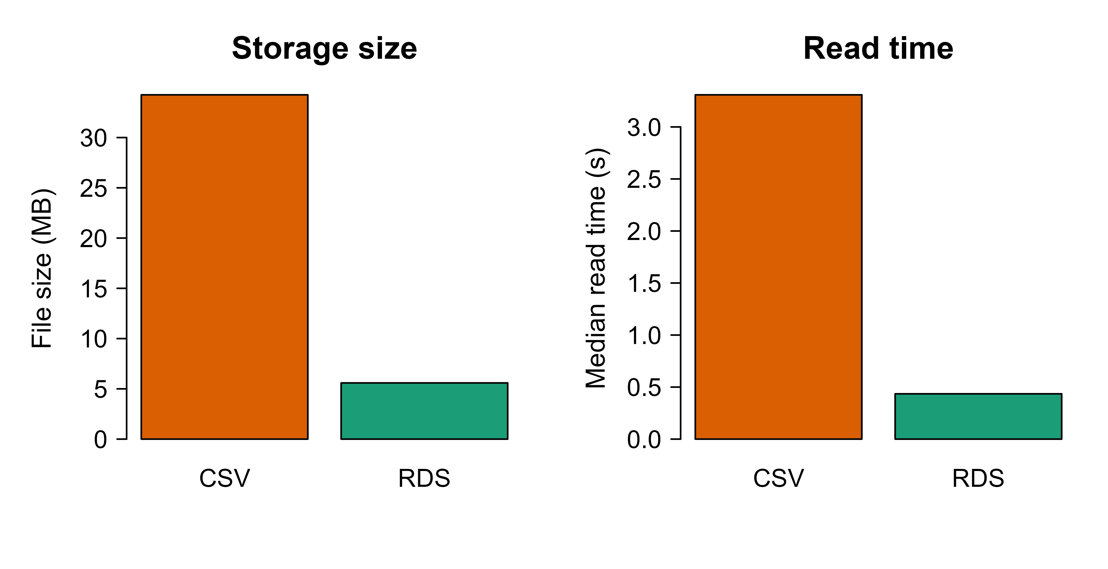
op <- par(mfrow = c(1, 2), mar = c(4, 4, 3, 1))

barplot(results$size_mb, names.arg = results$format,
        col = c("#d95f02", "#1b9e77"),
        ylab = "File size (MB)", main = "Storage size")

barplot(results$read_sec, names.arg = results$format,
        col = c("#d95f02", "#1b9e77"),
        ylab = "Median read time (s)", main = "Read time")

par(op)

Figure 101.1: File size and median read time for the same 1,000,000-row table stored as CSV and as gzip-compressed RDS. Lower is better on both axes.

Figure 101.1 plots the two costs side by side, with file size on the left and median read time on the right. Exact numbers depend on the machine, but the qualitative result is stable: for an R-only workflow, RDS is both smaller and faster than CSV while preserving types exactly. The catch is portability. RDS is readable only by R, so the moment a Python or Spark consumer enters the picture it stops being an option. That is exactly where the columnar formats in the next section earn their keep.

101.8 Columnar formats with arrow (not run here)

The arrow package is not installed in this book’s build environment, so the following chunks are marked eval=FALSE. They are correct, current code you can run after install.packages("arrow"). They show, in code, the columnar advantages this chapter derived in theory: faithful round trips from a stored schema, projection and predicate pushdown, partition pruning, and a fast cross-language handoff.

Tip

Run these yourself after installing arrow, reusing the df from the base R demo above. Comparing the Parquet file size against the CSV and RDS numbers you just measured makes the storage savings concrete.

Writing and reading a single Parquet file, with a choice of codec:

Show code

library(arrow)

# Reuse the same `df` from the base R demo.
parquet_path <- tempfile(fileext = ".parquet")

# zstd gives strong compression; "snappy" or "lz4" are faster, lower ratio.
write_parquet(df, parquet_path, compression = "zstd", compression_level = 5)

# Types are restored from the stored schema: factor stays factor, int stays int.
df_back <- read_parquet(parquet_path)
identical(df, df_back)

file.info(parquet_path)$size / 1024^2   # typically a fraction of the CSV size

Projection and predicate pushdown: read only two columns and only the rows that pass a filter, without loading the whole file into memory. This is the columnar advantage from the I/O ratio derived earlier.

Show code

library(arrow)
library(dplyr)

# open_dataset() builds a lazy query; collect() executes it.
ds <- open_dataset(parquet_path)

result <- ds %>%
  filter(category == "A", value > 110) %>%   # predicate pushdown
  select(id, value) %>%                       # projection pushdown
  collect()

head(result)

Partitioned datasets: write one logical table as many files organized by directory, then query with partition pruning.

Show code

library(arrow)
library(dplyr)

dir_path <- tempfile()
dir.create(dir_path)

# Partition on a low-cardinality column. Avoid partitioning on `id`.
df %>%
  group_by(category) %>%
  write_dataset(path = dir_path, format = "parquet")

# Layout produced: dir_path/category=A/part-0.parquet, category=B/..., etc.
list.files(dir_path, recursive = TRUE)

# A filter on the partition column reads only the matching directory.
open_dataset(dir_path) %>%
  filter(category == "C") %>%
  summarise(mean_value = mean(value)) %>%
  collect()

Feather (Arrow IPC) for a fast handoff to Python, with optional compression:

Show code

library(arrow)

feather_path <- tempfile(fileext = ".feather")

# Uncompressed Feather reads fastest (the file can be memory-mapped);
# use lz4 or zstd when you also want a smaller file.
write_feather(df, feather_path, compression = "lz4")

df_back <- read_feather(feather_path)
identical(df, df_back)

A Python process can read the same file with pandas.read_feather("...") or pyarrow.feather.read_table("...") and get the identical table with types intact, which is the reason these formats dominate cross-language ML pipelines.

JSON, the common interchange format for APIs and nested records, is read row by row and is convenient but verbose and type-loose. In R the tidyverse jsonlite package handles it, and for very large files JSON-lines (one JSON object per line) lets you stream:

Show code

library(jsonlite)

# Pretty JSON for a small object; auto_unbox keeps scalars as scalars.
js <- toJSON(head(df, 3), pretty = TRUE, auto_unbox = TRUE)
cat(js)

# JSON-lines for streaming large data (one record per line).
jsonl_path <- tempfile(fileext = ".jsonl")
stream_out(df, file(jsonl_path))
df_back <- stream_in(file(jsonl_path))

101.9 Practical guidance and pitfalls

The ideas above converge on a short set of decisions. This section collapses them into a when-to-use list and then a list of the mistakes that bite people most often in practice.

The following guidance maps each format to the job it does best:

CSV: small datasets, one-off interchange with tools you do not control, and cases where a human needs to open the file. Do not use it as the storage layer for large or repeatedly-read data, and never rely on it to preserve types.
JSON / JSONL: API payloads, configuration, logs, and genuinely nested or ragged records. Use JSON-lines for large volumes so you can stream and append.
RDS (or qs2 for speed): R objects that only R will consume, especially fitted models, recipes, and workflows from tidymodels (Chapter 90). It is the natural artifact format inside an R project.
Parquet: the default for analysis-ready tabular data of any real size, for feature stores (Chapter 119), and for any dataset shared across R, Python, and Spark. Partition it on date or another low-cardinality filter column.
Feather / Arrow IPC: the fastest option for handing a table between R and Python on the same machine, and for memory-mapping data that does not fit comfortably in RAM. For distributed reads, Parquet is the format Spark expects (Chapter 96).
Avro: row-oriented streaming and message-queue data, and anywhere schema evolution (adding or removing fields over time) is a requirement.

Each of those choices has a matching failure mode. The pitfalls below are the ones that cause silent data corruption or slow pipelines, in rough order of how often they cause real damage:

Trusting CSV type inference. Zip codes and IDs with leading zeros, integers that overflow to doubles, and columns whose first sample rows do not represent later rows all break silently. Declare column types explicitly (readr::read_csv(col_types = ...) or data.table::fread) rather than relying on guesses.
Treating RDS as an interchange format. It is R-only and is tied to R’s serialization version. It is excellent for artifacts inside an R project and unusable for a polyglot team.
The small-files problem. Over-partitioning, or writing one tiny file per batch, produces thousands of small files whose per-file overhead dominates read time. Compact into larger files (roughly 100 MB to 1 GB) and partition only on low-cardinality filter columns.
Wrong codec for the workload. zstd at a high level minimizes storage but costs write CPU; Snappy or LZ4 minimize CPU but store more. Match the codec to whether storage or speed is your bottleneck.
Unsafe deserialization. Reading an RDS or other binary object can execute code embedded by a malicious author. Only deserialize objects from sources you trust.
Floating-point exact-equality expectations. Even faithful columnar round trips can surprise you if you wrote a number in one precision and compare with ==; compare with a tolerance when in doubt.

If you remember one recipe from this chapter, make it this default for a modern R-based ML project: keep raw inputs in whatever form they arrive (often CSV or JSON), convert the cleaned analysis table to partitioned Parquet for repeated reading and cross-language sharing, use Feather for fast same-machine R-to-Python handoffs, and store fitted models and preprocessing objects as RDS. That sequence puts each format where its strengths line up with the cost you are paying at that stage, which is the single principle the rest of the chapter was building toward.

Key idea

Match the format to the stage, not the project. Text in, columnar binary for analysis, language-native for artifacts. Trying to force one format to cover all stages is what creates slow loads and corrupted columns.

101.10 Further reading

Apache Arrow project documentation and the R arrow package documentation (Apache Software Foundation), for Parquet, Feather, and dataset partitioning in R.
Wes McKinney (2017), “Apache Arrow and the Future of Data Frames,” for the motivation behind a shared columnar memory format across languages.
Daniel Abadi, Peter Boncz, and Stavros Harizopoulos (2013), “The Design and Implementation of Modern Column-Oriented Database Systems,” for the theory and engineering of columnar storage and encodings.
Claude Shannon (1948), “A Mathematical Theory of Communication,” for the entropy bound underlying lossless compression.
Hadley Wickham, Mine Cetinkaya-Rundel, and Garrett Grolemund, “R for Data Science” (2nd edition), for practical CSV, JSON, and Parquet handling with the tidyverse and arrow.
The Apache Parquet and Apache Avro format specifications (Apache Software Foundation), for the on-disk layouts, encodings, and schema-evolution rules.

“I/O” is input/output, the work of moving bytes between disk (or network) and memory. It is usually the slowest step in reading data, so a format that reads fewer bytes is faster almost regardless of CPU speed.↩︎
Lossy compression, as in JPEG or MP3, discards detail the human eye or ear is unlikely to notice in exchange for much smaller files. That tradeoff is unacceptable for a data column, where every value must come back exactly, so data formats use only lossless codecs.↩︎
Cardinality is the number of distinct values in a column. Date, region, and category are low to moderate; a user ID or a timestamp to the second is high.↩︎

# Data Formats and Serialization {#sec-data-formats} ```{r} #| include: false source("_common.R") ``` Before a model sees a single row, that data has to be stored somewhere and read back. It is easy to treat that step as plumbing and reach for whatever your last project used, usually a pile of CSV files. The choice of file format, though, is one of the most undervalued decisions in a data science project. It controls how fast you can load a training set, how much disk and cloud storage you pay for, whether a column's type survives a round trip, and whether a downstream engine (R, Python, Spark, a query engine) can read your output at all. Picking well costs nothing extra and can turn a five second load into a quarter second one; picking badly leaves you debugging silently corrupted ID columns at 2 a.m. This chapter builds up the small number of ideas that explain almost every practical difference between formats, then turns those ideas into concrete advice. You will learn what serialization actually is, why some formats store data by row and others by column and why that single choice drives most performance gaps, how compression and schemas work, and how partitioning lets a query skip files it does not need. We then compare the formats you are most likely to meet as a data scientist, analyst, data engineer, or AI/ML engineer working in R: CSV, RDS, JSON, Parquet, Feather/Arrow, and Avro. A runnable demo in base R measures file size and read time for CSV and RDS and produces a figure; code that needs the `arrow` package is shown as `eval=FALSE` but is correct and current, so you can run it after installing that package. ::: {.callout-tip title="When to use this"} Reach for this chapter whenever you are deciding how to store a cleaned dataset, hand a table to a colleague who uses a different language, save a fitted model, or speed up a tuning loop that keeps re-reading the same data. ::: ## Where serialization fits in an ML workflow A typical pipeline moves data through several storage stages: 1. Raw ingestion: data lands from APIs, logs, or exports, often as CSV or JSON because those are what upstream systems emit. 2. Cleaned and typed tables: after parsing and validation, you store an analysis-ready dataset. This is where columnar formats (Parquet, Feather) pay off. 3. Feature stores and training snapshots: large, partitioned datasets read repeatedly during model development and tuning. 4. Model artifacts and intermediate objects: fitted models, preprocessing recipes, and R objects, which is where RDS and `qs2` live. 5. Serving and interchange: predictions and metadata passed to other services, frequently as JSON (see the API chapter, @sec-api). Two costs recur across these stages, and they pull in different directions. The first is read time. During hyperparameter tuning or cross-validation you may read the same training set dozens of times, so a format that reads in 0.2 seconds instead of 5 seconds changes how you work, not just how long you wait. The second is storage cost, which dominates at the feature-store stage, where compression ratios of 5x to 10x translate directly into cloud bills. A recurring theme of this chapter is that no single format wins on both at once, so the right choice depends on which cost you are paying. ::: {.callout-important title="Key idea"} The best format depends on the stage. Human-readable text for ingestion and interchange, columnar binary for analysis-ready tables you read repeatedly, and a language-native format for model artifacts. Few projects should use just one. ::: ### Serialization, formally Serialization is the encoding of an in-memory object into a byte sequence that can be written to disk or sent over a network; deserialization is the inverse. Let $x$ be an in-memory object (a data frame, a model). A format defines an encoder $E: x \mapsto b$ producing bytes $b$, and a decoder $D: b \mapsto x'$. We want the round trip to be faithful, $$ D(E(x)) = x, $$ meaning types, values, and structure are preserved exactly. Many real formats only achieve $D(E(x)) \approx x$: the values look right but the types or precision have quietly shifted. CSV is the classic offender. Because it stores everything as text, a factor comes back as a character column, an integer may come back as a double, dates become strings, and a column of all `NA` loses any sense of its intended type. Formats that carry an explicit schema (Parquet, Avro, Feather) preserve types and give exact round trips for the types they support. ::: {.callout-warning} A "successful" CSV load that returns the right numbers can still be wrong. If a downstream join, model, or comparison depends on a column being an integer or a factor, an approximate round trip is a bug waiting to happen, not a harmless detail. ::: ## Row-oriented versus column-oriented storage The single most useful concept for reasoning about format performance is storage orientation: the order in which values are laid out on disk. A spreadsheet hides this choice behind a grid, but disk is one-dimensional, so the bytes have to come out in some sequence, and there are two natural ways to do it. A row-oriented format stores all fields of record 1, then all fields of record 2, and so on. CSV, JSON-lines, and Avro are row-oriented. To read record $i$ you read a contiguous chunk, which is ideal for transactional workloads that touch whole records and for streaming where records arrive one at a time. A column-oriented (columnar) format stores all values of column 1 together, then all values of column 2, and so on. Parquet and Feather/Arrow are columnar. Analytical workloads usually touch a few columns of many rows (for example, "average revenue by region"), and columnar layout lets you read only the columns you need. ::: {.callout-tip title="Intuition"} Picture a table on a long roll of paper. Row-oriented writing reads it left-to-right, top-to-bottom, so one customer's whole record is together. Columnar writing turns the table on its side, so an entire column sits in one stretch. If you want one customer's details, the first layout is convenient; if you want the average of one column across millions of customers, the second lets you read just that strip and ignore the rest. ::: To make this precise, consider a table with $n$ rows and $p$ columns. Suppose a query reads $k \le p$ columns and applies a filter that keeps a fraction $s \in (0,1]$ of rows (the selectivity). Let $\bar{w}$ be the average bytes per value. A naive row-oriented scan must read essentially the whole file, $$ B_{\text{row}} \approx n \, p \, \bar{w}, $$ because the bytes for the wanted columns are interleaved with everything else. A columnar reader can skip unused columns entirely, and with block-level metadata it can skip blocks that the filter excludes, giving roughly $$ B_{\text{col}} \approx s \, n \, k \, \bar{w}. $$ The ratio is $$ \frac{B_{\text{col}}}{B_{\text{row}}} \approx s \, \frac{k}{p}. $$ For a wide table where you select $k=3$ of $p=100$ columns with $s=0.1$, the columnar reader moves about $0.1 \times 3/100 = 0.003$ of the bytes, a 300x reduction in I/O.^["I/O" is input/output, the work of moving bytes between disk (or network) and memory. It is usually the slowest step in reading data, so a format that reads fewer bytes is faster almost regardless of CPU speed.] This is the mechanism behind the speed of Parquet and Arrow on analytical queries. Skipping unread columns is called *projection pushdown*, and skipping blocks excluded by the filter is called *predicate pushdown*: in both cases the work of selecting is "pushed down" into the reader so it never touches the unwanted bytes. The same accounting explains the flip side: when you must read whole records one at a time, a columnar layout forces you to jump around all $p$ column strips to reassemble each record, so it is a poor fit there. Columnar layout has a second benefit that compounds the first: values in a column share a type and often a narrow range, so they compress far better than a row-interleaved mix of types. That observation leads directly to the next topic. ## Compression Compression replaces a byte sequence with a shorter encoding that decodes back to the original. The formats here all use *lossless* compression, meaning the decoded data equals the original bit for bit, in contrast to the lossy compression used for images or audio.^[Lossy compression, as in JPEG or MP3, discards detail the human eye or ear is unlikely to notice in exchange for much smaller files. That tradeoff is unacceptable for a data column, where every value must come back exactly, so data formats use only lossless codecs.] You might hope to shrink any file arbitrarily, but there is a hard floor: the achievable size is bounded below by the *entropy* of the data, a measure of how unpredictable its values are. If a column's values are drawn from a distribution with probabilities $p_1, \dots, p_m$ over $m$ distinct symbols, Shannon's source coding theorem says the expected bits per value of any lossless code is at least the entropy $$ H = -\sum_{j=1}^{m} p_j \log_2 p_j . $$ A column with low entropy (few distinct values, long runs, or strong autocorrelation) compresses well; a column of unique high-precision floats has entropy near the raw bit width and barely compresses. This is why a `category` column with four levels shrinks dramatically while a column of jittered sensor readings hardly moves. ::: {.callout-tip title="Intuition"} Entropy is the lower bound on "surprise per value." Predictable data (the same code repeated, or numbers that drift slowly) carries little surprise, so a compressor can describe it briefly. Truly random data carries maximum surprise and cannot be shortened, which is also why an already-compressed file does not shrink further when you zip it again. ::: In practice two distinct layers do the work, and it helps to keep them straight. First, encodings exploit structure before any general compressor runs: dictionary encoding replaces repeated strings with small integer codes, run-length encoding collapses repeated values into a value-and-count pair, and delta encoding stores differences between consecutive sorted values rather than the values themselves. Columnar formats apply these per column, which is exactly why grouping like values together helps. Second, codecs are the general-purpose compressors applied on top of the encoded bytes: - Snappy and LZ4: fast, with moderate ratios. Common defaults for Parquet, and the right pick when read or write speed dominates. - Zstandard (zstd): a tunable level that trades CPU for a better ratio, good when storage cost dominates. - gzip: slower, with ratios similar to zstd at low levels; ubiquitous but rarely the best choice for new data. ::: {.callout-tip} A simple rule covers most cases. Use Snappy or LZ4 when speed is the bottleneck, and zstd at a moderate level (say 3 to 9) when storage is the bottleneck. Reserve very high zstd levels for cold, write-once archives where read frequency is low. ::: ## Schemas A schema is the declared structure of a dataset: column names, types, nullability (whether a column may contain missing values), and sometimes nested structure and metadata. The question that separates formats is *when* that structure is decided, and formats fall into three groups along that line. - Schema-on-write (Parquet, Avro, Feather): the schema is stored in the file. A reader knows the exact types without guessing, and a writer can reject data that does not match. This makes round trips faithful and makes data contracts enforceable across teams and languages. - Schema-on-read with inference (CSV): there is no stored schema, so the reader guesses types by sampling rows. Guessing is fragile. A column that is integer for the first 1000 rows but has a decimal at row 50000 may be mis-typed, and an ID like `00123` silently becomes the number `123`. - Self-describing but type-loose (JSON): keys and nesting are explicit per record, but numeric precision and integer-versus-float are not pinned down, and there is no enforced cross-record consistency. ::: {.callout-note} Schema-on-write moves the cost of type decisions to the moment data is written, where the writer has full information, instead of to every future read, where a reader can only guess. That single shift is most of why columnar formats feel reliable in pipelines that run unattended. ::: Avro deserves a note here, because it does not fit the usual pairing of "columnar and strict" versus "row-oriented and loose." It is row-oriented yet schema-on-write, and it adds schema evolution: readers and writers can use different but compatible schema versions, so you can add a field with a default or drop an optional field without breaking data already written under the old schema. That property is what makes Avro a common choice for long-lived streaming and message-queue data, where the record shape changes over months but old records must still be readable. ## Partitioning Predicate pushdown lets a reader skip blocks *within* a file. Partitioning takes the same idea up a level and lets it skip whole files. It splits one logical dataset into many files organized by the values of one or more columns, usually encoded in the directory path, for example `year=2025/month=06/part-0.parquet`. A query that filters on a partition column reads only the matching directories, a technique called *partition pruning*. If a dataset is partitioned on a column with $d$ distinct values and a query selects one of them, the reader touches about $1/d$ of the files before any within-file filtering even begins. The trick is choosing the partition column well. Partitioning works best on low-to-moderate cardinality columns^[*Cardinality* is the number of distinct values in a column. Date, region, and category are low to moderate; a user ID or a timestamp to the second is high.] that appear often in filters, such as date, region, or category. Partitioning on a high-cardinality column like a user ID creates millions of tiny files and hurts performance badly, an anti-pattern known as the *small-files problem*: the per-file bookkeeping (open, read metadata, close) swamps the actual data reading. ::: {.callout-warning} More partitions is not better. Aim for files in the range of roughly 100 MB to 1 GB each. If partitioning would push file sizes far below that, the column has too high a cardinality to partition on. ::: ## The formats at a glance With orientation, compression, schemas, and partitioning in hand, the individual formats become easy to read off as combinations of those choices. @tbl-data-formats-summary summarizes them; treat it as a lookup card to scan, and read the clarifications underneath for the two formats most often misunderstood. | Format | Orientation | Schema | Typical compression | Cross-language | Best for | |---|---|---|---|---|---| | CSV | Row (text) | None (inferred) | None by default (can gzip) | Yes (universal) | Interchange, small data, human inspection | | JSON / JSONL | Row (text) | Self-describing, loose | None by default | Yes (universal) | APIs, nested records, config, logs | | RDS | R object | Implicit (R types) | gzip (default) | No (R only) | R objects, models, recipes | | Parquet | Column | Stored | Snappy / zstd / gzip | Yes (Arrow, Spark, etc.) | Large analytical tables, feature stores | | Feather / Arrow IPC | Column | Stored | LZ4 / zstd / none | Yes (Arrow ecosystem) | Fast R/Python handoff, memory mapping | | Avro | Row | Stored, evolvable | Snappy / deflate | Yes | Streaming, message queues, evolving records | : Comparison of the common data formats by storage orientation, schema handling, typical compression, cross-language support, and the workload each is best suited to. {#tbl-data-formats-summary} A few clarifications. "Feather" version 2 is the on-disk form of the Arrow IPC format; it is columnar and uncompressed-by-default reads are very fast because the on-disk layout matches the in-memory layout, allowing memory mapping. RDS is R's native serialization: it preserves any R object exactly (factors, attributes, S4 classes, fitted models) but only R can read it, so it is the right tool for model artifacts and the wrong tool for tables you want to share with a Python team. ## Runnable demo: CSV versus RDS in base R Enough theory; let us measure it. The following demonstration uses only base R, so it runs anywhere without extra packages. It builds a moderately sized data frame with mixed column types, writes it as CSV and as RDS (gzip-compressed, which is the default), and measures file size and read time on a one-million-row table. It then shows the type-fidelity problem directly: a factor survives the RDS round trip but not the CSV one. Finally it plots the comparison so the size and speed gaps are visible at a glance. ```{r data-formats-setup, eval=TRUE} set.seed(1301) n <- 1000000 df <- data.frame( id = 1:n, category = factor(sample(c("A", "B", "C", "D"), n, replace = TRUE)), count = sample(0:50L, n, replace = TRUE), # integer value = round(rnorm(n, mean = 100, sd = 15), 4), # double flag = sample(c(TRUE, FALSE), n, replace = TRUE), # logical label = sample(c("low", "medium", "high"), n, replace = TRUE), stringsAsFactors = FALSE ) str(df) ``` ```{r data-formats-write-read, eval=TRUE} csv_path <- tempfile(fileext = ".csv") rds_path <- tempfile(fileext = ".rds") # A small high-resolution timer (Sys.time has sub-millisecond resolution). # It captures the unevaluated call and re-runs it once per repetition. timeit <- function(call) { call <- substitute(call) t0 <- Sys.time() eval(call, envir = parent.frame()) as.numeric(difftime(Sys.time(), t0, units = "secs")) } # Write timing csv_write <- timeit(write.csv(df, csv_path, row.names = FALSE)) rds_write <- timeit(saveRDS(df, rds_path)) # gzip by default # File sizes in megabytes mb <- function(path) file.info(path)$size / 1024^2 csv_size <- mb(csv_path) rds_size <- mb(rds_path) # Read timing: re-run the read several times, take the median to reduce noise. median_read_time <- function(call, reps = 5) { call <- substitute(call) times <- numeric(reps) for (i in seq_len(reps)) { t0 <- Sys.time() eval(call, envir = parent.frame()) times[i] <- as.numeric(difftime(Sys.time(), t0, units = "secs")) } median(times) } csv_read <- median_read_time(read.csv(csv_path, stringsAsFactors = FALSE)) rds_read <- median_read_time(readRDS(rds_path)) results <- data.frame( format = c("CSV", "RDS"), size_mb = c(csv_size, rds_size), write_sec = c(csv_write, rds_write), read_sec = c(csv_read, rds_read), row.names = NULL ) print(results, digits = 3) ``` The RDS file is smaller because it is gzip-compressed and stores values in a compact binary form rather than as text, and it reads faster because no text parsing or type inference is needed. On a typical machine the RDS file is several times smaller and reads several times faster, which is the whole point: for repeated reads inside a tuning loop, those factors multiply. Speed and size are only half the story. A faster format is no use if it hands back the wrong types. The fidelity check below compares the column types of the original data frame against what each format gives back. ```{r data-formats-fidelity, eval=TRUE} csv_back <- read.csv(csv_path, stringsAsFactors = FALSE) rds_back <- readRDS(rds_path) types <- function(d) vapply(d, function(col) class(col)[1], character(1)) fidelity <- data.frame( column = names(df), original = types(df), csv = types(csv_back)[names(df)], rds = types(rds_back)[names(df)], row.names = NULL ) print(fidelity) # Exact round trip? cat("RDS identical to original:", identical(df, rds_back), "\n") cat("CSV identical to original:", identical(df, csv_back), "\n") ``` The RDS round trip is exact: `identical()` returns `TRUE`. The CSV round trip is not, because CSV changes types. The `category` factor comes back as a plain character column, since text on disk carries no notion of factor levels. This is not a bug in R; it is the direct consequence of CSV storing only text with no schema. Whether a numeric column survives is a matter of luck: an integer column like `count` happens to re-infer as integer here because every value is whole, but a column whose first sampled rows look integer and whose later rows contain a decimal would be silently re-typed. ::: {.callout-warning} Do not read CSV fidelity off this one example and conclude integers are safe. The factor loss is guaranteed; numeric type survival is incidental and depends entirely on the data sampled during inference. Treat any CSV round trip as approximate unless you declare column types explicitly. ::: ### Figure: size and read-time comparison ```{r fig-data-formats-figure, eval=TRUE, fig.width=7, fig.height=3.6, fig.cap="File size and median read time for the same 1,000,000-row table stored as CSV and as gzip-compressed RDS. Lower is better on both axes."} op <- par(mfrow = c(1, 2), mar = c(4, 4, 3, 1)) barplot(results$size_mb, names.arg = results$format, col = c("#d95f02", "#1b9e77"), ylab = "File size (MB)", main = "Storage size") barplot(results$read_sec, names.arg = results$format, col = c("#d95f02", "#1b9e77"), ylab = "Median read time (s)", main = "Read time") par(op) ``` @fig-data-formats-figure plots the two costs side by side, with file size on the left and median read time on the right. Exact numbers depend on the machine, but the qualitative result is stable: for an R-only workflow, RDS is both smaller and faster than CSV while preserving types exactly. The catch is portability. RDS is readable only by R, so the moment a Python or Spark consumer enters the picture it stops being an option. That is exactly where the columnar formats in the next section earn their keep. ## Columnar formats with arrow (not run here) The `arrow` package is not installed in this book's build environment, so the following chunks are marked `eval=FALSE`. They are correct, current code you can run after `install.packages("arrow")`. They show, in code, the columnar advantages this chapter derived in theory: faithful round trips from a stored schema, projection and predicate pushdown, partition pruning, and a fast cross-language handoff. ::: {.callout-tip} Run these yourself after installing `arrow`, reusing the `df` from the base R demo above. Comparing the Parquet file size against the CSV and RDS numbers you just measured makes the storage savings concrete. ::: Writing and reading a single Parquet file, with a choice of codec: ```{r arrow-parquet-basic, eval=FALSE} library(arrow) # Reuse the same `df` from the base R demo. parquet_path <- tempfile(fileext = ".parquet") # zstd gives strong compression; "snappy" or "lz4" are faster, lower ratio. write_parquet(df, parquet_path, compression = "zstd", compression_level = 5) # Types are restored from the stored schema: factor stays factor, int stays int. df_back <- read_parquet(parquet_path) identical(df, df_back) file.info(parquet_path)$size / 1024^2 # typically a fraction of the CSV size ``` Projection and predicate pushdown: read only two columns and only the rows that pass a filter, without loading the whole file into memory. This is the columnar advantage from the I/O ratio derived earlier. ```{r arrow-pushdown, eval=FALSE} library(arrow) library(dplyr) # open_dataset() builds a lazy query; collect() executes it. ds <- open_dataset(parquet_path) result <- ds %>% filter(category == "A", value > 110) %>% # predicate pushdown select(id, value) %>% # projection pushdown collect() head(result) ``` Partitioned datasets: write one logical table as many files organized by directory, then query with partition pruning. ```{r arrow-partition, eval=FALSE} library(arrow) library(dplyr) dir_path <- tempfile() dir.create(dir_path) # Partition on a low-cardinality column. Avoid partitioning on `id`. df %>% group_by(category) %>% write_dataset(path = dir_path, format = "parquet") # Layout produced: dir_path/category=A/part-0.parquet, category=B/..., etc. list.files(dir_path, recursive = TRUE) # A filter on the partition column reads only the matching directory. open_dataset(dir_path) %>% filter(category == "C") %>% summarise(mean_value = mean(value)) %>% collect() ``` Feather (Arrow IPC) for a fast handoff to Python, with optional compression: ```{r arrow-feather, eval=FALSE} library(arrow) feather_path <- tempfile(fileext = ".feather") # Uncompressed Feather reads fastest (the file can be memory-mapped); # use lz4 or zstd when you also want a smaller file. write_feather(df, feather_path, compression = "lz4") df_back <- read_feather(feather_path) identical(df, df_back) ``` A Python process can read the same file with `pandas.read_feather("...")` or `pyarrow.feather.read_table("...")` and get the identical table with types intact, which is the reason these formats dominate cross-language ML pipelines. JSON, the common interchange format for APIs and nested records, is read row by row and is convenient but verbose and type-loose. In R the tidyverse `jsonlite` package handles it, and for very large files JSON-lines (one JSON object per line) lets you stream: ```{r json-demo, eval=FALSE} library(jsonlite) # Pretty JSON for a small object; auto_unbox keeps scalars as scalars. js <- toJSON(head(df, 3), pretty = TRUE, auto_unbox = TRUE) cat(js) # JSON-lines for streaming large data (one record per line). jsonl_path <- tempfile(fileext = ".jsonl") stream_out(df, file(jsonl_path)) df_back <- stream_in(file(jsonl_path)) ``` ## Practical guidance and pitfalls The ideas above converge on a short set of decisions. This section collapses them into a when-to-use list and then a list of the mistakes that bite people most often in practice. The following guidance maps each format to the job it does best: - CSV: small datasets, one-off interchange with tools you do not control, and cases where a human needs to open the file. Do not use it as the storage layer for large or repeatedly-read data, and never rely on it to preserve types. - JSON / JSONL: API payloads, configuration, logs, and genuinely nested or ragged records. Use JSON-lines for large volumes so you can stream and append. - RDS (or `qs2` for speed): R objects that only R will consume, especially fitted models, `recipes`, and `workflows` from tidymodels (@sec-tidymodels-framework). It is the natural artifact format inside an R project. - Parquet: the default for analysis-ready tabular data of any real size, for feature stores (@sec-feature-stores), and for any dataset shared across R, Python, and Spark. Partition it on date or another low-cardinality filter column. - Feather / Arrow IPC: the fastest option for handing a table between R and Python on the same machine, and for memory-mapping data that does not fit comfortably in RAM. For distributed reads, Parquet is the format Spark expects (@sec-spark-sparklyr). - Avro: row-oriented streaming and message-queue data, and anywhere schema evolution (adding or removing fields over time) is a requirement. Each of those choices has a matching failure mode. The pitfalls below are the ones that cause silent data corruption or slow pipelines, in rough order of how often they cause real damage: - Trusting CSV type inference. Zip codes and IDs with leading zeros, integers that overflow to doubles, and columns whose first sample rows do not represent later rows all break silently. Declare column types explicitly (`readr::read_csv(col_types = ...)` or `data.table::fread`) rather than relying on guesses. - Treating RDS as an interchange format. It is R-only and is tied to R's serialization version. It is excellent for artifacts inside an R project and unusable for a polyglot team. - The small-files problem. Over-partitioning, or writing one tiny file per batch, produces thousands of small files whose per-file overhead dominates read time. Compact into larger files (roughly 100 MB to 1 GB) and partition only on low-cardinality filter columns. - Wrong codec for the workload. zstd at a high level minimizes storage but costs write CPU; Snappy or LZ4 minimize CPU but store more. Match the codec to whether storage or speed is your bottleneck. - Unsafe deserialization. Reading an RDS or other binary object can execute code embedded by a malicious author. Only deserialize objects from sources you trust. - Floating-point exact-equality expectations. Even faithful columnar round trips can surprise you if you wrote a number in one precision and compare with `==`; compare with a tolerance when in doubt. If you remember one recipe from this chapter, make it this default for a modern R-based ML project: keep raw inputs in whatever form they arrive (often CSV or JSON), convert the cleaned analysis table to partitioned Parquet for repeated reading and cross-language sharing, use Feather for fast same-machine R-to-Python handoffs, and store fitted models and preprocessing objects as RDS. That sequence puts each format where its strengths line up with the cost you are paying at that stage, which is the single principle the rest of the chapter was building toward. ::: {.callout-important title="Key idea"} Match the format to the stage, not the project. Text in, columnar binary for analysis, language-native for artifacts. Trying to force one format to cover all stages is what creates slow loads and corrupted columns. ::: ## Further reading - Apache Arrow project documentation and the R `arrow` package documentation (Apache Software Foundation), for Parquet, Feather, and dataset partitioning in R. - Wes McKinney (2017), "Apache Arrow and the Future of Data Frames," for the motivation behind a shared columnar memory format across languages. - Daniel Abadi, Peter Boncz, and Stavros Harizopoulos (2013), "The Design and Implementation of Modern Column-Oriented Database Systems," for the theory and engineering of columnar storage and encodings. - Claude Shannon (1948), "A Mathematical Theory of Communication," for the entropy bound underlying lossless compression. - Hadley Wickham, Mine Cetinkaya-Rundel, and Garrett Grolemund, "R for Data Science" (2nd edition), for practical CSV, JSON, and Parquet handling with the tidyverse and arrow. - The Apache Parquet and Apache Avro format specifications (Apache Software Foundation), for the on-disk layouts, encodings, and schema-evolution rules.