Self-supervised learning trains a model to predict some part of its input from another part, using the structure of unlabeled data as the supervision signal. There are no human labels. The labels are constructed automatically from the data itself, which is why the approach scales to the large unlabeled corpora that data teams already hold. The output of self-supervised training is not a classifier or a regressor. It is a learned representation: a function that maps raw inputs to vectors that make downstream tasks easier. Once a good representation exists, a small labeled dataset and a simple model (often a linear layer) are enough to solve the task you actually care about.
This chapter covers the main families of self-supervised methods used in practice: pretext tasks, contrastive learning with the InfoNCE objective, the SimCLR and MoCo training recipes, the non-contrastive BYOL approach, and masked modeling as used by BERT and masked autoencoders. The recurring question is why a representation learned without labels transfers to tasks that have labels. We work through the InfoNCE loss in detail and give a runnable base-R demonstration that shows exactly how positive and negative pairs move the loss.
Key idea
Self-supervised learning does not solve your task directly. It learns a representation, a reusable map from raw input to a vector, and a small labeled step turns that representation into the model you need. Keep the two stages separate in your mind: learning the map, then using the map.
Note
“Self-supervised” and “unsupervised” are often used loosely, but they are not the same. Unsupervised learning (clustering, covered in Chapter 23, and density estimation, covered in Chapter 32) has no target at all. Self-supervised learning invents a target from the input, so the machinery of supervised training (a loss, gradients, a prediction) still applies; only the labels are free.
49.1 Where This Fits in a Modern Workflow
Most teams sit on far more unlabeled data than labeled data. Logs, images, documents, sensor traces, and user events accumulate continuously, while labeling is slow and expensive. Self-supervised learning turns the cheap, abundant resource into a pretrained representation, and reserves the scarce labels for a short fine-tuning step.
A typical pipeline has three stages.
Pretrain. Train an encoder \(f_\theta\) on unlabeled data with a self-supervised objective. This is the expensive step and it is done once, often by a separate team or downloaded as a public checkpoint.
Transfer. Freeze or lightly fine-tune \(f_\theta\) and attach a small task head. With frozen features this is called linear probing: fit a linear model on top of \(f_\theta(x)\). The quality of the representation is often reported as the accuracy of this linear probe.
Fine-tune. If labels are plentiful enough, unfreeze the encoder and train the whole stack at a low learning rate so the representation adapts to the task.
Tip
Most practitioners never run stage 1. The expensive pretraining is done once by a well-resourced lab and released as a public checkpoint, so your day-to-day work is stages 2 and 3 on top of someone else’s encoder. Knowing how the encoder was trained still matters, because it tells you what the representation is invariant to and therefore what it will quietly ignore.
This is the same shape as the transfer-learning workflow (Chapter 54) behind BERT (Chapter 39) for text and pretrained vision backbones for images. The difference from supervised pretraining is only the source of the training signal: the structure of the data instead of external labels.
49.2 Pretext Tasks
The earliest self-supervised methods invent a pretext task: a supervised problem whose labels are free because they come from the data. Solving the pretext task well is not the goal. The goal is that the features the model builds while solving it are useful for real tasks.
Examples that shaped the field:
Context prediction. Given two image patches, predict their relative spatial arrangement. To answer, the model must recognize object parts and their layout.
Rotation prediction. Rotate an image by \(0, 90, 180,\) or \(270\) degrees and predict the angle. Getting this right requires knowing the canonical orientation of objects.
Colorization. Remove color and predict it back. The model has to associate textures and shapes with plausible colors.
Jigsaw puzzles. Shuffle image tiles and predict the permutation.
The weakness of hand-designed pretext tasks is that the model can exploit shortcuts.1 A rotation predictor might key on watermarks or sky-at-top cues rather than object structure. Contrastive and masked methods, covered next, are more robust because the supervision is harder to game.
Intuition
A pretext task is a teacher who sets a puzzle hoping the student learns something general while solving it. The risk is the same as in a classroom: the student may find a trick that aces the puzzle and teaches nothing. The methods that follow design puzzles where the only winning strategy is to actually understand the content.
49.3 Contrastive Learning and the InfoNCE Objective
Contrastive learning replaces a single hand-built pretext task with a general principle: representations of two views of the same item should be close, and representations of different items should be far apart. “Close” and “far” are measured by a similarity in the representation space.
49.3.1 Views and the Similarity
Start with an input \(x\) and apply two random transformations to get two views, \(\tilde x\) and \(\tilde x^{+}\). For images the transformations are crops, color shifts, and blurs. For text they can be token masking or dropout. The pair \((\tilde x, \tilde x^{+})\) is a positive pair: two views of the same underlying item. Views of other items in the batch are negatives.
An encoder \(f_\theta\) maps a view to a vector, usually followed by a small projection head and an \(\ell_2\) normalization so that every representation lies on the unit sphere.2 Write the normalized representations as \(z = f_\theta(\tilde x)\) and \(z^{+} = f_\theta(\tilde x^{+})\) with \(\lVert z \rVert = 1\). Similarity is the dot product (cosine similarity on the unit sphere),
\[
\operatorname{sim}(u, v) = u^\top v .
\]
49.3.2 The Loss
Consider a query \(z\) with one positive \(z^{+}\) and a set of negatives \(\{z^{-}_1, \dots, z^{-}_K\}\). The InfoNCE loss, also called the normalized temperature-scaled cross-entropy loss, is
The temperature \(\tau > 0\) scales the similarities before the softmax. Read the fraction as a classification problem: among the \(K+1\) candidates (one positive and \(K\) negatives), which one is the true match for \(z\)? The loss is the cross-entropy of a softmax classifier that has to pick the positive. Minimizing it pushes \(z^\top z^{+}\) up and pushes each \(z^\top z^{-}_k\) down.
Intuition
Picture a lineup. The query \(z\) is shown a row of candidates, exactly one of which is its partner view. InfoNCE rewards the encoder for confidently fingering the right partner. To win this game across many lineups, the encoder has no choice but to place each item’s two views near each other and away from everyone else.
The temperature controls how sharply the loss focuses on the hardest negatives. Small \(\tau\) makes the softmax sharp, so negatives with high similarity to the query dominate the gradient. Large \(\tau\) flattens the distribution and treats all negatives more equally. In practice \(\tau\) is a sensitive hyperparameter, often near \(0.1\).
49.3.3 Why It Learns a Useful Representation
InfoNCE has an information-theoretic reading. Let \(z\) and \(z^{+}\) be representations of two views that share the same latent content. Minimizing the expected InfoNCE loss with \(K\) negatives maximizes a lower bound on the mutual information between the two views,
The bound says the loss is a budget: pushing \(\mathcal{L}_{\text{InfoNCE}}\) down raises the guaranteed floor on the shared information \(I(z; z^{+})\), and more negatives (\(K\) large) raise the ceiling \(\log(K+1)\) that the floor can reach.3 So driving the loss down forces the representation to keep whatever information is shared across views and discard what is not. The transformations are chosen so that the shared content is the semantic identity of the item (the object in an image, the meaning of a sentence) and the discarded part is nuisance variation (crop position, color jitter, exact wording). That is the mechanism behind transfer: the representation retains task-relevant structure because that structure is what survives across views, and it drops the nuisance factors that a downstream task would also want to ignore.
A second, more geometric view comes from decomposing the loss. Writing it out, InfoNCE pushes for alignment (positives close) and uniformity (representations spread over the sphere so they stay distinguishable). The negatives supply the uniformity pressure. Without them, the encoder could map every input to the same point, drive all positive similarities to one, and make the loss small while learning nothing. This failure is called representation collapse, and avoiding it is the central design problem for the methods below.
49.3.4 Formal Setup and the Loss as a Conditional Likelihood
To make the objective precise, fix the data-generating process. Let \(x\) be drawn from the data distribution \(p(x)\), and let a stochastic augmentation \(t \sim \mathcal{T}\) produce a view \(\tilde x = t(x)\). Two independent draws \(t, t' \sim \mathcal{T}\) give the positive pair \((\tilde x, \tilde x^{+})\). The encoder \(g_\theta\) (encoder plus projection head) maps a view to \(\mathbb{R}^m\), and we normalize \(z = g_\theta(\tilde x)/\lVert g_\theta(\tilde x)\rVert\) so that \(z \in \mathcal{S}^{m-1}\), the unit sphere. The temperature \(\tau>0\) is fixed.
InfoNCE is exactly the negative log-likelihood of a softmax classifier whose job is to pick the positive out of a candidate set of size \(K+1\). Index the candidates \(0,1,\dots,K\) with candidate \(0\) the positive. Define the categorical model
The loss \(\ell(z) = -\log p_\theta(\text{match}=0\mid \cdot)\) in Equation 49.1 reproduces the InfoNCE loss above. Reading it as a \((K+1)\)-way classification makes the connection to cross-entropy literal: the network outputs logits \(z^\top z_j/\tau\) and the free label is “the positive sits in slot \(0\).”
49.3.5 Derivation: InfoNCE as a Mutual-Information Lower Bound
We now derive the bound \(I(z;z^{+}) \ge \log(K+1) - \mathcal{L}_{\text{InfoNCE}}\) stated above, following the contrastive predictive coding argument. The key is that the optimal critic recovers a density ratio.
Consider one positive sample drawn from the joint \(p(z, z^{+})\) and \(K\) negatives drawn independently from the marginal \(p(z^{+})\). Collect the \(K+1\) candidates in \(Z=\{z_0,\dots,z_K\}\), with the positive placed uniformly at a random slot. The posterior probability that slot \(i\) holds the positive, given \(z\) and \(Z\), is by Bayes’ rule
where the second equality divides numerator and denominator by \(\prod_{j} p(z_j)\). The Bayes-optimal classifier therefore scores each candidate by the density ratio \(r(z_i, z) = p(z_i\mid z)/p(z_i) = p(z, z_i)/(p(z)p(z_i))\). Comparing with Equation 49.1, the softmax classifier is Bayes-optimal exactly when the learned similarity matches the log density ratio up to a \(z\)-dependent constant,
The \(K\) negative terms are i.i.d. draws from the marginal, so \(\mathbb{E}_{z_k}\big[p(z_k\mid z)/p(z_k)\big]=\int p(z_k\mid z)\,dz_k = 1\). By the law of large numbers the inner sum concentrates on its mean, \(\sum_{k=1}^{K} p(z_k\mid z)/p(z_k) \approx K\,\mathbb{E}_{z_k}\big[p(z_k\mid z)/p(z_k)\big] = K\) (this concentration approximation, not Jensen, is the step that makes the argument non-rigorous), which yields
Two consequences follow immediately from Equation 49.4. First, the bound is loose by at most \(\log(K+1)\), so it can certify at most \(\log(K+1)\) nats of mutual information; this is the precise sense in which more negatives raise the ceiling. Second, if the true \(I(z;z^{+})\) exceeds \(\log(K+1)\), the loss cannot be driven to zero no matter how good the encoder, which is why InfoNCE saturates and why large \(K\) matters for high-information modalities.
The bias of the bound
Equation 49.4 is a lower bound on \(I(z;z^{+})\), so minimizing the loss is a surrogate, not a direct maximization of mutual information. The slack \(\log(K+1)-\mathcal{L}\) is what you actually control. Estimators of mutual information based on this bound are known to have variance and bias that grow with the true information, so InfoNCE is best read as a representation objective whose MI interpretation is a guide, not a guarantee.
49.3.6 Derivation: The Alignment and Uniformity Decomposition
The geometric picture can be made exact in the limit of infinitely many negatives. Write the per-sample loss with negatives drawn from the marginal \(p_z\) over the sphere,
Take expectations and let \(K\to\infty\). The first term becomes the negative expected positive similarity, and by the law of large numbers the sum inside the log concentrates on \(K\,\mathbb{E}_{z^-}\exp(z^\top z^-/\tau)\). Dropping the additive \(\log K\) constant, the asymptotic objective splits into two pieces,
The alignment term is minimized when positive pairs are identical on the sphere. The uniformity term in Equation 49.5 is, up to constants, the logarithm of the Gaussian-kernel potential \(\mathbb{E}\,e^{-\lVert z - z^{-}\rVert^2/(2\tau)\cdot c}\) (using \(\lVert z-z^-\rVert^2 = 2-2z^\top z^-\) on the unit sphere). Minimizing it spreads the representations as uniformly as possible over \(\mathcal{S}^{m-1}\); its global minimizer is the uniform distribution on the sphere. This is the formal statement that negatives supply uniformity pressure and positives supply alignment pressure, and it explains collapse directly: with no negatives the uniformity term vanishes and the alignment term alone is minimized by the constant map.
49.3.7 Derivation: The InfoNCE Gradient and Hard-Negative Weighting
To see why small temperature emphasizes hard negatives, differentiate. With \(s_j = z^\top z_j/\tau\) and softmax weights \(p_j = e^{s_j}/\sum_k e^{s_k}\) over the candidates (positive at slot \(0\)), the loss is \(\ell = -s_0 + \log\sum_j e^{s_j}\), so
The gradient pulls \(z\) toward the positive (the \((p_0-1)z_0\) term, since \(p_0-1<0\)) and pushes it away from each negative with weight \(p_k\). Because \(p_k \propto e^{z^\top z_k/\tau}\), a hard negative (large \(z^\top z_k\)) receives an exponentially larger repulsion weight as \(\tau\to 0\). Thus small \(\tau\) concentrates the gradient on the few hardest negatives, sharpening the decision boundary but increasing variance; large \(\tau\) averages over all negatives, which is gentler but blurs the contrast. This is the analytic content behind the earlier remark that \(\tau\) trades hard-negative focus against stability.
Warning
Collapse is the recurring villain of self-supervised learning. Watch for it whenever a method has alignment pressure but weak or no uniformity pressure. The two terms are in tension: alignment alone wants to crush everything together, uniformity alone wants to scatter it, and a good representation is the balance between them.
49.4 SimCLR and MoCo: Two Ways to Get Negatives
InfoNCE needs many negatives to give a strong uniformity signal and a tight mutual-information bound. The two influential recipes differ mainly in where the negatives come from.
SimCLR uses the other items in the current minibatch as negatives. For a batch of \(N\) items it makes two views of each, giving \(2N\) views; for any view its positive is the other view of the same item and the remaining \(2N-2\) views are negatives. This is simple and has no extra moving parts, but it needs large batches (thousands) to have enough negatives, which costs memory.
MoCo (Momentum Contrast) decouples the number of negatives from the batch size. It keeps a queue of representations from recent batches to act as negatives, so the effective negative set is large even with a modest batch. The negatives are encoded by a second momentum encoder whose weights are an exponential moving average of the main encoder,
\[
\theta_{\text{key}} \leftarrow m \, \theta_{\text{key}} + (1 - m)\, \theta_{\text{query}}, \qquad m \in [0, 1) \text{ close to } 1 .
\]
The slow-moving key encoder keeps the queued representations consistent over time, which matters because they were computed by slightly older weights.
49.4.1 SimCLR: the NT-Xent Loss Made Precise
In a SimCLR batch of \(N\) items, augmentation produces \(2N\) views indexed \(i=1,\dots,2N\), where view \(i\) and its partner \(j(i)\) are the two views of the same item. With normalized projections \(z_i\) and similarity \(s_{ik}=z_i^\top z_k/\tau\), the per-view NT-Xent loss excludes self-comparison,
Each view in Equation 49.7 sees \(K = 2N-2\) negatives, so the effective negative count is tied directly to batch size; this is why SimCLR needs batches in the thousands to make the \(\log(K+1)\) ceiling in Equation 49.4 useful. The cost is the \((2N)\times(2N)\) similarity matrix, which is \(O(N^2 m)\) to form and \(O(N^2)\) memory, dominating large-batch training. The loss is symmetric in the two views because every view serves as a query.
49.4.2 MoCo as a Dictionary Lookup and the Role of Momentum
MoCo reframes contrastive learning as lookup against a dictionary. The query \(q=g_{\theta_q}(\tilde x)\) is matched against keys \(\{k_0,k_1,\dots\}\), where \(k_0\) is the positive key and the rest come from a FIFO queue of size \(K\) encoded by the momentum encoder. The loss is the single-query InfoNCE,
Decoupling \(K\) from batch size is the central trick: the queue accumulates negatives across many past steps, so \(K\) can be tens of thousands with a batch of a few hundred. The momentum update \(\theta_{\text{key}} \leftarrow m\,\theta_{\text{key}} + (1-m)\,\theta_{\text{query}}\) is what makes this safe. If the key encoder were updated by gradient like the query encoder, the queued keys would be stale: representations computed several hundred steps ago by rapidly changing weights would no longer be comparable to current queries, and training would diverge. The slow update keeps the key encoder approximately constant over the lifetime of the queue. Concretely, a key enters the queue and is evicted after \(K/\,(\text{batch size})\) steps; over that span \(\theta_{\text{key}}\) moves by roughly a factor \(1-m^{K/\text{batch}}\), so \(m\) near \(0.999\) keeps the dictionary consistent. Empirically large \(m\) (0.99 to 0.999) is essential; \(m=0\) (no momentum, key encoder equals query encoder) collapses performance.
When to use this
Choose SimCLR when you can afford large batches and want the simplest pipeline. Choose MoCo when GPU memory caps your batch size but you still want many negatives; its queue lets a small batch see thousands of negatives accumulated over recent steps.
49.5 BYOL: Contrastive Without Negatives
BYOL (Bootstrap Your Own Latent) removes negatives entirely and still avoids collapse. At first glance this should be impossible: with no negatives, what stops the encoder from mapping everything to one point? That puzzle is exactly what makes BYOL interesting. It uses two networks: an online network and a target network. The online network sees one view and is asked to predict the target network’s representation of the other view. The target network is again an exponential moving average of the online network and is not trained by gradients.4
The objective is a regression toward the target representation, typically the squared error between \(\ell_2\)-normalized vectors,
where \(q\) is a predictor on the online side and the bar denotes normalization. Two ingredients keep the trivial constant solution away: the extra predictor \(q\) on only the online side breaks the symmetry between the two branches, and the stop-gradient on the target branch means the target does not chase the online network. The result is competitive with contrastive methods without ever forming a negative pair, which removes the large-batch and queue machinery. A related method, SimSiam, shows that even the moving-average target can be dropped if the stop-gradient and predictor are kept.
49.5.1 Why BYOL Does Not Collapse: the Stop-Gradient Argument
It is worth being precise about the puzzle, because the resolution is subtle and the naive analysis predicts collapse. Expand the BYOL objective with online encoder \(f_\theta\), predictor \(q_\theta\), target encoder \(f_\xi\), and stop-gradient \(\operatorname{sg}\),
The constant map (\(f\) outputs a fixed vector) is a global minimizer with loss zero, so nothing in the objective forbids collapse. SimSiam analyzes why gradient descent nonetheless avoids it by reading the procedure as alternating optimization of an auxiliary problem. Introduce a per-image latent target \(\eta_x\) and the surrogate
Holding \(\theta\) fixed, the optimal \(\eta_x\) is the expectation \(\mathbb{E}_{t}\,f_\theta(t(x))\), which is what the stop-gradient branch (with its slow target) approximates. Holding \(\eta\) fixed, a gradient step updates \(\theta\). The stop-gradient is exactly what makes this an alternating two-variable minimization rather than a single joint descent that would collapse. The predictor \(q_\theta\) is the second guard: because the optimal predictor outputs the conditional mean \(q^\star(f_\theta(\tilde x)) = \mathbb{E}_{\tilde x^{+}}[\,\overline{f_\xi(\tilde x^{+})}\mid f_\theta(\tilde x)\,]\), it absorbs the augmentation-induced variance and removes the gradient pressure that would otherwise shrink all representations to a point. Remove either ingredient and BYOL collapses, which the SimSiam ablations confirm. The exponential-moving-average target adds stability but is not strictly necessary once stop-gradient and predictor are present.
Connection to contrastive methods
BYOL has no explicit uniformity term, so it cannot be analyzed through Equation 49.5. Its anti-collapse mechanism is dynamical (a property of the optimization path) rather than a property of the loss landscape. This is why BYOL is more sensitive to architectural details such as batch-norm in the predictor and projector: those layers inject the implicit between-sample interaction that negatives supply explicitly in SimCLR and MoCo.
49.6 Masked Modeling
Masked modeling is the dominant self-supervised approach for text and a strong one for images. The pretext task is to hide part of the input and reconstruct it from the rest.
Masked language modeling, used by BERT (Chapter 39), replaces a fraction of tokens with a [MASK] symbol and trains the model to predict the originals from the surrounding context. Because the model sees both left and right context, it learns bidirectional representations of meaning.
Masked image modeling, used by the masked autoencoder (MAE), splits an image into patches, hides a large fraction (often 75 percent), and reconstructs the missing pixels from the visible patches. The high mask ratio forces the model to learn global structure rather than copy nearby pixels.
Intuition
Masked modeling is fill-in-the-blank. To guess the word hidden in “the cat sat on the ___,” you need to understand the sentence, not just memorize letter frequencies. The reconstruction target is the original input itself, so there is nothing to collapse onto and no negatives to mine; the difficulty of the blanks does all the work.
49.6.1 Masked Modeling as Conditional Likelihood
Masked modeling has a clean likelihood formulation. Let \(x = (x_1,\dots,x_L)\) be a sequence (tokens or patches) and let \(M\subset\{1,\dots,L\}\) be a random mask with each position included independently with probability \(\rho\) (the mask ratio). Write \(x_M\) for the masked entries and \(x_{\setminus M}\) for the visible ones. Masked language modeling maximizes the expected conditional log-likelihood of the masked entries given the visible context,
This is a pseudo-likelihood objective: rather than modeling the full joint \(p(x)\), which would require an intractable normalizer over all sequences, Equation 49.8 models a collection of conditionals \(p_\theta(x_i\mid x_{\setminus M})\), each a tractable softmax over the vocabulary. The connection is exact in the small-mask limit: when \(|M|=1\), MLM is precisely the pseudo-likelihood of Besag, whose maximizer is consistent for the joint under mild conditions even though no single conditional determines the joint on its own. Larger mask ratios trade this statistical grounding for a harder, more informative prediction problem; BERT uses \(\rho\approx 0.15\) for text, while MAE uses \(\rho\approx 0.75\) for images because pixels are far more locally redundant than tokens and a low ratio would let the decoder copy neighbors. There is no collapse failure mode here: the target is the observed input itself, so the objective is bounded below by the data entropy and a constant predictor is heavily penalized.
Why bidirectional context matters
The conditioning set \(x_{\setminus M}\) in Equation 49.8 includes positions on both sides of each masked entry, which is what gives BERT its bidirectional representations. This is the structural difference from an autoregressive language model, which factorizes \(p(x)=\prod_i p(x_i\mid x_{<i})\) and conditions only on the left. The masked objective sacrifices the ability to generate by ancestral sampling in exchange for representations that see full context, a trade that favors discriminative transfer over generation.
Masked modeling and contrastive learning sit at two ends of a spectrum. Contrastive methods compare whole-item representations and need carefully designed views and negatives. Masked methods predict missing parts and need a good masking scheme but no negatives and no paired augmentations. Both produce representations that transfer; which works better depends on the modality and the downstream task.
49.7 A Comparison of the Methods
Table 49.1 summarizes how the families differ on the points that matter when you choose one.
Table 49.1: Comparison of self-supervised learning families across pretext signal, reliance on negatives, collapse prevention, main cost driver, and typical modality.
Method
Pretext signal
Needs negatives
Collapse prevention
Main cost driver
Typical modality
Pretext task (rotation, jigsaw)
Predict a constructed label
No
Task is supervised
Shortcut features
Images
SimCLR
InfoNCE on two views
Yes (in-batch)
Negatives give uniformity
Large batch size
Images
MoCo
InfoNCE on two views
Yes (queue)
Negatives give uniformity
Queue and momentum encoder
Images
BYOL / SimSiam
Predict target’s view
No
Predictor plus stop-gradient
Tuning stability
Images
BERT (masked LM)
Reconstruct masked tokens
No
Reconstruction target
Sequence length
Text
MAE (masked image)
Reconstruct masked pixels
No
Reconstruction target
High mask ratio decode
Images
49.8 Demonstration: InfoNCE on Toy Vectors in Base R
The demonstration builds the InfoNCE loss from scratch on small vectors so the mechanics are visible. We create a few items, make two noisy views of each, normalize, and compute the loss. We then show how the loss responds when the positive is made more similar and when a hard negative is introduced. Everything runs in base R.
Note
The point here is not to train a useful model on toy data; it is to watch the loss react to changes you control, so the abstract claims above become concrete numbers. Treat each chunk as a small experiment with a prediction attached.
Show code
set.seed(1)# l2-normalize the rows of a matrix so each representation lies on the unit spherel2_normalize<-function(M){norms<-sqrt(rowSums(M^2))M/norms}# InfoNCE loss for a batch where row i of Z and row i of Zpos form a positive pair.# All other rows of Zpos act as negatives for query i (in-batch negatives, SimCLR style).info_nce<-function(Z, Zpos, tau=0.1){Z<-l2_normalize(Z)Zpos<-l2_normalize(Zpos)# similarity matrix: S[i, j] = sim(query i, candidate j)S<-(Z%*%t(Zpos))/taun<-nrow(Z)losses<-numeric(n)for(iinseq_len(n)){logits<-S[i, ]# candidate i is the positive for query im<-max(logits)# log-sum-exp for numerical stabilitylog_denom<-m+log(sum(exp(logits-m)))losses[i]<--(logits[i]-log_denom)}mean(losses)}
Show code
# d-dimensional latent identity for each of n itemsn<-6d<-8items<-matrix(rnorm(n*d), nrow =n)# two views = item identity plus independent noisemake_view<-function(items, noise_sd){items+matrix(rnorm(length(items), sd =noise_sd), nrow =nrow(items))}Z<-make_view(items, noise_sd =0.3)Zpos<-make_view(items, noise_sd =0.3)loss_baseline<-info_nce(Z, Zpos, tau =0.1)loss_baseline#> [1] 0.007657121
The baseline loss is well above zero because the views are noisy and the negatives are other random items. Now hold the negatives fixed but make the positive view a cleaner copy of the item. The loss should drop, since the positive becomes easier to identify.
Next, inject a hard negative: an item whose view is deliberately placed near query 1’s representation. A hard negative competes with the true positive in the denominator and pushes the loss up.
Show code
Z2<-ZZpos2<-Zpos# overwrite item 2's positive view to sit close to item 1's queryZpos2[2, ]<-Z[1, ]+rnorm(d, sd =0.02)loss_hard_neg<-info_nce(Z2, Zpos2, tau =0.1)c(baseline =loss_baseline, with_hard_negative =loss_hard_neg)#> baseline with_hard_negative #> 0.007657121 0.767904432
Finally, sweep the temperature to see its effect with the hard negative present. Small \(\tau\) sharpens the softmax and lets the hard negative dominate, raising the loss; larger \(\tau\) smooths it out.
Show code
taus<-c(0.05, 0.1, 0.2, 0.5, 1.0)loss_by_tau<-sapply(taus, function(t)info_nce(Z2, Zpos2, tau =t))data.frame(tau =taus, loss =round(loss_by_tau, 4))#> tau loss#> 1 0.05 1.2856#> 2 0.10 0.7679#> 3 0.20 0.5965#> 4 0.50 0.8766#> 5 1.00 1.2317
49.8.1 Verifying the Mutual-Information Bound Numerically
The bound Equation 49.4 says \(I(z;z^{+}) \ge \log(K+1) - \mathcal{L}_{\text{InfoNCE}}\). We can confirm the bound holds and watch the certified floor rise with \(K\) by simulating a setting where the true mutual information is known. Take a one-dimensional latent shared by both views through a correlated Gaussian, for which \(I = -\tfrac12\log(1-\varrho^2)\) in nats. We then build the contrastive loss using the optimal critic from Equation 49.3, the log density ratio, so that the bound is as tight as the candidate count allows.
Show code
set.seed(11)rho<-0.9# correlation between the two viewstrue_mi<--0.5*log(1-rho^2)# exact MI in nats for a bivariate normal# log density ratio for a standard bivariate normal with correlation rho:# log p(z,zp)/(p(z)p(zp)) = -0.5*log(1-rho^2) + (rho/(1-rho^2))*(z*zp - 0.5*rho*(z^2+zp^2))log_ratio<-function(z, zp){a<--0.5*log(1-rho^2)b<-(rho/(1-rho^2))*(z*zp-0.5*rho*(z^2+zp^2))a+b}estimate_loss<-function(K, reps=4000){losses<-numeric(reps)for(rinseq_len(reps)){z<-rnorm(1)zp<-rho*z+sqrt(1-rho^2)*rnorm(1)# positive: correlated viewnegs<-rnorm(K)# negatives: marginal drawscrit_pos<-log_ratio(z, zp)crit_neg<-log_ratio(z, negs)m<-max(c(crit_pos, crit_neg))denom<-m+log(sum(exp(c(crit_pos, crit_neg)-m)))losses[r]<--(crit_pos-denom)}mean(losses)}Ks<-c(1, 4, 16, 64, 256)tab<-data.frame( K =Ks, loss =sapply(Ks, estimate_loss), ceiling =log(Ks+1))tab$lower_bound_on_MI<-tab$ceiling-tab$losstab$true_MI<-true_miround(tab, 3)#> K loss ceiling lower_bound_on_MI true_MI#> 1 1 0.372 0.693 0.321 0.83#> 2 4 1.013 1.609 0.597 0.83#> 3 16 2.069 2.833 0.764 0.83#> 4 64 3.354 4.174 0.821 0.83#> 5 256 4.744 5.549 0.805 0.83
Every row satisfies lower_bound_on_MI\(\le\)true_MI, confirming Equation 49.4, and the bound tightens toward the true value as \(K\) grows: with few negatives the ceiling \(\log(K+1)\) is the binding constraint, and only once \(\log(K+1)\) exceeds the true \(I\) can the estimate approach it. This is the simulation-level statement of why high-information modalities need many negatives.
49.8.2 A Figure: Positive Similarity Versus Loss
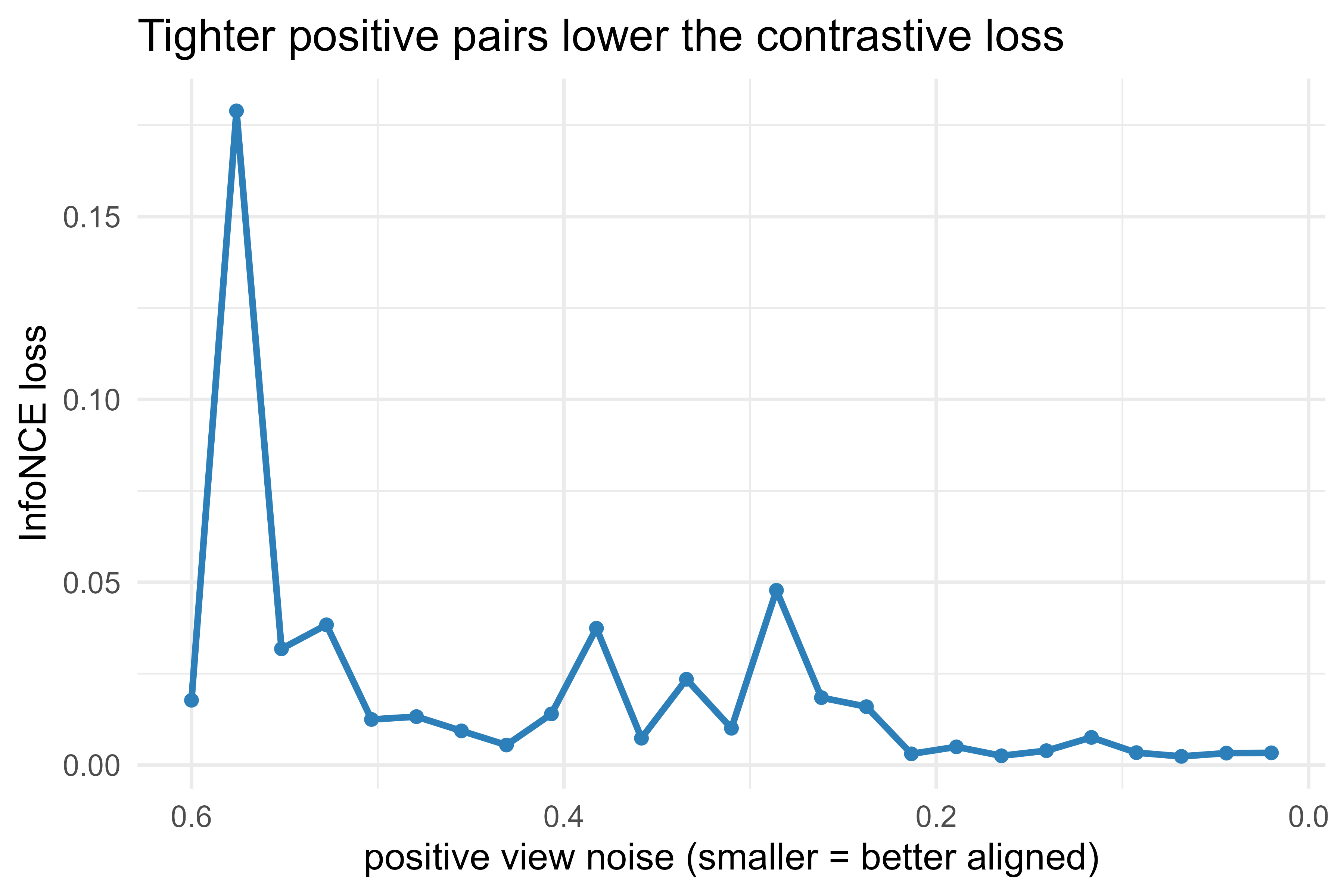
To see the alignment pressure directly, we vary how closely the positive view matches the query (by shrinking the positive’s noise) and plot the resulting loss. As positives align better, the InfoNCE loss falls. Figure 49.1 shows this relationship.
Show code
library(ggplot2)noise_grid<-seq(0.6, 0.02, length.out =25)set.seed(7)loss_curve<-sapply(noise_grid, function(s){Zq<-make_view(items, noise_sd =0.3)Zp<-make_view(items, noise_sd =s)info_nce(Zq, Zp, tau =0.1)})df<-data.frame(positive_noise =noise_grid, loss =loss_curve)ggplot(df, aes(positive_noise, loss))+geom_line(color ="#2c7fb8", linewidth =1)+geom_point(color ="#2c7fb8", size =1.5)+scale_x_reverse()+labs( x ="positive view noise (smaller = better aligned)", y ="InfoNCE loss", title ="Tighter positive pairs lower the contrastive loss")+theme_minimal(base_size =12)
Figure 49.1: InfoNCE loss as positive views become cleaner copies of the item. Lower noise means tighter alignment of positive pairs and a smaller loss.
The curve falls as the positive noise shrinks, which is the alignment term of the loss at work. The negatives, held at random positions, supply the floor: the loss does not go to zero because the query must still beat real competing items.
49.9 A Minimal Gradient Step on the Contrastive Objective
The experiments above poked at a fixed loss. To show that the loss can actually train a representation, we run a few steps of gradient descent on a tiny linear encoder using a numerical gradient.5 The encoder is a matrix \(W\) that maps raw inputs to representations; we minimize InfoNCE over a batch and watch the loss decrease. This uses only base R.
Show code
set.seed(3)n<-8; p<-10; d<-4raw_items<-matrix(rnorm(n*p), nrow =n)# build two raw views by adding noise in input spaceraw_view<-function(items, sd)items+matrix(rnorm(length(items), sd =sd), nrow =nrow(items))X1<-raw_view(raw_items, 0.3)X2<-raw_view(raw_items, 0.3)# encoder is a p x d matrix; representation = X %*% Wloss_W<-function(W, tau=0.1){Z<-X1%*%matrix(W, nrow =p)Zpos<-X2%*%matrix(W, nrow =p)info_nce(Z, Zpos, tau =tau)}W<-rnorm(p*d, sd =0.5)# flattened weightslr<-0.5eps<-1e-4trace<-numeric(40)for(stepinseq_len(40)){base<-loss_W(W)trace[step]<-basegrad<-numeric(length(W))for(jinseq_along(W)){# finite-difference gradientWj<-W; Wj[j]<-Wj[j]+epsgrad[j]<-(loss_W(Wj)-base)/eps}W<-W-lr*grad}c(loss_start =round(trace[1], 4), loss_end =round(loss_W(W), 4))#> loss_start loss_end #> 0.6403 0.0106
The loss drops over the steps, which means the encoder \(W\) has learned a linear map under which the two views of each item land near each other and away from other items. That is a representation trained with no labels, only the positive-and-negative structure built from the data.
49.10 Practical Guidance and Pitfalls
The methods differ in detail, but the failure modes and tuning levers are shared. The guidance below is organized from “should I use this at all” down to the knobs you turn once you have committed.
When self-supervised learning pays off. Reach for it when unlabeled data is abundant and labels are scarce or expensive, when you need one representation to serve several downstream tasks, or when a public pretrained checkpoint already exists for your modality. If you have plenty of labels for a single fixed task, plain supervised learning is usually simpler and at least as good.
Augmentations are the design surface for contrastive methods. The representation keeps what is invariant across views, so the choice of transformations decides what the representation ignores. Augmentations that are too weak make the positive task trivial and the features uninformative. Augmentations that destroy the content (for example, a crop that removes the object) create false positives and corrupt training. Tuning augmentations is often more important than tuning the network.
Watch for collapse. If all representations drift to one point, contrastive loss falls but the features are useless. Symptoms include very low loss with near-zero variance across a batch and a linear probe that performs at chance. Monitor the standard deviation of representations and the rank of their covariance, not just the loss.
Warning
A falling loss is not proof of progress. The cheapest way for any of these methods to lower the loss is to collapse, and a collapsed encoder reports a beautiful loss curve right up until you measure the linear probe and find it at chance. Always track a representation-diversity metric alongside the loss.
Negatives and batch size interact. SimCLR needs large batches for enough negatives; if you cannot afford that memory, use MoCo’s queue or a non-contrastive method like BYOL or SimSiam. Beware of false negatives: two different items that are genuinely similar get pushed apart, which can hurt.
Temperature matters. Small \(\tau\) emphasizes hard negatives and can speed learning but is unstable; large \(\tau\) is gentler but may underfit. Treat \(\tau\) as a first-class hyperparameter and tune it.
Evaluate with a frozen linear probe. The standard, comparable measure of representation quality is the accuracy of a linear model on frozen features. Report it before deciding to fine-tune, because a strong probe means the representation already carries the task signal.
The pretext objective is not the metric you care about. A model can ace masked prediction or contrastive matching and still transfer poorly. Always validate on the actual downstream task.
49.10.1 Computational and Sample Complexity
The methods have different cost profiles that should drive the choice under a fixed budget. For a batch of \(N\) items, \(2N\) views, and projection dimension \(m\):
SimCLR forms the full \((2N)\times(2N)\) similarity matrix, so a training step costs \(O(N^2 m)\) time and \(O(N^2)\) memory on top of the encoder forward and backward passes. Doubling the batch quadruples the contrastive overhead, which is why SimCLR is bandwidth-bound at the batch sizes (4096 and up) where it performs best.
MoCo costs \(O(N K m)\) for the query-to-queue similarities with queue size \(K\), plus \(O(K m)\) memory for the queue. Because \(K\) is decoupled from \(N\), MoCo reaches the same effective negative count at a fraction of the memory, paying instead with the second (momentum) encoder forward pass.
BYOL and SimSiam cost two encoder passes and a predictor pass per step, with no quadratic term, so per-step cost is roughly linear in \(N\). Their expense is wall-clock training length and sensitivity to tuning, not per-step memory.
Masked modeling costs one forward and backward pass over the (possibly shortened) sequence. MAE exploits its high mask ratio by feeding only the visible 25 percent of patches to the encoder, cutting encoder cost by roughly \(4\times\) relative to processing the full image, with a lightweight decoder reconstructing the rest.
On the statistical side, contrastive theory gives a downstream guarantee of the following shape. If the pretrained representation achieves contrastive risk \(\mathcal{L}\) and there are \(C\) latent classes, then a linear classifier on the frozen features has supervised risk bounded (up to constants and a class-collision term that shrinks as classes separate) by a quantity that decreases with \(\mathcal{L}\) and increases with \(\log C\). The practical reading is that more negatives reduce the gap between the contrastive surrogate and the true classification objective only up to the point where false negatives (negatives that share the latent class of the query) begin to dominate the collision term. This is the formal counterpart to the false-negative warning above: beyond a modality-dependent \(K\), adding negatives stops helping because too many of them are secretly positives.
49.10.2 Choosing Hyperparameters
The levers, in rough order of impact:
Augmentation strength: the single most important choice for contrastive methods, as argued above. Calibrate so the positive task is nontrivial but the object survives. Random resized crop plus color jitter is the standard image recipe; the crop scale lower bound is the most sensitive knob.
Temperature \(\tau\): tune on a small grid around \(0.1\) (try \(0.05, 0.1, 0.2\)). Use Equation 49.6 to reason about it: lower \(\tau\) if the model underfits hard cases, raise it if training is unstable.
Batch size or queue size \(K\): set as large as memory allows for SimCLR; for MoCo decouple and set \(K\) in the \(10^3\) to \(10^5\) range, capped before false negatives dominate.
Momentum \(m\) (MoCo, BYOL): keep near \(0.99\) to \(0.999\); it should be large enough that the target moves slower than the queue turnover.
Projection head: a two- or three-layer MLP with the representation taken from before it. Discarding the head at transfer time is consistently better than keeping it, because the head specializes to the contrastive task.
49.11 A Larger Encoder With Keras (Not Run Here)
The base-R demonstration uses a linear encoder and a finite-difference gradient so the idea is transparent. A real contrastive setup uses a deep encoder, a projection head, and automatic differentiation. The code below sketches a SimCLR-style training step in Keras. It is set eval=FALSE because it needs the Python backend, but it is the idiomatic shape of such a model.
Show code
library(keras)library(tensorflow)input_dim<-64Lproj_dim<-32Ltau<-0.1# encoder plus projection headmake_encoder<-function(){keras_model_sequential()|>layer_dense(256, activation ="relu", input_shape =input_dim)|>layer_dense(256, activation ="relu")|>layer_dense(proj_dim)}encoder<-make_encoder()# NT-Xent / InfoNCE loss for a batch of 2N projected, l2-normalized viewsnt_xent<-function(z1, z2, tau){z1<-tf$math$l2_normalize(z1, axis =1L)z2<-tf$math$l2_normalize(z2, axis =1L)z<-tf$concat(list(z1, z2), axis =0L)# shape (2N, proj_dim)sim<-tf$matmul(z, z, transpose_b =TRUE)/tau# (2N, 2N)n2<-tf$shape(z)[1]# mask out self-similarity on the diagonalmask<-tf$eye(n2)*-1e9sim<-sim+maskN<-tf$shape(z1)[1]# positive of row i is its partner viewtargets<-tf$concat(list(tf$range(N)+N, tf$range(N)), axis =0L)loss<-tf$nn$sparse_softmax_cross_entropy_with_logits(labels =targets, logits =sim)tf$reduce_mean(loss)}optimizer<-optimizer_adam(learning_rate =1e-3)train_step<-function(view1, view2){with(tf$GradientTape()%as%tape, {z1<-encoder(view1)z2<-encoder(view2)loss<-nt_xent(z1, z2, tau)})grads<-tape$gradient(loss, encoder$trainable_variables)optimizer$apply_gradients(purrr::transpose(list(grads, encoder$trainable_variables)))loss}# for (batch in dataset) train_step(batch$view1, batch$view2)
49.12 Summary
The thread tying this chapter together is that a learning signal can come from the structure of the data instead of from labels. Pretext tasks invent a puzzle and hope useful features fall out. Contrastive methods make that hope precise: pull views of the same item together, push different items apart, and (through the InfoNCE bound) keep the information shared across views. SimCLR and MoCo are two ways to supply the negatives that prevent collapse, BYOL and SimSiam show negatives are not strictly required if a predictor and stop-gradient break the symmetry, and masked modeling sidesteps the whole question by reconstructing hidden parts of the input. Across all of them the workflow is the same: pretrain once, then probe or fine-tune with the few labels you have. When you apply these methods, judge the representation by a frozen linear probe on the real task, not by the pretext loss, and keep an eye out for collapse the entire way.
49.13 Further Reading
Oord, Li, and Vinyals (2018), “Representation Learning with Contrastive Predictive Coding,” introduce the InfoNCE objective and the mutual-information lower bound.
Chen, Kornblith, Norouzi, and Hinton (2020), “A Simple Framework for Contrastive Learning of Visual Representations” (SimCLR), study augmentations, the projection head, temperature, and batch size.
He, Fan, Wu, Xie, and Girshick (2020), “Momentum Contrast for Unsupervised Visual Representation Learning” (MoCo), introduce the queue of negatives and the momentum encoder.
Grill and colleagues (2020), “Bootstrap Your Own Latent” (BYOL), show that strong representations can be learned without negative pairs.
Chen and He (2021), “Exploring Simple Siamese Representation Learning” (SimSiam), isolate the stop-gradient and predictor as the ingredients that prevent collapse.
Devlin, Chang, Lee, and Toutanova (2019), “BERT: Pre-training of Deep Bidirectional Transformers for Language Understanding,” establish masked language modeling for text.
He, Chen, Xie, Li, Dollar, and Girshick (2022), “Masked Autoencoders Are Scalable Vision Learners” (MAE), show high-ratio masked reconstruction for images.
Wang and Isola (2020), “Understanding Contrastive Representation Learning through Alignment and Uniformity on the Hypersphere,” give the alignment-and-uniformity decomposition of the contrastive loss.
A shortcut is a low-level cue that solves the pretext task without requiring the semantic understanding you were hoping to induce. Chromatic aberration at image edges, for instance, can reveal a patch’s original position and let a jigsaw solver cheat.↩︎
The projection head is a small network applied only during pretraining; the representation used downstream is taken from before it. Normalizing to the unit sphere means the dot product equals the cosine of the angle between two vectors, so similarity ranges from \(-1\) to \(1\) and does not depend on vector length.↩︎
Mutual information \(I(z; z^{+})\) measures how much knowing one view tells you about the other, in bits or nats. The inequality is a lower bound: minimizing the loss cannot prove the information is high, but it does rule out it being low.↩︎
Stop-gradient means we treat the target’s output as a fixed constant during backpropagation: gradients flow through the online branch only. The target’s weights then change slowly through the moving average, not through the loss.↩︎
We use a finite-difference gradient: nudge each weight by a tiny \(\varepsilon\) and measure how the loss changes. Real systems use automatic differentiation, which is exact and far faster, but the finite-difference version keeps the code short and free of extra packages.↩︎
Source Code
# Self-Supervised and Contrastive Learning {#sec-self-supervised-learning}```{r}#| include: falsesource("_common.R")```Self-supervised learning trains a model to predict some part of its input from another part, using the structure of unlabeled data as the supervision signal. There are no human labels. The labels are constructed automatically from the data itself, which is why the approach scales to the large unlabeled corpora that data teams already hold. The output of self-supervised training is not a classifier or a regressor. It is a learned representation: a function that maps raw inputs to vectors that make downstream tasks easier. Once a good representation exists, a small labeled dataset and a simple model (often a linear layer) are enough to solve the task you actually care about.This chapter covers the main families of self-supervised methods used in practice: pretext tasks, contrastive learning with the InfoNCE objective, the SimCLR and MoCo training recipes, the non-contrastive BYOL approach, and masked modeling as used by BERT and masked autoencoders. The recurring question is why a representation learned without labels transfers to tasks that have labels. We work through the InfoNCE loss in detail and give a runnable base-R demonstration that shows exactly how positive and negative pairs move the loss.::: {.callout-important title="Key idea"}Self-supervised learning does not solve your task directly. It learns a *representation*, a reusable map from raw input to a vector, and a small labeled step turns that representation into the model you need. Keep the two stages separate in your mind: learning the map, then using the map.:::::: {.callout-note}"Self-supervised" and "unsupervised" are often used loosely, but they are not the same. Unsupervised learning (clustering, covered in @sec-cluster, and density estimation, covered in @sec-density-estimation) has no target at all. Self-supervised learning invents a target from the input, so the machinery of supervised training (a loss, gradients, a prediction) still applies; only the labels are free.:::## Where This Fits in a Modern WorkflowMost teams sit on far more unlabeled data than labeled data. Logs, images, documents, sensor traces, and user events accumulate continuously, while labeling is slow and expensive. Self-supervised learning turns the cheap, abundant resource into a pretrained representation, and reserves the scarce labels for a short fine-tuning step.A typical pipeline has three stages.1. Pretrain. Train an encoder $f_\theta$ on unlabeled data with a self-supervised objective. This is the expensive step and it is done once, often by a separate team or downloaded as a public checkpoint.2. Transfer. Freeze or lightly fine-tune $f_\theta$ and attach a small task head. With frozen features this is called *linear probing*: fit a linear model on top of $f_\theta(x)$. The quality of the representation is often reported as the accuracy of this linear probe.3. Fine-tune. If labels are plentiful enough, unfreeze the encoder and train the whole stack at a low learning rate so the representation adapts to the task.::: {.callout-tip}Most practitioners never run stage 1. The expensive pretraining is done once by a well-resourced lab and released as a public checkpoint, so your day-to-day work is stages 2 and 3 on top of someone else's encoder. Knowing how the encoder was trained still matters, because it tells you what the representation is invariant to and therefore what it will quietly ignore.:::This is the same shape as the transfer-learning workflow (@sec-transfer-multitask-learning) behind BERT (@sec-bert) for text and pretrained vision backbones for images. The difference from supervised pretraining is only the source of the training signal: the structure of the data instead of external labels.## Pretext TasksThe earliest self-supervised methods invent a *pretext task*: a supervised problem whose labels are free because they come from the data. Solving the pretext task well is not the goal. The goal is that the features the model builds while solving it are useful for real tasks.Examples that shaped the field:- Context prediction. Given two image patches, predict their relative spatial arrangement. To answer, the model must recognize object parts and their layout.- Rotation prediction. Rotate an image by $0, 90, 180,$ or $270$ degrees and predict the angle. Getting this right requires knowing the canonical orientation of objects.- Colorization. Remove color and predict it back. The model has to associate textures and shapes with plausible colors.- Jigsaw puzzles. Shuffle image tiles and predict the permutation.The weakness of hand-designed pretext tasks is that the model can exploit shortcuts.^[A *shortcut* is a low-level cue that solves the pretext task without requiring the semantic understanding you were hoping to induce. Chromatic aberration at image edges, for instance, can reveal a patch's original position and let a jigsaw solver cheat.] A rotation predictor might key on watermarks or sky-at-top cues rather than object structure. Contrastive and masked methods, covered next, are more robust because the supervision is harder to game.::: {.callout-tip title="Intuition"}A pretext task is a teacher who sets a puzzle hoping the student learns something general while solving it. The risk is the same as in a classroom: the student may find a trick that aces the puzzle and teaches nothing. The methods that follow design puzzles where the only winning strategy is to actually understand the content.:::## Contrastive Learning and the InfoNCE ObjectiveContrastive learning replaces a single hand-built pretext task with a general principle: representations of two views of the same item should be close, and representations of different items should be far apart. "Close" and "far" are measured by a similarity in the representation space.### Views and the SimilarityStart with an input $x$ and apply two random transformations to get two *views*, $\tilde x$ and $\tilde x^{+}$. For images the transformations are crops, color shifts, and blurs. For text they can be token masking or dropout. The pair $(\tilde x, \tilde x^{+})$ is a *positive pair*: two views of the same underlying item. Views of other items in the batch are *negatives*.An encoder $f_\theta$ maps a view to a vector, usually followed by a small projection head and an $\ell_2$ normalization so that every representation lies on the unit sphere.^[The *projection head* is a small network applied only during pretraining; the representation used downstream is taken from before it. Normalizing to the unit sphere means the dot product equals the cosine of the angle between two vectors, so similarity ranges from $-1$ to $1$ and does not depend on vector length.] Write the normalized representations as $z = f_\theta(\tilde x)$ and $z^{+} = f_\theta(\tilde x^{+})$ with $\lVert z \rVert = 1$. Similarity is the dot product (cosine similarity on the unit sphere),$$\operatorname{sim}(u, v) = u^\top v .$$### The LossConsider a query $z$ with one positive $z^{+}$ and a set of negatives $\{z^{-}_1, \dots, z^{-}_K\}$. The InfoNCE loss, also called the normalized temperature-scaled cross-entropy loss, is$$\ell(z) = -\log \frac{\exp(z^\top z^{+} / \tau)}{\exp(z^\top z^{+} / \tau) + \sum_{k=1}^{K} \exp(z^\top z^{-}_k / \tau)} .$$The temperature $\tau > 0$ scales the similarities before the softmax. Read the fraction as a classification problem: among the $K+1$ candidates (one positive and $K$ negatives), which one is the true match for $z$? The loss is the cross-entropy of a softmax classifier that has to pick the positive. Minimizing it pushes $z^\top z^{+}$ up and pushes each $z^\top z^{-}_k$ down.::: {.callout-tip title="Intuition"}Picture a lineup. The query $z$ is shown a row of candidates, exactly one of which is its partner view. InfoNCE rewards the encoder for confidently fingering the right partner. To win this game across many lineups, the encoder has no choice but to place each item's two views near each other and away from everyone else.:::The temperature controls how sharply the loss focuses on the hardest negatives. Small $\tau$ makes the softmax sharp, so negatives with high similarity to the query dominate the gradient. Large $\tau$ flattens the distribution and treats all negatives more equally. In practice $\tau$ is a sensitive hyperparameter, often near $0.1$.### Why It Learns a Useful RepresentationInfoNCE has an information-theoretic reading. Let $z$ and $z^{+}$ be representations of two views that share the same latent content. Minimizing the expected InfoNCE loss with $K$ negatives maximizes a lower bound on the mutual information between the two views,$$I(z; z^{+}) \; \ge \; \log(K+1) - \mathcal{L}_{\text{InfoNCE}} .$$The bound says the loss is a budget: pushing $\mathcal{L}_{\text{InfoNCE}}$ down raises the guaranteed floor on the shared information $I(z; z^{+})$, and more negatives ($K$ large) raise the ceiling $\log(K+1)$ that the floor can reach.^[Mutual information $I(z; z^{+})$ measures how much knowing one view tells you about the other, in bits or nats. The inequality is a *lower bound*: minimizing the loss cannot prove the information is high, but it does rule out it being low.] So driving the loss down forces the representation to keep whatever information is shared across views and discard what is not. The transformations are chosen so that the shared content is the semantic identity of the item (the object in an image, the meaning of a sentence) and the discarded part is nuisance variation (crop position, color jitter, exact wording). That is the mechanism behind transfer: the representation retains task-relevant structure because that structure is what survives across views, and it drops the nuisance factors that a downstream task would also want to ignore.A second, more geometric view comes from decomposing the loss. Writing it out, InfoNCE pushes for *alignment* (positives close) and *uniformity* (representations spread over the sphere so they stay distinguishable). The negatives supply the uniformity pressure. Without them, the encoder could map every input to the same point, drive all positive similarities to one, and make the loss small while learning nothing. This failure is called *representation collapse*, and avoiding it is the central design problem for the methods below.### Formal Setup and the Loss as a Conditional LikelihoodTo make the objective precise, fix the data-generating process. Let $x$ be drawn from the data distribution $p(x)$, and let a stochastic augmentation $t \sim \mathcal{T}$ produce a view $\tilde x = t(x)$. Two independent draws $t, t' \sim \mathcal{T}$ give the positive pair $(\tilde x, \tilde x^{+})$. The encoder $g_\theta$ (encoder plus projection head) maps a view to $\mathbb{R}^m$, and we normalize $z = g_\theta(\tilde x)/\lVert g_\theta(\tilde x)\rVert$ so that $z \in \mathcal{S}^{m-1}$, the unit sphere. The temperature $\tau>0$ is fixed.InfoNCE is exactly the negative log-likelihood of a softmax classifier whose job is to pick the positive out of a candidate set of size $K+1$. Index the candidates $0,1,\dots,K$ with candidate $0$ the positive. Define the categorical model$$p_\theta(\,\text{match}=0 \mid z, \{z_j\}_{j=0}^{K}) = \frac{\exp(z^\top z_0/\tau)}{\sum_{j=0}^{K}\exp(z^\top z_j/\tau)} .$$ {#eq-self-supervised-learning-softmax}The loss $\ell(z) = -\log p_\theta(\text{match}=0\mid \cdot)$ in @eq-self-supervised-learning-softmax reproduces the InfoNCE loss above. Reading it as a $(K+1)$-way classification makes the connection to cross-entropy literal: the network outputs logits $z^\top z_j/\tau$ and the free label is "the positive sits in slot $0$."### Derivation: InfoNCE as a Mutual-Information Lower BoundWe now derive the bound $I(z;z^{+}) \ge \log(K+1) - \mathcal{L}_{\text{InfoNCE}}$ stated above, following the contrastive predictive coding argument. The key is that the optimal critic recovers a density ratio.Consider one positive sample drawn from the joint $p(z, z^{+})$ and $K$ negatives drawn independently from the marginal $p(z^{+})$. Collect the $K+1$ candidates in $Z=\{z_0,\dots,z_K\}$, with the positive placed uniformly at a random slot. The posterior probability that slot $i$ holds the positive, given $z$ and $Z$, is by Bayes' rule$$p(\text{pos}=i \mid z, Z) = \frac{p(z_i \mid z)\prod_{j\ne i} p(z_j)}{\sum_{k=0}^{K} p(z_k\mid z)\prod_{j\ne k}p(z_j)} = \frac{\dfrac{p(z_i\mid z)}{p(z_i)}}{\sum_{k=0}^{K}\dfrac{p(z_k\mid z)}{p(z_k)}} ,$$ {#eq-self-supervised-learning-bayes}where the second equality divides numerator and denominator by $\prod_{j} p(z_j)$. The Bayes-optimal classifier therefore scores each candidate by the density ratio $r(z_i, z) = p(z_i\mid z)/p(z_i) = p(z, z_i)/(p(z)p(z_i))$. Comparing with @eq-self-supervised-learning-softmax, the softmax classifier is Bayes-optimal exactly when the learned similarity matches the log density ratio up to a $z$-dependent constant,$$\exp(z^\top z_i/\tau) \;\propto\; \frac{p(z, z_i)}{p(z)\,p(z_i)} .$$ {#eq-self-supervised-learning-ratio}Now substitute the optimal critic into the expected loss. With the positive at slot $0$,$$\mathcal{L}_{\text{InfoNCE}} = -\,\mathbb{E}\!\left[\log \frac{r(z_0,z)}{\sum_{k=0}^{K} r(z_k, z)}\right]= \mathbb{E}\!\left[\log\left(1 + \frac{p(z_0)}{p(z_0\mid z)}\sum_{k=1}^{K} \frac{p(z_k\mid z)}{p(z_k)}\right)\right].$$The $K$ negative terms are i.i.d. draws from the marginal, so $\mathbb{E}_{z_k}\big[p(z_k\mid z)/p(z_k)\big]=\int p(z_k\mid z)\,dz_k = 1$. By the law of large numbers the inner sum concentrates on its mean, $\sum_{k=1}^{K} p(z_k\mid z)/p(z_k) \approx K\,\mathbb{E}_{z_k}\big[p(z_k\mid z)/p(z_k)\big] = K$ (this concentration approximation, not Jensen, is the step that makes the argument non-rigorous), which yields$$\mathcal{L}_{\text{InfoNCE}} \;\approx\; \mathbb{E}\!\left[\log\left(1 + \frac{p(z_0)}{p(z_0\mid z)}\,K\right)\right] \;\ge\; \mathbb{E}\!\left[\log \frac{p(z_0)}{p(z_0\mid z)} K\right] = \log K - I(z; z^{+}).$$Rearranging gives the advertised bound, with $\log(K+1)$ in place of $\log K$ when the positive slot is counted among the $K+1$ candidates,$$I(z; z^{+}) \;\ge\; \log(K+1) - \mathcal{L}_{\text{InfoNCE}} .$$ {#eq-self-supervised-learning-mi-bound}Two consequences follow immediately from @eq-self-supervised-learning-mi-bound. First, the bound is loose by at most $\log(K+1)$, so it can certify at most $\log(K+1)$ nats of mutual information; this is the precise sense in which more negatives raise the ceiling. Second, if the true $I(z;z^{+})$ exceeds $\log(K+1)$, the loss cannot be driven to zero no matter how good the encoder, which is why InfoNCE saturates and why large $K$ matters for high-information modalities.::: {.callout-warning title="The bias of the bound"}@eq-self-supervised-learning-mi-bound is a *lower* bound on $I(z;z^{+})$, so minimizing the loss is a surrogate, not a direct maximization of mutual information. The slack $\log(K+1)-\mathcal{L}$ is what you actually control. Estimators of mutual information based on this bound are known to have variance and bias that grow with the true information, so InfoNCE is best read as a representation objective whose MI interpretation is a guide, not a guarantee.:::### Derivation: The Alignment and Uniformity DecompositionThe geometric picture can be made exact in the limit of infinitely many negatives. Write the per-sample loss with negatives drawn from the marginal $p_z$ over the sphere,$$\ell(z) = -\frac{z^\top z^{+}}{\tau} + \log\!\left(\exp(z^\top z^{+}/\tau) + \sum_{k=1}^{K}\exp(z^\top z^{-}_k/\tau)\right).$$Take expectations and let $K\to\infty$. The first term becomes the negative expected positive similarity, and by the law of large numbers the sum inside the log concentrates on $K\,\mathbb{E}_{z^-}\exp(z^\top z^-/\tau)$. Dropping the additive $\log K$ constant, the asymptotic objective splits into two pieces,$$\mathcal{L}_\infty(\theta) = \underbrace{-\frac{1}{\tau}\,\mathbb{E}_{(z,z^{+})}\,z^\top z^{+}}_{\text{alignment}} \;+\; \underbrace{\mathbb{E}_{z}\,\log \mathbb{E}_{z^{-}}\exp(z^\top z^{-}/\tau)}_{\text{uniformity}} .$$ {#eq-self-supervised-learning-align-unif}The alignment term is minimized when positive pairs are identical on the sphere. The uniformity term in @eq-self-supervised-learning-align-unif is, up to constants, the logarithm of the Gaussian-kernel potential $\mathbb{E}\,e^{-\lVert z - z^{-}\rVert^2/(2\tau)\cdot c}$ (using $\lVert z-z^-\rVert^2 = 2-2z^\top z^-$ on the unit sphere). Minimizing it spreads the representations as uniformly as possible over $\mathcal{S}^{m-1}$; its global minimizer is the uniform distribution on the sphere. This is the formal statement that negatives supply *uniformity* pressure and positives supply *alignment* pressure, and it explains collapse directly: with no negatives the uniformity term vanishes and the alignment term alone is minimized by the constant map.### Derivation: The InfoNCE Gradient and Hard-Negative WeightingTo see *why* small temperature emphasizes hard negatives, differentiate. With $s_j = z^\top z_j/\tau$ and softmax weights $p_j = e^{s_j}/\sum_k e^{s_k}$ over the candidates (positive at slot $0$), the loss is $\ell = -s_0 + \log\sum_j e^{s_j}$, so$$\frac{\partial \ell}{\partial z} = -\frac{z_0}{\tau} + \sum_{j} p_j\,\frac{z_j}{\tau} = \frac{1}{\tau}\Big[(p_0-1)\,z_0 + \sum_{k\ge 1} p_k\, z_k\Big].$$ {#eq-self-supervised-learning-grad}The gradient pulls $z$ toward the positive (the $(p_0-1)z_0$ term, since $p_0-1<0$) and pushes it away from each negative with weight $p_k$. Because $p_k \propto e^{z^\top z_k/\tau}$, a hard negative (large $z^\top z_k$) receives an exponentially larger repulsion weight as $\tau\to 0$. Thus small $\tau$ concentrates the gradient on the few hardest negatives, sharpening the decision boundary but increasing variance; large $\tau$ averages over all negatives, which is gentler but blurs the contrast. This is the analytic content behind the earlier remark that $\tau$ trades hard-negative focus against stability.::: {.callout-warning}Collapse is the recurring villain of self-supervised learning. Watch for it whenever a method has alignment pressure but weak or no uniformity pressure. The two terms are in tension: alignment alone wants to crush everything together, uniformity alone wants to scatter it, and a good representation is the balance between them.:::## SimCLR and MoCo: Two Ways to Get NegativesInfoNCE needs many negatives to give a strong uniformity signal and a tight mutual-information bound. The two influential recipes differ mainly in where the negatives come from.SimCLR uses the other items in the current minibatch as negatives. For a batch of $N$ items it makes two views of each, giving $2N$ views; for any view its positive is the other view of the same item and the remaining $2N-2$ views are negatives. This is simple and has no extra moving parts, but it needs large batches (thousands) to have enough negatives, which costs memory.MoCo (Momentum Contrast) decouples the number of negatives from the batch size. It keeps a queue of representations from recent batches to act as negatives, so the effective negative set is large even with a modest batch. The negatives are encoded by a second *momentum encoder* whose weights are an exponential moving average of the main encoder,$$\theta_{\text{key}} \leftarrow m \, \theta_{\text{key}} + (1 - m)\, \theta_{\text{query}}, \qquad m \in [0, 1) \text{ close to } 1 .$$The slow-moving key encoder keeps the queued representations consistent over time, which matters because they were computed by slightly older weights.### SimCLR: the NT-Xent Loss Made PreciseIn a SimCLR batch of $N$ items, augmentation produces $2N$ views indexed $i=1,\dots,2N$, where view $i$ and its partner $j(i)$ are the two views of the same item. With normalized projections $z_i$ and similarity $s_{ik}=z_i^\top z_k/\tau$, the per-view NT-Xent loss excludes self-comparison,$$\ell_i = -\log \frac{\exp(s_{i,j(i)})}{\sum_{k=1}^{2N}\mathbb{1}[k\ne i]\,\exp(s_{ik})},\qquad\mathcal{L}_{\text{SimCLR}} = \frac{1}{2N}\sum_{i=1}^{2N}\ell_i .$$ {#eq-self-supervised-learning-ntxent}Each view in @eq-self-supervised-learning-ntxent sees $K = 2N-2$ negatives, so the effective negative count is tied directly to batch size; this is why SimCLR needs batches in the thousands to make the $\log(K+1)$ ceiling in @eq-self-supervised-learning-mi-bound useful. The cost is the $(2N)\times(2N)$ similarity matrix, which is $O(N^2 m)$ to form and $O(N^2)$ memory, dominating large-batch training. The loss is symmetric in the two views because every view serves as a query.### MoCo as a Dictionary Lookup and the Role of MomentumMoCo reframes contrastive learning as lookup against a dictionary. The query $q=g_{\theta_q}(\tilde x)$ is matched against keys $\{k_0,k_1,\dots\}$, where $k_0$ is the positive key and the rest come from a FIFO queue of size $K$ encoded by the momentum encoder. The loss is the single-query InfoNCE,$$\ell_{\text{MoCo}} = -\log \frac{\exp(q^\top k_0/\tau)}{\sum_{i=0}^{K}\exp(q^\top k_i/\tau)} .$$Decoupling $K$ from batch size is the central trick: the queue accumulates negatives across many past steps, so $K$ can be tens of thousands with a batch of a few hundred. The momentum update $\theta_{\text{key}} \leftarrow m\,\theta_{\text{key}} + (1-m)\,\theta_{\text{query}}$ is what makes this safe. If the key encoder were updated by gradient like the query encoder, the queued keys would be stale: representations computed several hundred steps ago by rapidly changing weights would no longer be comparable to current queries, and training would diverge. The slow update keeps the key encoder approximately constant over the lifetime of the queue. Concretely, a key enters the queue and is evicted after $K/\,(\text{batch size})$ steps; over that span $\theta_{\text{key}}$ moves by roughly a factor $1-m^{K/\text{batch}}$, so $m$ near $0.999$ keeps the dictionary consistent. Empirically large $m$ (0.99 to 0.999) is essential; $m=0$ (no momentum, key encoder equals query encoder) collapses performance.::: {.callout-tip title="When to use this"}Choose SimCLR when you can afford large batches and want the simplest pipeline. Choose MoCo when GPU memory caps your batch size but you still want many negatives; its queue lets a small batch see thousands of negatives accumulated over recent steps.:::## BYOL: Contrastive Without NegativesBYOL (Bootstrap Your Own Latent) removes negatives entirely and still avoids collapse. At first glance this should be impossible: with no negatives, what stops the encoder from mapping everything to one point? That puzzle is exactly what makes BYOL interesting. It uses two networks: an *online* network and a *target* network. The online network sees one view and is asked to predict the target network's representation of the other view. The target network is again an exponential moving average of the online network and is not trained by gradients.^[*Stop-gradient* means we treat the target's output as a fixed constant during backpropagation: gradients flow through the online branch only. The target's weights then change slowly through the moving average, not through the loss.]The objective is a regression toward the target representation, typically the squared error between $\ell_2$-normalized vectors,$$\mathcal{L}_{\text{BYOL}} = \big\lVert \, \overline{q(z)} - \overline{z^{+}_{\text{target}}} \, \big\rVert^2 ,$$where $q$ is a predictor on the online side and the bar denotes normalization. Two ingredients keep the trivial constant solution away: the extra predictor $q$ on only the online side breaks the symmetry between the two branches, and the stop-gradient on the target branch means the target does not chase the online network. The result is competitive with contrastive methods without ever forming a negative pair, which removes the large-batch and queue machinery. A related method, SimSiam, shows that even the moving-average target can be dropped if the stop-gradient and predictor are kept.### Why BYOL Does Not Collapse: the Stop-Gradient ArgumentIt is worth being precise about the puzzle, because the resolution is subtle and the naive analysis predicts collapse. Expand the BYOL objective with online encoder $f_\theta$, predictor $q_\theta$, target encoder $f_\xi$, and stop-gradient $\operatorname{sg}$,$$\mathcal{L}_{\text{BYOL}}(\theta) = \mathbb{E}\,\big\lVert \overline{q_\theta(f_\theta(\tilde x))} - \operatorname{sg}\big(\overline{f_\xi(\tilde x^{+})}\big)\big\rVert^2 .$$The constant map ($f$ outputs a fixed vector) is a global minimizer with loss zero, so nothing in the objective forbids collapse. SimSiam analyzes why gradient descent nonetheless avoids it by reading the procedure as alternating optimization of an auxiliary problem. Introduce a per-image latent target $\eta_x$ and the surrogate$$\mathcal{L}(\theta, \eta) = \mathbb{E}_x\big\lVert q_\theta(f_\theta(\tilde x)) - \eta_x \big\rVert^2 .$$Holding $\theta$ fixed, the optimal $\eta_x$ is the expectation $\mathbb{E}_{t}\,f_\theta(t(x))$, which is what the stop-gradient branch (with its slow target) approximates. Holding $\eta$ fixed, a gradient step updates $\theta$. The stop-gradient is exactly what makes this an alternating two-variable minimization rather than a single joint descent that would collapse. The predictor $q_\theta$ is the second guard: because the optimal predictor outputs the conditional mean $q^\star(f_\theta(\tilde x)) = \mathbb{E}_{\tilde x^{+}}[\,\overline{f_\xi(\tilde x^{+})}\mid f_\theta(\tilde x)\,]$, it absorbs the augmentation-induced variance and removes the gradient pressure that would otherwise shrink all representations to a point. Remove either ingredient and BYOL collapses, which the SimSiam ablations confirm. The exponential-moving-average target adds stability but is not strictly necessary once stop-gradient and predictor are present.::: {.callout-note title="Connection to contrastive methods"}BYOL has no explicit uniformity term, so it cannot be analyzed through @eq-self-supervised-learning-align-unif. Its anti-collapse mechanism is dynamical (a property of the optimization path) rather than a property of the loss landscape. This is why BYOL is more sensitive to architectural details such as batch-norm in the predictor and projector: those layers inject the implicit between-sample interaction that negatives supply explicitly in SimCLR and MoCo.:::## Masked ModelingMasked modeling is the dominant self-supervised approach for text and a strong one for images. The pretext task is to hide part of the input and reconstruct it from the rest.- Masked language modeling, used by BERT (@sec-bert), replaces a fraction of tokens with a `[MASK]` symbol and trains the model to predict the originals from the surrounding context. Because the model sees both left and right context, it learns bidirectional representations of meaning.- Masked image modeling, used by the masked autoencoder (MAE), splits an image into patches, hides a large fraction (often 75 percent), and reconstructs the missing pixels from the visible patches. The high mask ratio forces the model to learn global structure rather than copy nearby pixels.::: {.callout-tip title="Intuition"}Masked modeling is fill-in-the-blank. To guess the word hidden in "the cat sat on the ___," you need to understand the sentence, not just memorize letter frequencies. The reconstruction target is the original input itself, so there is nothing to collapse onto and no negatives to mine; the difficulty of the blanks does all the work.:::### Masked Modeling as Conditional LikelihoodMasked modeling has a clean likelihood formulation. Let $x = (x_1,\dots,x_L)$ be a sequence (tokens or patches) and let $M\subset\{1,\dots,L\}$ be a random mask with each position included independently with probability $\rho$ (the *mask ratio*). Write $x_M$ for the masked entries and $x_{\setminus M}$ for the visible ones. Masked language modeling maximizes the expected conditional log-likelihood of the masked entries given the visible context,$$\mathcal{L}_{\text{MLM}}(\theta) = -\,\mathbb{E}_{x}\,\mathbb{E}_{M}\,\frac{1}{|M|}\sum_{i\in M} \log p_\theta(x_i \mid x_{\setminus M}) .$$ {#eq-self-supervised-learning-mlm}This is a *pseudo-likelihood* objective: rather than modeling the full joint $p(x)$, which would require an intractable normalizer over all sequences, @eq-self-supervised-learning-mlm models a collection of conditionals $p_\theta(x_i\mid x_{\setminus M})$, each a tractable softmax over the vocabulary. The connection is exact in the small-mask limit: when $|M|=1$, MLM is precisely the pseudo-likelihood of Besag, whose maximizer is consistent for the joint under mild conditions even though no single conditional determines the joint on its own. Larger mask ratios trade this statistical grounding for a harder, more informative prediction problem; BERT uses $\rho\approx 0.15$ for text, while MAE uses $\rho\approx 0.75$ for images because pixels are far more locally redundant than tokens and a low ratio would let the decoder copy neighbors. There is no collapse failure mode here: the target is the observed input itself, so the objective is bounded below by the data entropy and a constant predictor is heavily penalized.::: {.callout-note title="Why bidirectional context matters"}The conditioning set $x_{\setminus M}$ in @eq-self-supervised-learning-mlm includes positions on both sides of each masked entry, which is what gives BERT its bidirectional representations. This is the structural difference from an autoregressive language model, which factorizes $p(x)=\prod_i p(x_i\mid x_{<i})$ and conditions only on the left. The masked objective sacrifices the ability to generate by ancestral sampling in exchange for representations that see full context, a trade that favors discriminative transfer over generation.:::Masked modeling and contrastive learning sit at two ends of a spectrum. Contrastive methods compare whole-item representations and need carefully designed views and negatives. Masked methods predict missing parts and need a good masking scheme but no negatives and no paired augmentations. Both produce representations that transfer; which works better depends on the modality and the downstream task.## A Comparison of the Methods@tbl-self-supervised-learning-method-comparison summarizes how the families differ on the points that matter when you choose one.| Method | Pretext signal | Needs negatives | Collapse prevention | Main cost driver | Typical modality ||----|----|----|----|----|----|| Pretext task (rotation, jigsaw) | Predict a constructed label | No | Task is supervised | Shortcut features | Images || SimCLR | InfoNCE on two views | Yes (in-batch) | Negatives give uniformity | Large batch size | Images || MoCo | InfoNCE on two views | Yes (queue) | Negatives give uniformity | Queue and momentum encoder | Images || BYOL / SimSiam | Predict target's view | No | Predictor plus stop-gradient | Tuning stability | Images || BERT (masked LM) | Reconstruct masked tokens | No | Reconstruction target | Sequence length | Text || MAE (masked image) | Reconstruct masked pixels | No | Reconstruction target | High mask ratio decode | Images |: Comparison of self-supervised learning families across pretext signal, reliance on negatives, collapse prevention, main cost driver, and typical modality. {#tbl-self-supervised-learning-method-comparison}## Demonstration: InfoNCE on Toy Vectors in Base RThe demonstration builds the InfoNCE loss from scratch on small vectors so the mechanics are visible. We create a few items, make two noisy views of each, normalize, and compute the loss. We then show how the loss responds when the positive is made more similar and when a hard negative is introduced. Everything runs in base R.::: {.callout-note}The point here is not to train a useful model on toy data; it is to watch the loss react to changes you control, so the abstract claims above become concrete numbers. Treat each chunk as a small experiment with a prediction attached.:::```{r infonce-setup}set.seed(1)# l2-normalize the rows of a matrix so each representation lies on the unit spherel2_normalize <-function(M) { norms <-sqrt(rowSums(M^2)) M / norms}# InfoNCE loss for a batch where row i of Z and row i of Zpos form a positive pair.# All other rows of Zpos act as negatives for query i (in-batch negatives, SimCLR style).info_nce <-function(Z, Zpos, tau =0.1) { Z <-l2_normalize(Z) Zpos <-l2_normalize(Zpos)# similarity matrix: S[i, j] = sim(query i, candidate j) S <- (Z %*%t(Zpos)) / tau n <-nrow(Z) losses <-numeric(n)for (i inseq_len(n)) { logits <- S[i, ] # candidate i is the positive for query i m <-max(logits) # log-sum-exp for numerical stability log_denom <- m +log(sum(exp(logits - m))) losses[i] <--(logits[i] - log_denom) }mean(losses)}``````{r infonce-batch}# d-dimensional latent identity for each of n itemsn <-6d <-8items <-matrix(rnorm(n * d), nrow = n)# two views = item identity plus independent noisemake_view <-function(items, noise_sd) { items +matrix(rnorm(length(items), sd = noise_sd), nrow =nrow(items))}Z <-make_view(items, noise_sd =0.3)Zpos <-make_view(items, noise_sd =0.3)loss_baseline <-info_nce(Z, Zpos, tau =0.1)loss_baseline```The baseline loss is well above zero because the views are noisy and the negatives are other random items. Now hold the negatives fixed but make the positive view a cleaner copy of the item. The loss should drop, since the positive becomes easier to identify.```{r infonce-cleaner-positive}Zpos_clean <-make_view(items, noise_sd =0.05) # tighter positiveloss_clean_pos <-info_nce(Z, Zpos_clean, tau =0.1)c(noisy_positive = loss_baseline, clean_positive = loss_clean_pos)```Next, inject a *hard negative*: an item whose view is deliberately placed near query 1's representation. A hard negative competes with the true positive in the denominator and pushes the loss up.```{r infonce-hard-negative}Z2 <- ZZpos2 <- Zpos# overwrite item 2's positive view to sit close to item 1's queryZpos2[2, ] <- Z[1, ] +rnorm(d, sd =0.02)loss_hard_neg <-info_nce(Z2, Zpos2, tau =0.1)c(baseline = loss_baseline, with_hard_negative = loss_hard_neg)```Finally, sweep the temperature to see its effect with the hard negative present. Small $\tau$ sharpens the softmax and lets the hard negative dominate, raising the loss; larger $\tau$ smooths it out.```{r infonce-temperature}taus <-c(0.05, 0.1, 0.2, 0.5, 1.0)loss_by_tau <-sapply(taus, function(t) info_nce(Z2, Zpos2, tau = t))data.frame(tau = taus, loss =round(loss_by_tau, 4))```### Verifying the Mutual-Information Bound NumericallyThe bound @eq-self-supervised-learning-mi-bound says $I(z;z^{+}) \ge \log(K+1) - \mathcal{L}_{\text{InfoNCE}}$. We can confirm the bound holds and watch the certified floor rise with $K$ by simulating a setting where the true mutual information is known. Take a one-dimensional latent shared by both views through a correlated Gaussian, for which $I = -\tfrac12\log(1-\varrho^2)$ in nats. We then build the contrastive loss using the *optimal* critic from @eq-self-supervised-learning-ratio, the log density ratio, so that the bound is as tight as the candidate count allows.```{r infonce-mi-bound}set.seed(11)rho <-0.9# correlation between the two viewstrue_mi <--0.5*log(1- rho^2) # exact MI in nats for a bivariate normal# log density ratio for a standard bivariate normal with correlation rho:# log p(z,zp)/(p(z)p(zp)) = -0.5*log(1-rho^2) + (rho/(1-rho^2))*(z*zp - 0.5*rho*(z^2+zp^2))log_ratio <-function(z, zp) { a <--0.5*log(1- rho^2) b <- (rho / (1- rho^2)) * (z * zp -0.5* rho * (z^2+ zp^2)) a + b}estimate_loss <-function(K, reps =4000) { losses <-numeric(reps)for (r inseq_len(reps)) { z <-rnorm(1) zp <- rho * z +sqrt(1- rho^2) *rnorm(1) # positive: correlated view negs <-rnorm(K) # negatives: marginal draws crit_pos <-log_ratio(z, zp) crit_neg <-log_ratio(z, negs) m <-max(c(crit_pos, crit_neg)) denom <- m +log(sum(exp(c(crit_pos, crit_neg) - m))) losses[r] <--(crit_pos - denom) }mean(losses)}Ks <-c(1, 4, 16, 64, 256)tab <-data.frame(K = Ks,loss =sapply(Ks, estimate_loss),ceiling =log(Ks +1))tab$lower_bound_on_MI <- tab$ceiling - tab$losstab$true_MI <- true_miround(tab, 3)```Every row satisfies `lower_bound_on_MI` $\le$ `true_MI`, confirming @eq-self-supervised-learning-mi-bound, and the bound tightens toward the true value as $K$ grows: with few negatives the ceiling $\log(K+1)$ is the binding constraint, and only once $\log(K+1)$ exceeds the true $I$ can the estimate approach it. This is the simulation-level statement of why high-information modalities need many negatives.### A Figure: Positive Similarity Versus LossTo see the alignment pressure directly, we vary how closely the positive view matches the query (by shrinking the positive's noise) and plot the resulting loss. As positives align better, the InfoNCE loss falls. @fig-self-supervised-learning-positive-similarity shows this relationship.```{r fig-self-supervised-learning-positive-similarity, fig.cap="InfoNCE loss as positive views become cleaner copies of the item. Lower noise means tighter alignment of positive pairs and a smaller loss.", fig.width=6, fig.height=4}library(ggplot2)noise_grid <-seq(0.6, 0.02, length.out =25)set.seed(7)loss_curve <-sapply(noise_grid, function(s) { Zq <-make_view(items, noise_sd =0.3) Zp <-make_view(items, noise_sd = s)info_nce(Zq, Zp, tau =0.1)})df <-data.frame(positive_noise = noise_grid, loss = loss_curve)ggplot(df, aes(positive_noise, loss)) +geom_line(color ="#2c7fb8", linewidth =1) +geom_point(color ="#2c7fb8", size =1.5) +scale_x_reverse() +labs(x ="positive view noise (smaller = better aligned)",y ="InfoNCE loss",title ="Tighter positive pairs lower the contrastive loss" ) +theme_minimal(base_size =12)```The curve falls as the positive noise shrinks, which is the alignment term of the loss at work. The negatives, held at random positions, supply the floor: the loss does not go to zero because the query must still beat real competing items.## A Minimal Gradient Step on the Contrastive ObjectiveThe experiments above poked at a fixed loss. To show that the loss can actually *train* a representation, we run a few steps of gradient descent on a tiny linear encoder using a numerical gradient.^[We use a *finite-difference* gradient: nudge each weight by a tiny $\varepsilon$ and measure how the loss changes. Real systems use automatic differentiation, which is exact and far faster, but the finite-difference version keeps the code short and free of extra packages.] The encoder is a matrix $W$ that maps raw inputs to representations; we minimize InfoNCE over a batch and watch the loss decrease. This uses only base R.```{r infonce-train}set.seed(3)n <-8; p <-10; d <-4raw_items <-matrix(rnorm(n * p), nrow = n)# build two raw views by adding noise in input spaceraw_view <-function(items, sd) items +matrix(rnorm(length(items), sd = sd), nrow =nrow(items))X1 <-raw_view(raw_items, 0.3)X2 <-raw_view(raw_items, 0.3)# encoder is a p x d matrix; representation = X %*% Wloss_W <-function(W, tau =0.1) { Z <- X1 %*%matrix(W, nrow = p) Zpos <- X2 %*%matrix(W, nrow = p)info_nce(Z, Zpos, tau = tau)}W <-rnorm(p * d, sd =0.5) # flattened weightslr <-0.5eps <-1e-4trace <-numeric(40)for (step inseq_len(40)) { base <-loss_W(W) trace[step] <- base grad <-numeric(length(W))for (j inseq_along(W)) { # finite-difference gradient Wj <- W; Wj[j] <- Wj[j] + eps grad[j] <- (loss_W(Wj) - base) / eps } W <- W - lr * grad}c(loss_start =round(trace[1], 4), loss_end =round(loss_W(W), 4))```The loss drops over the steps, which means the encoder $W$ has learned a linear map under which the two views of each item land near each other and away from other items. That is a representation trained with no labels, only the positive-and-negative structure built from the data.## Practical Guidance and PitfallsThe methods differ in detail, but the failure modes and tuning levers are shared. The guidance below is organized from "should I use this at all" down to the knobs you turn once you have committed.When self-supervised learning pays off. Reach for it when unlabeled data is abundant and labels are scarce or expensive, when you need one representation to serve several downstream tasks, or when a public pretrained checkpoint already exists for your modality. If you have plenty of labels for a single fixed task, plain supervised learning is usually simpler and at least as good.Augmentations are the design surface for contrastive methods. The representation keeps what is invariant across views, so the choice of transformations decides what the representation ignores. Augmentations that are too weak make the positive task trivial and the features uninformative. Augmentations that destroy the content (for example, a crop that removes the object) create false positives and corrupt training. Tuning augmentations is often more important than tuning the network.Watch for collapse. If all representations drift to one point, contrastive loss falls but the features are useless. Symptoms include very low loss with near-zero variance across a batch and a linear probe that performs at chance. Monitor the standard deviation of representations and the rank of their covariance, not just the loss.::: {.callout-warning}A falling loss is not proof of progress. The cheapest way for any of these methods to lower the loss is to collapse, and a collapsed encoder reports a beautiful loss curve right up until you measure the linear probe and find it at chance. Always track a representation-diversity metric alongside the loss.:::Negatives and batch size interact. SimCLR needs large batches for enough negatives; if you cannot afford that memory, use MoCo's queue or a non-contrastive method like BYOL or SimSiam. Beware of *false negatives*: two different items that are genuinely similar get pushed apart, which can hurt.Temperature matters. Small $\tau$ emphasizes hard negatives and can speed learning but is unstable; large $\tau$ is gentler but may underfit. Treat $\tau$ as a first-class hyperparameter and tune it.Evaluate with a frozen linear probe. The standard, comparable measure of representation quality is the accuracy of a linear model on frozen features. Report it before deciding to fine-tune, because a strong probe means the representation already carries the task signal.The pretext objective is not the metric you care about. A model can ace masked prediction or contrastive matching and still transfer poorly. Always validate on the actual downstream task.### Computational and Sample ComplexityThe methods have different cost profiles that should drive the choice under a fixed budget. For a batch of $N$ items, $2N$ views, and projection dimension $m$:- SimCLR forms the full $(2N)\times(2N)$ similarity matrix, so a training step costs $O(N^2 m)$ time and $O(N^2)$ memory on top of the encoder forward and backward passes. Doubling the batch quadruples the contrastive overhead, which is why SimCLR is bandwidth-bound at the batch sizes (4096 and up) where it performs best.- MoCo costs $O(N K m)$ for the query-to-queue similarities with queue size $K$, plus $O(K m)$ memory for the queue. Because $K$ is decoupled from $N$, MoCo reaches the same effective negative count at a fraction of the memory, paying instead with the second (momentum) encoder forward pass.- BYOL and SimSiam cost two encoder passes and a predictor pass per step, with no quadratic term, so per-step cost is roughly linear in $N$. Their expense is wall-clock training length and sensitivity to tuning, not per-step memory.- Masked modeling costs one forward and backward pass over the (possibly shortened) sequence. MAE exploits its high mask ratio by feeding only the visible 25 percent of patches to the encoder, cutting encoder cost by roughly $4\times$ relative to processing the full image, with a lightweight decoder reconstructing the rest.On the statistical side, contrastive theory gives a downstream guarantee of the following shape. If the pretrained representation achieves contrastive risk $\mathcal{L}$ and there are $C$ latent classes, then a linear classifier on the frozen features has supervised risk bounded (up to constants and a class-collision term that shrinks as classes separate) by a quantity that decreases with $\mathcal{L}$ and increases with $\log C$. The practical reading is that more negatives reduce the gap between the contrastive surrogate and the true classification objective only up to the point where false negatives (negatives that share the latent class of the query) begin to dominate the collision term. This is the formal counterpart to the false-negative warning above: beyond a modality-dependent $K$, adding negatives stops helping because too many of them are secretly positives.### Choosing HyperparametersThe levers, in rough order of impact:- Augmentation strength: the single most important choice for contrastive methods, as argued above. Calibrate so the positive task is nontrivial but the object survives. Random resized crop plus color jitter is the standard image recipe; the crop scale lower bound is the most sensitive knob.- Temperature $\tau$: tune on a small grid around $0.1$ (try $0.05, 0.1, 0.2$). Use @eq-self-supervised-learning-grad to reason about it: lower $\tau$ if the model underfits hard cases, raise it if training is unstable.- Batch size or queue size $K$: set as large as memory allows for SimCLR; for MoCo decouple and set $K$ in the $10^3$ to $10^5$ range, capped before false negatives dominate.- Momentum $m$ (MoCo, BYOL): keep near $0.99$ to $0.999$; it should be large enough that the target moves slower than the queue turnover.- Projection head: a two- or three-layer MLP with the representation taken from before it. Discarding the head at transfer time is consistently better than keeping it, because the head specializes to the contrastive task.## A Larger Encoder With Keras (Not Run Here)The base-R demonstration uses a linear encoder and a finite-difference gradient so the idea is transparent. A real contrastive setup uses a deep encoder, a projection head, and automatic differentiation. The code below sketches a SimCLR-style training step in Keras. It is set `eval=FALSE` because it needs the Python backend, but it is the idiomatic shape of such a model.```{r simclr-keras, eval=FALSE}library(keras)library(tensorflow)input_dim <-64Lproj_dim <-32Ltau <-0.1# encoder plus projection headmake_encoder <-function() {keras_model_sequential() |>layer_dense(256, activation ="relu", input_shape = input_dim) |>layer_dense(256, activation ="relu") |>layer_dense(proj_dim)}encoder <-make_encoder()# NT-Xent / InfoNCE loss for a batch of 2N projected, l2-normalized viewsnt_xent <-function(z1, z2, tau) { z1 <- tf$math$l2_normalize(z1, axis =1L) z2 <- tf$math$l2_normalize(z2, axis =1L) z <- tf$concat(list(z1, z2), axis =0L) # shape (2N, proj_dim) sim <- tf$matmul(z, z, transpose_b =TRUE) / tau # (2N, 2N) n2 <- tf$shape(z)[1]# mask out self-similarity on the diagonal mask <- tf$eye(n2) *-1e9 sim <- sim + mask N <- tf$shape(z1)[1]# positive of row i is its partner view targets <- tf$concat(list(tf$range(N) + N, tf$range(N)), axis =0L) loss <- tf$nn$sparse_softmax_cross_entropy_with_logits(labels = targets, logits = sim) tf$reduce_mean(loss)}optimizer <-optimizer_adam(learning_rate =1e-3)train_step <-function(view1, view2) {with(tf$GradientTape() %as% tape, { z1 <-encoder(view1) z2 <-encoder(view2) loss <-nt_xent(z1, z2, tau) }) grads <- tape$gradient(loss, encoder$trainable_variables) optimizer$apply_gradients(purrr::transpose(list(grads, encoder$trainable_variables))) loss}# for (batch in dataset) train_step(batch$view1, batch$view2)```## SummaryThe thread tying this chapter together is that a learning signal can come from the structure of the data instead of from labels. Pretext tasks invent a puzzle and hope useful features fall out. Contrastive methods make that hope precise: pull views of the same item together, push different items apart, and (through the InfoNCE bound) keep the information shared across views. SimCLR and MoCo are two ways to supply the negatives that prevent collapse, BYOL and SimSiam show negatives are not strictly required if a predictor and stop-gradient break the symmetry, and masked modeling sidesteps the whole question by reconstructing hidden parts of the input. Across all of them the workflow is the same: pretrain once, then probe or fine-tune with the few labels you have. When you apply these methods, judge the representation by a frozen linear probe on the real task, not by the pretext loss, and keep an eye out for collapse the entire way.## Further Reading- Oord, Li, and Vinyals (2018), "Representation Learning with Contrastive Predictive Coding," introduce the InfoNCE objective and the mutual-information lower bound.- Chen, Kornblith, Norouzi, and Hinton (2020), "A Simple Framework for Contrastive Learning of Visual Representations" (SimCLR), study augmentations, the projection head, temperature, and batch size.- He, Fan, Wu, Xie, and Girshick (2020), "Momentum Contrast for Unsupervised Visual Representation Learning" (MoCo), introduce the queue of negatives and the momentum encoder.- Grill and colleagues (2020), "Bootstrap Your Own Latent" (BYOL), show that strong representations can be learned without negative pairs.- Chen and He (2021), "Exploring Simple Siamese Representation Learning" (SimSiam), isolate the stop-gradient and predictor as the ingredients that prevent collapse.- Devlin, Chang, Lee, and Toutanova (2019), "BERT: Pre-training of Deep Bidirectional Transformers for Language Understanding," establish masked language modeling for text.- He, Chen, Xie, Li, Dollar, and Girshick (2022), "Masked Autoencoders Are Scalable Vision Learners" (MAE), show high-ratio masked reconstruction for images.- Wang and Isola (2020), "Understanding Contrastive Representation Learning through Alignment and Uniformity on the Hypersphere," give the alignment-and-uniformity decomposition of the contrastive loss.