| Family | How members are built | Source of diversity | Trained | Mainly reduces |
|---|---|---|---|---|
| Bagging | Same learner on bootstrap resamples | Resampling the rows | Parallel | Variance |
| Random forest | Bagged trees with random feature subsets per split | Resampling rows and features | Parallel | Variance |
| Boosting | Same learner fit sequentially on residuals / reweighted data | Reweighting toward hard cases | Sequential | Bias (and variance) |
| Stacking | Several different learners on the full data | Different model families | Two-stage | Both |
| Voting / averaging | Several different learners on the full data | Different model families | Parallel | Variance |
57 Ensemble Learning
Ask a single expert a hard question and you get one answer, shaped by that expert’s blind spots. Ask a room full of people with different backgrounds and average their guesses, and the average is often closer to the truth than almost any individual in the room. This is the famous observation behind the “wisdom of crowds”: when individual errors are not all pointing the same way, they tend to cancel when you pool them. Ensemble learning is the machine learning version of that idea. Instead of betting everything on one model, we train several, then combine their predictions into a single verdict that is usually more accurate and more stable than any one model on its own.
The appeal is practical. In applied work the gap between a good single model and a careful ensemble is frequently the gap between a respectable result and a winning one. Nearly every winning entry in predictive modeling competitions over the last two decades has been an ensemble of some kind, and the same techniques quietly power production systems where a fraction of a percent of accuracy translates into real money. The reason this works is not magic, and it is not “more models are always better.” It rests on a precise statistical argument about how errors combine, which this chapter develops from scratch.
Intuition
Combining models helps for the same reason that averaging repeated noisy measurements helps. If each measurement is unbiased but noisy, the average is still unbiased but less noisy. The catch, and the entire art of ensembles, is that model errors are usually correlated, so they do not cancel as cleanly as independent measurements would. Most of the engineering goes into making the members disagree in useful ways.
This book already covers the three workhorse ensemble families in their own chapters: bagging (Chapter 10), which builds many models on bootstrap resamples and averages them; boosting (Chapter 11), which builds models in sequence so each one corrects its predecessor; and stacking (Chapter 93), which trains a meta-model to learn how to weight a set of base learners. Random forests (Chapter 13) are a specialized, decorrelated form of bagging. This chapter steps back from any single recipe and gives the unifying view: why combining works at all, what “diversity” means mathematically, and how the simplest combiners (voting and averaging) already capture most of the intuition. Read it as the conceptual glue that ties those other chapters together.
By the end you will be able to state the bias-variance and decorrelation arguments precisely, derive the Condorcet jury result that explains majority voting, and run a small simulation in base R that combines several genuinely different base learners and watches the ensemble beat every one of its members.
57.1 Why combine models at all
Let the truth be a target \(y\) and let a model produce a prediction \(\hat f(x)\) at input \(x\). For regression we measure error with squared loss; for classification with misclassification rate. The case for ensembles looks slightly different in each, so we take them in turn.
57.1.1 Averaging reduces variance
Fix an input \(x\) and suppose we have \(M\) regression models \(\hat f_1(x), \dots, \hat f_M(x)\). The simplest ensemble is the plain average, \[ \bar f(x) = \frac{1}{M} \sum_{m=1}^{M} \hat f_m(x). \] Decompose the expected squared error of any predictor into the standard bias-variance pieces, where the expectation is over the randomness in the training data that produced the models: \[ \mathbb{E}\bigl[(\hat f(x) - y)^2\bigr] = \underbrace{\bigl(\mathbb{E}[\hat f(x)] - y\bigr)^2}_{\text{bias}^2} + \underbrace{\operatorname{Var}\bigl(\hat f(x)\bigr)}_{\text{variance}} + \sigma^2, \] with \(\sigma^2\) the irreducible noise. Now compare a single member to the average. If every member has the same mean prediction \(\mu(x)\), then the average has the same bias: \(\mathbb{E}[\bar f(x)] = \mu(x)\). Averaging does not move the bias term. What it changes is the variance.
Suppose each member has variance \(\operatorname{Var}(\hat f_m(x)) = v\), and any two distinct members have correlation \(\rho\) between their predictions. Then the variance of the average is \[ \operatorname{Var}\bigl(\bar f(x)\bigr) = \frac{1}{M^2} \left( \sum_{m} v + \sum_{m \neq m'} \rho v \right) = \rho v + \frac{1 - \rho}{M}\, v. \] This compact formula is the heart of ensemble theory, so it is worth reading slowly. As the number of members \(M\) grows, the second term vanishes and the variance floors out at \(\rho v\). Two extremes make the point:
- If the members were perfectly correlated (\(\rho = 1\)), the variance stays at \(v\) no matter how many you add. Combining identical models buys nothing.
- If the members were uncorrelated (\(\rho = 0\)), the variance shrinks to \(v / M\). With enough independent members the variance can be driven toward zero.
Key idea
Averaging leaves bias unchanged and drives variance from \(v\) down toward \(\rho v\). The leftover floor is set by the correlation between members, not by how many you have. This is why every successful ensemble method is, at bottom, a scheme for making its members less correlated while keeping each one reasonably accurate.
The variance formula deserves its derivation, because the algebra is short and it shows exactly where the floor \(\rho v\) comes from. Write the average as \(\bar f = \frac{1}{M}\sum_m \hat f_m\) and use bilinearity of variance, \[ \operatorname{Var}(\bar f) = \frac{1}{M^2}\operatorname{Var}\Bigl(\sum_{m} \hat f_m\Bigr) = \frac{1}{M^2}\sum_{m}\sum_{m'} \operatorname{Cov}(\hat f_m, \hat f_{m'}). \] Split the double sum into the \(M\) diagonal terms (\(m = m'\), each equal to \(v\)) and the \(M(M-1)\) off-diagonal terms (each equal to \(\operatorname{Cov}(\hat f_m,\hat f_{m'}) = \rho v\) under the homogeneity assumption): \[ \operatorname{Var}(\bar f) = \frac{1}{M^2}\bigl(M v + M(M-1)\rho v\bigr) = \frac{v}{M} + \frac{M-1}{M}\rho v = \rho v + \frac{1-\rho}{M}\,v. \] This is exactly the compact formula above. Note one constraint that is easy to forget: a valid correlation matrix forces \(\rho \ge -1/(M-1)\), so the variance of an equicorrelated average can never be made negative; the smallest achievable floor as \(M \to \infty\) is \(\rho v \ge 0\).
Bias-variance-covariance decomposition
The homogeneity assumption (\(v\) and \(\rho\) equal across members) is convenient but unrealistic. Ueda and Nakano (1996) give the exact decomposition without it. Define member averages over training sets \(\bar f_m = \mathbb{E}[\hat f_m]\), the mean bias \(\overline{\text{bias}} = \frac{1}{M}\sum_m(\bar f_m - y)\), the mean variance \(\overline{\operatorname{var}} = \frac{1}{M}\sum_m \operatorname{Var}(\hat f_m)\), and the mean off-diagonal covariance \(\overline{\operatorname{cov}} = \frac{1}{M(M-1)}\sum_{m\ne m'}\operatorname{Cov}(\hat f_m,\hat f_{m'})\). Then the expected squared error of the average is \[ \mathbb{E}\bigl[(\bar f - y)^2\bigr] = \overline{\text{bias}}^{\,2} + \frac{1}{M}\overline{\operatorname{var}} + \Bigl(1 - \frac{1}{M}\Bigr)\overline{\operatorname{cov}}. \] The variance contribution splits into a part that decays like \(1/M\) and a covariance part that does not. Negative average covariance, members that anticorrelate their errors, can push the ensemble error below the average member variance, which is the strongest possible form of the diversity benefit.
The term \(\rho v\) is why you cannot just train the same logistic regression a thousand times and call it an ensemble: those thousand models are nearly identical, \(\rho \approx 1\), and you have gained nothing. Bagging lowers \(\rho\) by training on different resamples; random forests push \(\rho\) lower still by randomizing the features each split may use; using altogether different model families (a tree, a linear model, a nearest-neighbor rule) lowers \(\rho\) because the models make structurally different mistakes.
57.1.2 The wisdom of crowds, made precise
For classification the relevant result is older than machine learning. The Marquis de Condorcet, writing in 1785 about juries and voting, proved what is now called the Condorcet jury theorem. Suppose \(M\) voters each decide a binary question correctly with the same probability \(p\), independently of one another, and we take the majority vote. Let \(X\) be the number of correct voters; then \(X \sim \text{Binomial}(M, p)\), and the majority is correct when more than half the voters are right: \[ P(\text{majority correct}) = \sum_{k = \lfloor M/2 \rfloor + 1}^{M} \binom{M}{k} p^{k} (1-p)^{M-k}. \] The theorem says that if each voter is better than a coin flip (\(p > 1/2\)), then this probability increases with \(M\) and tends to \(1\) as \(M \to \infty\). If each voter is worse than a coin flip (\(p < 1/2\)), the majority is worse than any individual and tends to \(0\). The boundary case \(p = 1/2\) leaves the majority at a coin flip.
Intuition
A committee of mediocre-but-better-than-chance jurors who think independently will, by majority vote, approach certainty as the committee grows. The same arithmetic that makes a jury reliable makes a voting ensemble of weak classifiers strong. This is exactly the promise that boosting cashes in, turning many “weak learners” into one strong one (Chapter 11).
It is worth quantifying how fast the majority approaches certainty, because “tends to \(1\)” hides a sharp exponential rate. The majority is wrong exactly when the number of correct voters \(X \sim \text{Binomial}(M,p)\) falls at or below \(M/2\), that is when the sample mean \(\bar X = X/M\) deviates from \(p\) by at least \(p - 1/2 > 0\). Hoeffding’s inequality applied to the bounded independent indicators gives a clean, distribution-free bound, \[ P(\text{majority wrong}) = P\Bigl(\bar X \le \tfrac{1}{2}\Bigr) \le \exp\Bigl(-2M\bigl(p - \tfrac{1}{2}\bigr)^2\Bigr). \tag{57.1}\] The error decays exponentially in the number of voters, with rate governed by the squared edge \((p - 1/2)^2\). A voter who is only slightly better than chance (\(p = 0.55\)) needs many colleagues; one at \(p = 0.7\) needs only a handful. The central limit theorem gives the matching two-sided approximation: \(\bar X \approx \mathcal{N}\bigl(p,\, p(1-p)/M\bigr)\), so \[ P(\text{majority correct}) \approx \Phi\!\left(\frac{(p - \tfrac{1}{2})\sqrt{M}}{\sqrt{p(1-p)}}\right), \] which makes the \(\sqrt{M}\) accumulation of the edge explicit. Equation 57.1 is the classification analogue of the regression statement that variance falls like \(1/M\) under independence.
The independence assumption is doing all the heavy lifting, and it is worth seeing precisely how correlation degrades the result. Model the voters’ correct/incorrect indicators \(V_m = \mathbb{1}\{\text{voter } m \text{ correct}\}\) as exchangeable Bernoulli(\(p\)) with pairwise correlation \(\delta \ge 0\). The fraction correct \(\bar V = \frac{1}{M}\sum_m V_m\) still has mean \(p\), but its variance no longer vanishes: \[ \operatorname{Var}(\bar V) = \frac{p(1-p)}{M} + \frac{M-1}{M}\,\delta\,p(1-p) \xrightarrow{M \to \infty} \delta\,p(1-p). \] This is the same equicorrelation algebra as the regression variance formula. The limiting variance \(\delta\, p(1-p)\) is strictly positive whenever \(\delta > 0\), so \(\bar V\) does not concentrate at \(p\); the majority error converges to a positive constant rather than to zero. Correlated jurors, like correlated regressors, hit a floor. This is the precise sense in which “make the members disagree” is not a slogan but the binding constraint.
The two pillars, the variance formula for regression and the Condorcet theorem for classification, share one assumption that does all the work: independence, or at least low correlation, between members. Real models are never independent, because they learn from the same data and often the same signal. Everything practical about ensembles is a negotiation with that fact.
57.1.3 The bias-variance-diversity view
There is a clean identity that unifies the regression story. For an averaged ensemble \(\bar f\), the squared error can be written as the average member error minus a diversity term. Writing \(\bar y\) for the target and dropping the noise term for clarity, \[ \bigl(\bar f(x) - y\bigr)^2 = \frac{1}{M}\sum_{m} \bigl(\hat f_m(x) - y\bigr)^2 - \frac{1}{M}\sum_{m} \bigl(\hat f_m(x) - \bar f(x)\bigr)^2. \] This is the ambiguity decomposition of Krogh and Vedelsby (1995), and it is an exact algebraic identity, true pointwise for any fixed set of member outputs with no probabilistic assumptions. To derive it, expand the average member error by inserting and subtracting \(\bar f\) inside the square: \[ \frac{1}{M}\sum_m (\hat f_m - y)^2 = \frac{1}{M}\sum_m \bigl[(\hat f_m - \bar f) + (\bar f - y)\bigr]^2. \] Expanding the square gives three sums: \[ = \frac{1}{M}\sum_m (\hat f_m - \bar f)^2 + (\bar f - y)^2 + \frac{2}{M}(\bar f - y)\sum_m (\hat f_m - \bar f). \] The cross term vanishes because \(\sum_m (\hat f_m - \bar f) = M\bar f - M\bar f = 0\) by the definition of \(\bar f\) as the mean. Rearranging the two surviving terms yields exactly the stated identity. The first term is the average error of the members. The second term, the ambiguity or diversity, measures how much the members disagree with the ensemble. Because it is subtracted, more disagreement lowers the ensemble error, provided it does not come at the cost of making the individual members much worse. This is the formal statement of the tension every ensemble navigates: you want members that are individually accurate (small first term) yet collectively diverse (large second term). Pushing on one tends to hurt the other.
Note
Diversity is not a free parameter you can crank to infinity. Random predictions are maximally diverse and useless. The useful kind of diversity comes from models that are each competent but err in different regions of the input space.
57.2 Ways to combine
Once you have a set of trained members, combining them is its own design choice. The methods form a short ladder from simple to learned.
Averaging (regression) and voting (classification) are the unweighted baselines. Hard voting takes the majority predicted class; soft voting averages the predicted class probabilities and then picks the largest, which usually beats hard voting because it uses the models’ confidence. Plain averaging is the regression analogue and is the right default when your members are of comparable quality.
Weighted averaging and weighted voting assign each member a weight \(w_m \ge 0\) with \(\sum_m w_m = 1\), giving more say to better members: \[ \bar f(x) = \sum_{m=1}^{M} w_m\, \hat f_m(x). \] The weights might come from validation accuracy, or from solving a small constrained least-squares problem on held-out predictions. Be careful: weights fit on the same data the members were trained on will overfit, which is precisely the trap stacking is designed to avoid.
There is a clean closed form for the optimal weights when members are unbiased, which both motivates the practice and reveals when it pays off. Treat the member errors \(e_m(x) = \hat f_m(x) - y\) as zero-mean random variables with covariance matrix \(\Sigma\), where \(\Sigma_{mm'} = \mathbb{E}[e_m e_{m'}]\). The weighted ensemble error is \(\sum_m w_m e_m = \mathbf{w}^\top \mathbf{e}\), and since the \(e_m\) are zero-mean the expected squared ensemble error is the variance \(\mathbf{w}^\top \Sigma \mathbf{w}\). We minimize it subject to \(\mathbf{w}^\top \mathbf{1} = 1\) (so the ensemble stays unbiased). Form the Lagrangian \[ \mathcal{L}(\mathbf{w}, \lambda) = \mathbf{w}^\top \Sigma \mathbf{w} - \lambda(\mathbf{w}^\top \mathbf{1} - 1), \] set \(\nabla_{\mathbf w}\mathcal{L} = 2\Sigma \mathbf{w} - \lambda \mathbf{1} = 0\) to get \(\mathbf{w} = \tfrac{\lambda}{2}\Sigma^{-1}\mathbf{1}\), and fix \(\lambda\) from the constraint \(\mathbf{w}^\top\mathbf{1} = 1\). The result is the minimum-variance combination, \[ \mathbf{w}^\star = \frac{\Sigma^{-1}\mathbf{1}}{\mathbf{1}^\top \Sigma^{-1}\mathbf{1}}, \qquad \mathbb{E}\bigl[(\mathbf{w}^{\star\top}\mathbf{e})^2\bigr] = \frac{1}{\mathbf{1}^\top \Sigma^{-1}\mathbf{1}}. \tag{57.2}\] This is the Markowitz minimum-variance portfolio with error covariances in place of asset returns, and the same intuition transfers: \(\Sigma^{-1}\) down-weights members that are both noisy and redundant with others. When errors are uncorrelated, \(\Sigma = \operatorname{diag}(\sigma_1^2, \dots, \sigma_M^2)\) and Equation 57.2 reduces to inverse-variance weighting \(w_m^\star \propto 1/\sigma_m^2\), the familiar rule that more reliable members get proportionally more say. Two practical warnings follow directly. First, \(\Sigma\) must be estimated from held-out predictions, because in-sample errors understate variance and overstate the benefit. Second, when members are highly correlated \(\Sigma\) is near-singular and \(\Sigma^{-1}\) amplifies estimation noise, producing large, unstable, even negative weights; constraining to \(w_m \ge 0\) (nonnegative least squares, as Breiman recommends for stacked regression) regularizes the problem and is why practical stacking almost always imposes that constraint.
Stacking (blending) replaces the fixed combiner with a learned one. A meta-learner is trained on the members’ out-of-fold predictions to discover the best way to combine them, which can include down-weighting redundant members to zero. Stacking is the most powerful combiner and the most prone to overfitting if the out-of-sample discipline is not maintained. It gets its own treatment in Chapter 93.
The three big families differ mainly in how they generate diversity, not in how they combine. Table 57.1 lays out the comparison.
Table 57.1 shows that bagging and random forests attack variance by perturbing the data, boosting attacks bias by chasing residuals in sequence, and stacking and voting attack both by mixing different model families. The simple voting and averaging combiners in this chapter sit in the last row: they are the most transparent way to exploit diversity across unlike learners.
57.3 A worked simulation: an ensemble of unlike learners
The cleanest demonstration of the wisdom-of-crowds effect is to combine learners that are genuinely different in kind, so their mistakes are decorrelated, and watch the ensemble beat each member. We will generate a two-class problem with nonlinear structure and noise, train four base learners that each capture the data in a different way, then combine them by soft voting (averaging predicted probabilities) for the final prediction. We deliberately use only base R and the pre-installed class, e1071, and tree packages.
First the data. The two classes live on interleaving regions so that no single simple boundary separates them, which forces the members to make different errors.
Show code
suppressPackageStartupMessages({
  library(class)    # k-nearest neighbours
  library(e1071)    # naive Bayes
  library(tree)     # classification tree
})

set.seed(7)

# Generate a noisy two-class problem with nonlinear structure.
make_data <- function(n) {
  x1 <- runif(n, -3, 3)
  x2 <- runif(n, -3, 3)
  # True log-odds: a linear trend, a wave, and an interaction term, so that
  # no single member family can capture all of the structure on its own.
  score <- 0.9 * x1 + 0.9 * x2 + 1.6 * sin(1.5 * x1) - 0.5 * x1 * x2
  prob  <- 1 / (1 + exp(-score))
  y     <- factor(ifelse(runif(n) < prob, "A", "B"))
  data.frame(x1 = x1, x2 = x2, y = y)
}

train <- make_data(600)
test  <- make_data(2000)

table(train$y)
#>
#>   A   B
#> 339 261
Now we fit four members of different families: logistic regression (a linear boundary), a classification tree (Chapter 8, axis-aligned splits), k-nearest neighbors (Chapter 17, local, nonparametric), and naive Bayes (Chapter 18, a probabilistic generative model). Each returns a probability that an observation belongs to class "A", which is what soft voting averages.
Show code
# Member 1: logistic regression. P(y = A).
m_logit <- glm(y ~ x1 + x2, data = train, family = binomial)
p_logit <- predict(m_logit, newdata = test, type = "response")
# glm models the second factor level ("B") as the success; convert to P(A).
p_logit <- 1 - p_logit

# Member 2: classification tree.
m_tree <- tree(y ~ x1 + x2, data = train)
p_tree <- predict(m_tree, newdata = test)[, "A"]

# Member 3: k-nearest neighbours (k = 21), with class proportions as prob.
k <- 21
knn_out <- knn(train = train[, c("x1", "x2")],
               test  = test[, c("x1", "x2")],
               cl    = train$y, k = k, prob = TRUE)
# knn returns the proportion of votes for the winning class; convert to P(A).
win_prop <- attr(knn_out, "prob")
p_knn <- ifelse(knn_out == "A", win_prop, 1 - win_prop)

# Member 4: naive Bayes.
m_nb <- naiveBayes(y ~ x1 + x2, data = train)
p_nb <- predict(m_nb, newdata = test, type = "raw")[, "A"]

# Collect member probabilities of class "A".
P <- cbind(logit = p_logit, tree = p_tree, knn = p_knn, nb = p_nb)
head(round(P, 3))
#>   logit  tree   knn    nb
#> 1 0.076 0.000 0.000 0.113
#> 2 0.934 0.839 0.810 0.927
#> 3 0.322 0.000 0.095 0.330
#> 4 0.865 0.839 0.857 0.883
#> 5 0.164 0.107 0.048 0.200
#> 6 0.295 0.000 0.095 0.314
The ensemble is the row-wise average of these probabilities, with the predicted class being whichever side of \(0.5\) the average lands on. We also measure how correlated the members’ probability outputs are, since the variance formula told us that low correlation is what makes combining pay off.
Show code
truth <- test$y

# Soft-voting ensemble: average the four P(A) columns.
p_ens   <- rowMeans(P)
pred_ens <- factor(ifelse(p_ens > 0.5, "A", "B"), levels = c("A", "B"))

# Per-member predicted classes and accuracies.
acc <- function(prob) {
  pred <- factor(ifelse(prob > 0.5, "A", "B"), levels = c("A", "B"))
  mean(pred == truth)
}
member_acc <- apply(P, 2, acc)
ens_acc    <- mean(pred_ens == truth)

# Average pairwise correlation between member probability outputs.
cor_mat   <- cor(P)
avg_cor   <- mean(cor_mat[upper.tri(cor_mat)])

round(member_acc, 4)
#>  logit   tree    knn     nb
#> 0.7810 0.8485 0.8510 0.8025
round(c(ensemble = ens_acc, avg_member_correlation = avg_cor), 4)
#>               ensemble avg_member_correlation
#>                 0.8565                 0.8466
The members’ probability outputs are correlated but far from identical (different families really do disagree), and the averaged ensemble edges out all of them. The results are collected in Table 57.2.
| Model | Test accuracy | |
|---|---|---|
| logit | Logistic regression | 0.7810 |
| tree | Classification tree | 0.8485 |
| knn | k-NN (k = 21) | 0.8510 |
| nb | Naive Bayes | 0.8025 |
| Soft-voting ensemble | 0.8565 |
Table 57.2 shows the payoff: averaging four accurate, partially decorrelated learners produces a classifier better than the best member and more robust than any single one, since it does not depend on having guessed the right model family in advance.
Numerical check of the variance formula
A two-line Monte Carlo confirms that the variance of an equicorrelated average really does floor out at \(\rho v + (1-\rho)v/M\). We draw \(M\) correlated members with unit variance and correlation \(\rho\), average them, and compare the empirical variance of the average to the formula.
Show code
set.seed(1)
M <- 8; rho <- 0.4; v <- 1
Sigma <- matrix(rho, M, M); diag(Sigma) <- 1   # var v = 1, corr rho
L <- chol(Sigma)                                # so colMeans replicate corr
draws <- replicate(200000, mean(crossprod(L, rnorm(M))))
c(empirical = var(draws),
  formula   = rho * v + (1 - rho) * v / M)
#> empirical   formula
#> 0.4755399 0.4750000
The two numbers agree to the precision of the simulation, confirming that adding members past the point where \((1-\rho)v/M\) is negligible buys nothing: the residual \(\rho v = 0.4\) is the irreducible floor set by correlation.
It helps to see this geometrically. Figure 57.1 plots the decision boundary of each member alongside the ensemble’s, over a grid of inputs. The members carve the space up in visibly different ways: logistic regression draws a straight line, the tree makes rectangular cuts, k-NN follows a jagged local contour, and the ensemble blends these into a boundary that tracks the true curved structure better than any single member.
Show code
# Build a prediction grid.
gx <- seq(-3, 3, length.out = 120)
grid <- expand.grid(x1 = gx, x2 = gx)

g_logit <- 1 - predict(m_logit, newdata = grid, type = "response")
g_tree  <- predict(m_tree, newdata = grid)[, "A"]
g_knn_o <- knn(train = train[, c("x1", "x2")], test = grid,
               cl = train$y, k = k, prob = TRUE)
g_knn   <- ifelse(g_knn_o == "A", attr(g_knn_o, "prob"),
                  1 - attr(g_knn_o, "prob"))
g_nb    <- predict(m_nb, newdata = grid, type = "raw")[, "A"]
g_ens   <- (g_logit + g_tree + g_knn + g_nb) / 4

panels <- list(
  "Logistic regression" = g_logit,
  "Classification tree"  = g_tree,
  "k-NN (k = 21)"        = g_knn,
  "Naive Bayes"          = g_nb,
  "Soft-voting ensemble" = g_ens
)

# Sample some training points to overlay.
set.seed(1)
samp <- train[sample(nrow(train), 150), ]
pt_col <- ifelse(samp$y == "A", "#1b9e77", "#d95f02")

op <- par(mfrow = c(2, 3), mar = c(3, 3, 2, 1), mgp = c(1.8, 0.6, 0))
for (nm in names(panels)) {
  z <- matrix(panels[[nm]], nrow = length(gx))
  image(gx, gx, z, col = hcl.colors(20, "Blue-Red 3"),
        xlab = "x1", ylab = "x2", main = nm, zlim = c(0, 1))
  contour(gx, gx, z, levels = 0.5, add = TRUE, lwd = 2, drawlabels = FALSE)
  points(samp$x1, samp$x2, pch = 19, cex = 0.5, col = pt_col)
}
# Final empty panel kept blank for layout symmetry.
plot.new()
par(op)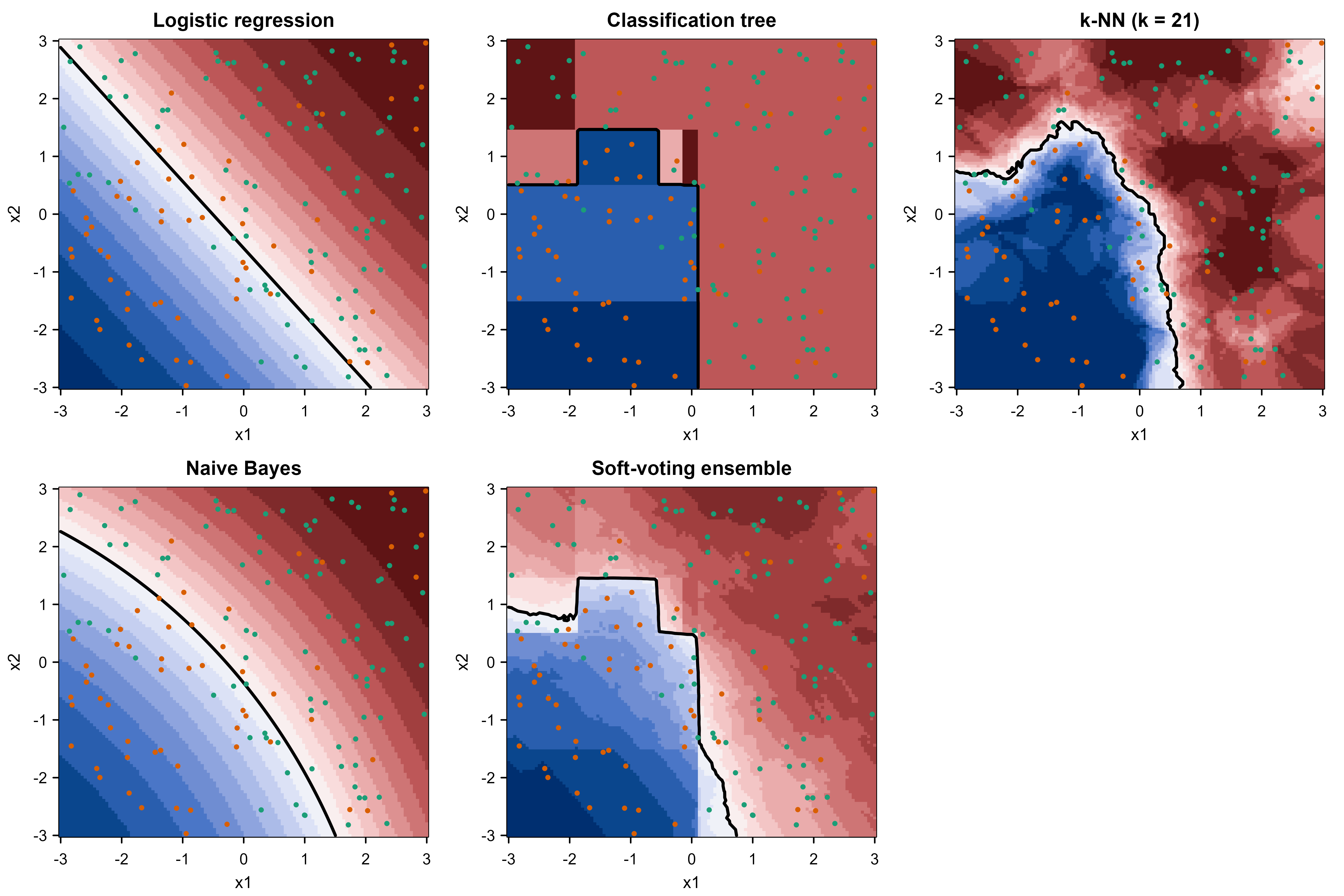
Figure 57.1 makes the decorrelation argument tangible: the members really do disagree about where the boundary lies, and the ensemble’s boundary is the consensus that survives their disagreement.
57.4 When ensembles help, and when they do not
The theory tells you exactly when to expect a gain and when not to.
When to use this
Reach for an ensemble when (1) you have several models that are each better than chance, (2) they make different mistakes (low correlation), and (3) a small, stable accuracy gain is worth extra compute and reduced interpretability. If any of these fails, the ensemble may not help.
The strongest practical lever is diversity. You manufacture it by varying the data (bagging, random subspaces), varying the algorithm (mixing model families, as in the demo above), or varying the sequence (boosting). Combining ten tuned gradient-boosted models that were all trained the same way gives far less than combining a boosted model, a random forest, a regularized linear model, and a neural net, because the latter set disagrees more. (See Chapter 12 for gradient boosting, Chapter 13 for random forests, and Chapter 15 for neural nets.)
For classification there is a quantitative counterpart to the regression variance floor, due to Breiman’s analysis of random forests. Define each member’s margin as the gap between the vote share for the true class and the largest vote share for any wrong class; the ensemble errs on a point only when this margin goes negative. Breiman bounds the generalization error of a voting ensemble by \[ \text{error} \le \frac{\bar\rho\,(1 - s^2)}{s^2}, \tag{57.3}\] where \(s\) is the mean margin (member “strength”) and \(\bar\rho\) is the mean correlation between member margins. The structure mirrors the regression result exactly: the bound shrinks as strength \(s\) rises and as correlation \(\bar\rho\) falls, and it is the ratio that matters. Adding members that are individually strong but mutually correlated raises \(\bar\rho\) and can leave the bound unchanged, the classification echo of the \(\rho v\) floor. This is the formal reason random forests randomize features: trees built on random subspaces have lower \(\bar\rho\) at a small cost in \(s\), and Equation 57.3 rewards that trade.
A few pitfalls recur often enough to call out.
Warning
Averaging strongly correlated members buys almost nothing. The variance floor is \(\rho v\); if \(\rho\) is near \(1\), you have paid for \(M\) models and kept the variance of one.
Warning
A bad member can drag down a plain average. Voting and averaging assume members are at least better than chance (the \(p > 1/2\) condition in Condorcet). Including a member that is worse than random, or one that is systematically biased in the same direction as the others, can move the ensemble the wrong way. Use weighting or stacking to suppress weak members, and validate the combination, not just the members.
Warning
Fitting combination weights (or a stacking meta-learner) on the same data used to train the members leaks information and overfits. Always weight or stack on held-out or out-of-fold predictions. This is the single most common ensemble mistake.
Two further considerations are operational rather than statistical. Ensembles cost more at training and inference time, since you must run every member, which can matter for latency-sensitive deployment. And they are harder to explain: a stakeholder can follow one decision tree but not a weighted blend of four models, so plan for interpretability tooling (Chapter 35) if explanations are required. None of these is a reason to avoid ensembles, but each is a reason to be deliberate.
A useful closing perspective: the deepest theoretical reason no single algorithm is always best is the “no free lunch” result (Wolpert and Macready, 1997). Averaged over all possible problems, every learner is equally good. Ensembles are a hedge against not knowing which inductive bias your problem rewards. By blending several biases you avoid betting the whole result on one guess about the structure of the world, which is why a well-built ensemble is so often the safe and the strong choice at once.
57.5 Further reading
- Dietterich (2000), Ensemble Methods in Machine Learning, a concise survey of why and how ensembles work, including the statistical, computational, and representational arguments for combining.
- Breiman (1996), Bagging Predictors, and Breiman (2001), Random Forests, the founding papers for the variance-reduction-by-resampling view.
- Freund and Schapire (1997), A Decision-Theoretic Generalization of On-Line Learning and an Application to Boosting, the AdaBoost paper that turns weak learners into strong ones.
- Wolpert (1992), Stacked Generalization, and Breiman (1996), Stacked Regressions, which put learned combination on a firm footing.
- Krogh and Vedelsby (1995), Neural Network Ensembles, Cross Validation, and Active Learning, the source of the ambiguity (bias-variance-diversity) decomposition.
- Ueda and Nakano (1996), Generalization Error of Ensemble Estimators, the exact bias-variance-covariance decomposition for averaged predictors.
- Hastie, Tibshirani, and Friedman (2009), The Elements of Statistical Learning, chapters on model averaging, bagging, and boosting for the unified statistical treatment.
- Zhou (2012), Ensemble Methods: Foundations and Algorithms, a book-length, modern reference covering diversity, combination rules, and advanced methods.
- Condorcet (1785), Essai sur l’application de l’analyse a la probabilite des decisions rendues a la pluralite des voix, the original jury theorem behind majority voting.