Imagine a help desk where, instead of one generalist trying to answer every question, the front desk listens to your problem and forwards you to the specialist who handles that kind of issue. The specialists never have to be good at everything; the front desk only has to be good at routing. A mixture of experts is exactly this arrangement turned into a statistical model.
More precisely, a mixture of experts (MoE) splits a prediction problem into pieces, trains a set of specialist sub-models (the experts), and learns a separate routing function (the gating network) that decides which experts handle which inputs. Instead of forcing one model to be good everywhere, you let several smaller models each be good in their own region of the input space, then combine them with input-dependent weights.
This chapter builds the idea from the ground up. We start with the intuition and the probabilistic model, derive the Expectation-Maximization (EM) algorithm that fits it, then show how the same machinery scales up to the sparse mixture of experts layers that power today’s largest language models. Along the way you will fit a working two-expert mixture in base R and see it recover a regime change that a single line cannot. By the end you should understand both the classical model and why MoE has become a standard tool for scaling modern AI.
Key idea
A mixture of experts is an ensemble whose combination weights depend on the input. The gate decides who answers, and that decision changes from one input to the next.
The idea goes back to Jacobs et al. (1991) and Jordan and Jacobs (1994), who framed it as a probabilistic model fit with an EM-like procedure. The same idea now powers some of the largest neural networks in production, where it appears as the sparse mixture of experts layer inside transformers (Chapter 38) (Shazeer et al. 2017; Fedus, Zoph, and Shazeer 2022). The modern motivation is conditional computation, the practice of activating only part of a model for each input: a model can hold a very large number of parameters but only switch on a small fraction of them per input, so the compute cost per token stays roughly fixed while capacity grows.
45.1 Where this fits in a modern ML/AI workflow
For a data scientist or ML engineer, MoE shows up in three practical situations.
Heterogeneous data with regime structure. When the relationship between predictors and target changes across regions (different customer segments, different operating regimes of a machine, piecewise dynamics), a single global model underfits. MoE lets the gate discover the regimes and assigns an expert to each.
Scaling model capacity under a compute budget. In large language models, a dense feed-forward block is replaced by many parallel expert blocks plus a router that sends each token to only the top-\(k\) experts (often \(k = 1\) or \(k = 2\)). The model can have hundreds of billions of parameters while activating only a few billion per token. This is the dominant reason MoE is discussed in 2020s AI engineering.
Ensembling with specialization. Unlike bagging (Chapter 10) or stacking where every base model sees every input, MoE weights are input-dependent. The combination is local, not global, which is closer to a learned partition of the feature space than to a uniform average.
The core distinction from a standard ensemble is that the mixture weights depend on \(x\). A stacked ensemble (see the model stacking chapter, Chapter 93) learns fixed blend weights; a mixture of experts learns weights \(g_k(x)\) that change with the input.
Intuition
Stacking asks “what is the best fixed recipe for blending these models everywhere?” A mixture of experts asks “given this input, who should I trust right now?” The second question is harder, but it is the right one when no single model is good across the whole input space.
With that motivation in place, we now write the model down precisely.
45.2 The model
The model has two parts, the experts and the gate, so we describe each in turn before combining them.
Let the input be \(x \in \mathbb{R}^p\) and the target be \(y\). We have \(K\) experts. Expert \(k\) produces a conditional distribution \(p_k(y \mid x, \theta_k)\), for example a Gaussian whose mean is a linear function of \(x\) for regression, or a softmax over classes for classification.1
The gating network produces a probability vector \(g(x) = (g_1(x), \dots, g_K(x))\) with \(g_k(x) \ge 0\) and \(\sum_k g_k(x) = 1\). You can read \(g_k(x)\) as “the share of the prediction we hand to expert \(k\) for this particular input.” The standard choice is a softmax over linear scores:
So to predict, you run every expert, ask the gate how much to weight each one for this input, and take the weighted average. The only thing left is to learn the parameters from data, which is what the next section does.
45.2.1 Fitting with EM
Fitting an MoE looks circular at first: to know which expert should handle a point we need the experts to already be trained, but to train an expert we need to know which points belong to it. EM resolves the chicken-and-egg problem by alternating soft guesses for one while holding the other fixed.
Introduce a latent indicator \(z \in \{1, \dots, K\}\) for which expert generated a given observation, with prior \(P(z = k \mid x) = g_k(x)\).2 The data log-likelihood over \(n\) observations is
This is a log of a sum, which is awkward to maximize directly, so we use Expectation-Maximization.
E-step (who is responsible?). Given current parameters, compute the responsibility of expert \(k\) for observation \(i\), which is the posterior probability that \(z_i = k\):
The responsibility \(r_{ik}\) is a soft assignment: it blends what the gate expected (the prior \(g_k\)) with how well expert \(k\) actually fit this point (the likelihood \(p_k\)). An expert that the gate favored but that fit poorly will see its responsibility shrink.
M-step (retrain given the soft assignments). Maximize the expected complete-data log-likelihood. Conveniently, this decouples into two independent pieces, one for the experts and one for the gate.
Experts. Each expert is fit by responsibility-weighted maximum likelihood. For Gaussian linear experts this is weighted least squares with weights \(r_{ik}\):
\[
\beta_k = \left( X^\top W_k X \right)^{-1} X^\top W_k y, \qquad W_k = \mathrm{diag}(r_{1k}, \dots, r_{nk}),
\]
Gate. The gating parameters maximize \(\sum_{i} \sum_{k} r_{ik} \log g_k(x_i)\), which is exactly the objective of a multinomial logistic regression with the responsibilities as soft labels. There is no closed form, so we take one or a few gradient steps per M-step. The gradient with respect to \(v_k\) is
Notice the gate gradient has the same form you see in logistic regression: the prediction error \(r_{ik} - g_k(x_i)\) times the input. The gate is simply being trained to match the responsibilities the E-step produced.
Note
EM increases the log-likelihood at every iteration and converges to a local optimum, never guaranteed to be the global one. Because experts are interchangeable, different starts can land on different (but equally good) solutions, so running several random restarts and keeping the best log-likelihood is standard practice.
We will watch this monotone increase happen in the demo below.
45.2.2 Deriving the EM updates from the complete-data likelihood
The updates above were stated; here we derive every one of them from first principles so nothing is taken on faith. The derivation is the canonical EM argument specialized to the MoE model and it makes precise why the experts and the gate decouple.
Write the latent indicator as a one-hot vector \(z_i = (z_{i1}, \dots, z_{iK})\) with \(z_{ik} = 1\) if observation \(i\) was generated by expert \(k\) and \(0\) otherwise. The complete-data likelihood for one observation factorizes into a gate term and an expert term because, conditional on \(x_i\), the model first draws the expert from \(g(x_i)\) and then draws \(y_i\) from that expert:
The two bracketed terms involve disjoint parameter blocks (\(v_k\) in the first, \(\theta_k\) in the second), which is the structural reason the M-step will split into an independent gate problem and independent expert problems.
E-step as the tight variational bound. EM maximizes \(\ell(\Theta)\) indirectly through the auxiliary function \(Q(\Theta \mid \Theta^{(t)}) = \mathbb{E}\big[ \ell_c(\Theta) \mid x, y, \Theta^{(t)} \big]\). Since \(\ell_c\) is linear in the \(z_{ik}\), the expectation only needs \(\mathbb{E}[z_{ik} \mid x_i, y_i, \Theta^{(t)}] = P(z_i = k \mid x_i, y_i, \Theta^{(t)}) = r_{ik}\). By Bayes’ rule, with prior \(g_k(x_i)\) and likelihood \(p_k(y_i \mid x_i, \theta_k)\),
M-step for the experts. Each expert appears in exactly one summand of \(Q_{\text{experts}}\), so we maximize each separately. For the Gaussian linear expert, dropping constants,
In matrix form with \(W_k = \mathrm{diag}(r_{1k}, \dots, r_{nk})\) these are the weighted normal equations \(X^\top W_k X \, \beta_k = X^\top W_k y\), whose solution is the responsibility-weighted least squares estimator
\[
\beta_k = \big( X^\top W_k X \big)^{-1} X^\top W_k y ,
\]
confirming the update stated above. Differentiating \(Q_k\) with respect to \(\sigma_k^2\),
the responsibility-weighted residual variance. The denominator \(\sum_i r_{ik}\) is the effective sample size of expert \(k\), which explains the degeneracy warning later: if an expert collects almost no responsibility, this denominator vanishes and \(\sigma_k^2\) can collapse to zero.
M-step for the gate. The gate maximizes \(Q_{\text{gate}}(\{v_k\}) = \sum_i \sum_k r_{ik} \log g_k(x_i)\) with \(g_k\) the softmax. Using the standard softmax Jacobian \(\partial \log g_j(x_i) / \partial v_k = (\mathbb{1}[j = k] - g_k(x_i))\, x_i\),
which recovers the gate gradient stated earlier and shows it is precisely the score of a multinomial logistic regression with the soft targets \(r_{ik}\). Because \(g_k\) is nonlinear in \(v_k\), there is no closed form, so we take gradient (or a few Newton/IRLS) steps; doing a partial maximization here is the generalized EM variant, which still increases \(\ell\) at each iteration.
Why the likelihood never decreases
For any distribution \(q_i(k)\), Jensen’s inequality gives the evidence lower bound \(\log \sum_k g_k(x_i) p_k(y_i) \ge \sum_k q_i(k) \log \tfrac{g_k(x_i) p_k(y_i)}{q_i(k)}\), with equality exactly when \(q_i(k) = r_{ik}\). The E-step sets \(q_i = r_i\) to make the bound tight at \(\Theta^{(t)}\); the M-step raises the bound. Since the bound touches \(\ell\) at \(\Theta^{(t)}\) and lies below it everywhere, raising the bound raises \(\ell\): \(\ell(\Theta^{(t+1)}) \ge \ell(\Theta^{(t)})\). This is the monotonicity the demo verifies numerically.
45.2.3 Theoretical properties and connections
A few facts sharpen when MoE works, how fast EM gets there, and how it relates to neighboring methods.
Identifiability and label switching. The mixture density is invariant to permuting expert indices, so the parameter \(\Theta\) is identifiable only up to relabeling, a \(K!\)-fold symmetry. This is harmless for prediction (the predictive density Equation 45.1 is permutation invariant) but means individual coordinates of \(\Theta\) have no fixed meaning, which is why expert indices must not be interpreted as stable across restarts. A second, subtler nonidentifiability arises when an expert is empty (\(g_k \equiv 0\)) or duplicated; at such points the Fisher information is singular, so standard asymptotic normality of the MLE fails and likelihood-ratio tests for the number of experts do not have the usual \(\chi^2\) limit. This is the MoE instance of the general theory of singular learning in mixtures.
Convergence rate of EM. EM is a first-order method: near a local optimum \(\Theta^\star\) the error contracts linearly, \[
\| \Theta^{(t+1)} - \Theta^\star \| \approx \rho \, \| \Theta^{(t)} - \Theta^\star \|, \qquad \rho = \lambda_{\max}\!\big( I_{\text{mis}} I_{\text{com}}^{-1} \big),
\] where the rate \(\rho \in [0,1)\) is the largest eigenvalue of the ratio of the missing information (about \(z\)) to the complete information. Well separated experts give little missing information, so \(\rho \approx 0\) and EM converges in a handful of iterations; heavily overlapping experts give \(\rho \to 1\) and EM crawls. This is why spreading the initial expert slopes apart (as the demo does) matters: it reduces the initial overlap and the missing information.
Bias, variance, and the effect of \(K\). Increasing \(K\) lowers approximation bias because a piecewise model can match a more intricate conditional mean, but it raises variance: each expert is fit on an effective sample size \(\sum_i r_{ik}\) that shrinks roughly like \(n/K\), and the gate gains \(p(K-1)\) parameters. The model selects \(K\) like any complexity parameter, by penalized likelihood. With \(d_K = K(2p+1) - p\) free parameters (each expert contributes \(\beta_k \in \mathbb{R}^p\) and \(\sigma_k^2\), the gate contributes \(K-1\) identifiable score vectors in \(\mathbb{R}^p\)), the Bayesian information criterion is \[
\mathrm{BIC}(K) = -2\,\ell(\hat\Theta_K) + d_K \log n ,
\] chosen as the smallest BIC over a grid of \(K\); the singular geometry above means BIC is a practical guide rather than a theorem here, so confirm with held-out likelihood.
Connection to hierarchical mixtures and to soft trees. Stacking gates recursively gives the hierarchical mixture of experts of Jordan and Jacobs (1994): a tree of gates routes an input down to a leaf expert, and the path probability is the product of the gate probabilities along the route. A standard decision tree (Chapter 8) is the hard limit of an HME in which every gate outputs \(0\) or \(1\), so an HME is a smoothed, EM-trainable relaxation of a regression tree. The dense MoE in this chapter is the depth-one case.
Connection to the softmax and to attention. A single softmax-gated MoE with one expert per class reduces to multinomial logistic regression, so MoE strictly generalizes the softmax classifier by attaching a full model to each “class.” The input-dependent convex combination \(\sum_k g_k(x) f_k(x)\) also has the same algebraic form as an attention readout (Chapter 38), with the gate playing the role of attention weights over a fixed set of value vectors; the difference is that the gate is normalized over experts rather than over positions.
45.3 Sparse mixture of experts and top-k routing
So far we have a clean classical model. The reason MoE is everywhere in modern AI, though, is a single change that makes it scale, and that is the subject of this section.
The model above is dense: every expert is evaluated for every input, then combined. That is fine for \(K = 2\) or \(K = 10\), but it does not scale to thousands of experts because cost grows linearly in \(K\).
The sparse variant keeps the same gating scores but evaluates only the top-\(k\) experts per input.3 Let \(\mathrm{TopK}(s, k)\) keep the \(k\) largest gating logits \(s_j = v_j^\top x\) and set the rest to \(-\infty\) before the softmax:
Only the selected experts run, so per-input compute depends on \(k\), not on \(K\). Adding more experts increases capacity (total parameters) without increasing per-input FLOPs. This is the conditional computation property that makes trillion-parameter language models feasible (Fedus, Zoph, and Shazeer 2022).
Key idea
Sparsity decouples capacity from cost. A dense model that doubles its parameters doubles its compute per input. A sparse MoE can multiply its parameters many times over while the work done per input barely moves, because each input still only touches \(k\) experts.
45.3.1 Load balancing
Sparse routing has a failure mode: the gate can collapse onto a few popular experts, leaving others untrained, which wastes capacity and unbalances hardware utilization. This is a real and common problem, not a theoretical worry, so production systems always guard against it. The standard fix is an auxiliary load-balancing loss added to the training objective. With \(f_k\) the fraction of inputs in a batch routed to expert \(k\) and \(P_k\) the average gate probability assigned to expert \(k\), a common penalty (Shazeer et al. 2017; Fedus, Zoph, and Shazeer 2022) is
which is minimized when routing is uniform. Other practical devices include a per-expert capacity limit (drop or overflow tokens beyond a cap) and adding noise to the gating logits during training to encourage exploration.
To see why this particular product is the right penalty, note two things. First, by the constraint \(\sum_k f_k = \sum_k P_k = 1\), the dot product \(\sum_k f_k P_k\) is the expectation of a uniform-vs-actual comparison. Treating \(f\) and \(P\) as nearly aligned (the gate that routes a token also assigns it high probability), \(\sum_k f_k P_k \approx \sum_k f_k^2 = \tfrac{1}{K} + \mathrm{Var}_k(K f_k)/K\) up to the floor \(1/K\) attained only at the uniform routing \(f_k = 1/K\), so minimizing \(L_{\text{balance}}\) minimizes the variance of the load across experts. The factor of \(K\) makes the minimum value \(\alpha\) independent of the expert count, so \(\alpha\) transfers across model sizes. Second, the penalty is constructed to be differentiable through \(P_k\) even though the load \(f_k\) comes from a hard, non-differentiable top-\(k\) selection: gradients flow through the soft probabilities \(P_k\) while \(f_k\) acts as a (detached) coefficient, which is exactly what lets the router learn to spread traffic by gradient descent despite the discrete routing decision.
Warning
If you train a sparse MoE without a load-balancing term, expect a few experts to win all the traffic while the rest stay at their random initialization. The auxiliary loss is not optional in practice.
45.3.2 Dense vs sparse mixture
Table 45.1 summarizes the trade-off between the two flavors so you can pick the right one for the job.
Table 45.1: Comparison of dense and sparse top-\(k\) mixtures of experts across compute cost, scale, training stability, and routing.
Property
Dense MoE
Sparse MoE (top-\(k\))
Experts evaluated per input
all \(K\)
only \(k \ll K\)
Per-input compute
grows with \(K\)
roughly fixed in \(K\)
Total parameters used per input
all
a fraction
Typical scale
small \(K\) (2 to tens)
large \(K\) (tens to thousands)
Training stability
straightforward EM or gradient
needs load balancing, capacity limits
Main use
regime/segment modeling
scaling LLM capacity
Routing
soft weights
hard top-\(k\) selection
45.4 MoE compared to related methods
It helps to place MoE next to the other ensemble methods in this book. Table 45.2 lays out the comparison, and the single column that sets MoE apart is the last one: whether the combination weights are allowed to depend on the input.
Table 45.2: How a mixture of experts compares to bagging, stacking, and boosting, with input-dependent combination weights as the distinguishing feature.
Method
Combination weights
Specialization
Weights depend on \(x\)?
Bagging / random forest
uniform average
none (same task)
no
Stacking
learned, fixed
mild
no
Boosting
sequential, additive
residual-focused
no (additive)
Mixture of experts
learned gate
strong, by region
yes
Sparse MoE layer
learned top-\(k\) gate
strong, by token
yes (hard)
45.5 Runnable demo: two-expert mixture on piecewise data
Enough theory. Let us watch the EM algorithm actually discover a hidden partition of the data with no labels telling it where the boundary is.
We simulate data where the slope of \(y\) in \(x\) flips sign at \(x = 0\). A single linear regression is hopeless here, because the best single line through a V-shaped cloud is roughly flat, but two linear experts plus a softmax gate can recover the two regimes. We fit with the EM updates derived above, all in base R so nothing is hidden inside a package.
When to use this
A worked-from-scratch fit like this one is exactly the case MoE was designed for, a relationship whose shape changes across regions of the input. If your relationship is globally smooth, reach for a GAM or boosted trees instead (see the guidance section at the end).
Show code
set.seed(1301)# simulate piecewise-linear data with a regime change at x = 0n<-400x<-runif(n, -3, 3)# regime A (x < 0): negative slope; regime B (x >= 0): positive slopemu<-ifelse(x<0, 2-1.6*x, 2+1.6*x)y<-mu+rnorm(n, sd =0.6)X<-cbind(1, x)# design matrix for experts and gateK<-2# number of experts
Show code
# Gaussian density helperdnorm_safe<-function(y, mu, s2){dnorm(y, mean =mu, sd =sqrt(pmax(s2, 1e-8)))}softmax_rows<-function(S){S<-S-apply(S, 1, max)# numerical stabilityE<-exp(S)E/rowSums(E)}fit_moe<-function(X, y, K=2, iters=100, gate_steps=5,gate_lr=0.05, seed=1){set.seed(seed)n<-nrow(X); p<-ncol(X)# init experts by spreading their slopes apart so EM does not start in a# symmetric trap where every expert claims equal responsibility everywherebeta_ols<-as.numeric(solve(t(X)%*%X, t(X)%*%y))Beta<-matrix(beta_ols, nrow =p, ncol =K)Beta[p, ]<-beta_ols[p]+seq(-3, 3, length.out =K)# vary the slope rowBeta<-Beta+matrix(rnorm(p*K, sd =0.3), p, K)s2<-rep(var(y), K)V<-matrix(rnorm(p*K, sd =0.1), nrow =p, ncol =K)# small random gate initll_trace<-numeric(iters)for(itin1:iters){# gate probabilitiesG<-softmax_rows(X%*%V)# n x K# expert means and densitiesM<-X%*%Beta# n x KD<-sapply(1:K, function(k)dnorm_safe(y, M[, k], s2[k]))# n x K# E-step: responsibilitiesnum<-G*Dden<-rowSums(num)+1e-12R<-num/denll_trace[it]<-sum(log(den))# M-step experts: weighted least squares per expertfor(kin1:K){w<-R[, k]XtWX<-t(X*w)%*%XXtWy<-t(X*w)%*%yBeta[, k]<-solve(XtWX+diag(1e-8, p), XtWy)resid<-y-X%*%Beta[, k]s2[k]<-sum(w*resid^2)/(sum(w)+1e-12)}# M-step gate: a few gradient ascent steps on sum_i sum_k R_ik log G_ikfor(gin1:gate_steps){G<-softmax_rows(X%*%V)grad<-t(X)%*%(R-G)# p x KV<-V+gate_lr*grad}}list(Beta =Beta, s2 =s2, V =V, R =R, G =softmax_rows(X%*%V), ll =ll_trace)}fit<-fit_moe(X, y, K =2, iters =150, gate_steps =8, gate_lr =0.03, seed =7)# recovered expert slopes (one should be near -1.6, the other near +1.6)round(fit$Beta, 3)#> [,1] [,2]#> [1,] 2.003 2.014#> [2,] 1.583 -1.596
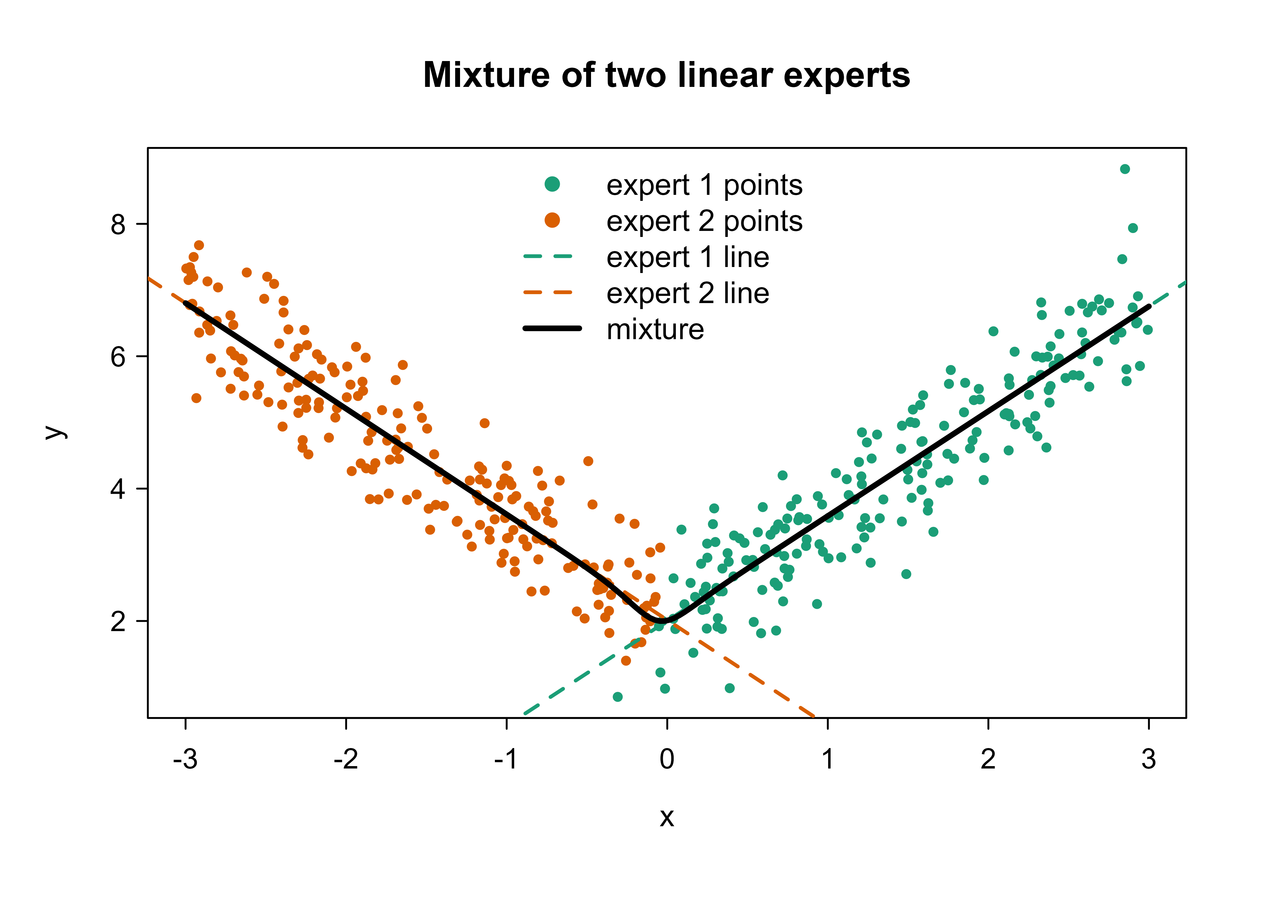
Read the output as two columns, one per expert. One expert recovered a slope near \(-1.6\) and the other near \(+1.6\), which are exactly the two slopes we built into the simulation, even though the fit was never told where the regime boundary was. The gate learned a soft boundary near \(x = 0\) on its own. Figure 45.1 plots the data colored by which expert claims responsibility, overlays each expert’s fitted line, and shows the mixture prediction.
Show code
assign<-ifelse(fit$R[, 1]>=fit$R[, 2], 1L, 2L)# gate-weighted mixture prediction on a gridxg<-seq(-3, 3, length.out =200)Xg<-cbind(1, xg)Gg<-softmax_rows(Xg%*%fit$V)Mg<-Xg%*%fit$Betamix<-rowSums(Gg*Mg)plot(x, y, col =ifelse(assign==1, "#1b9e77", "#d95f02"), pch =19, cex =0.6, xlab ="x", ylab ="y", main ="Mixture of two linear experts")abline(a =fit$Beta[1, 1], b =fit$Beta[2, 1], col ="#1b9e77", lwd =2, lty =2)abline(a =fit$Beta[1, 2], b =fit$Beta[2, 2], col ="#d95f02", lwd =2, lty =2)lines(xg, mix, col ="black", lwd =3)legend("top", bty ="n", legend =c("expert 1 points", "expert 2 points","expert 1 line", "expert 2 line", "mixture"), col =c("#1b9e77", "#d95f02", "#1b9e77", "#d95f02", "black"), pch =c(19, 19, NA, NA, NA), lty =c(NA, NA, 2, 2, 1), lwd =c(NA, NA, 2, 2, 3))
Figure 45.1: Two-expert mixture on piecewise data. Points are colored by the expert with higher responsibility, the dashed lines are the two linear experts, and the solid line is the gate-weighted mixture prediction.
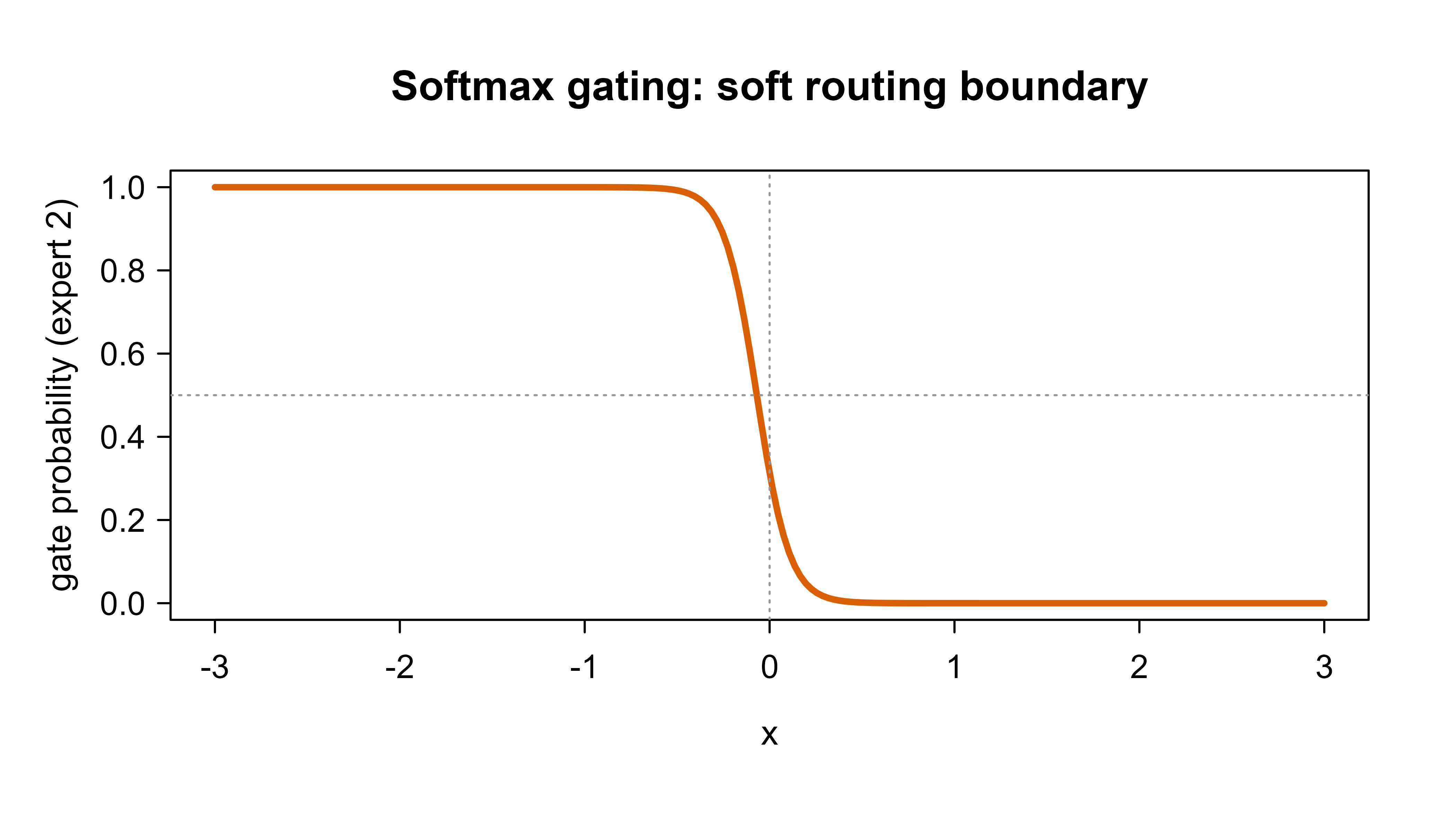
We can also check that the gate behaves like a learned soft router: the probability of expert 2 should rise as \(x\) increases. Figure 45.2 plots that learned gating probability across the input range.
Show code
plot(xg, Gg[, 2], type ="l", lwd =3, col ="#d95f02", ylim =c(0, 1), xlab ="x", ylab ="gate probability (expert 2)", main ="Softmax gating: soft routing boundary")abline(v =0, col ="grey60", lty =3)abline(h =0.5, col ="grey60", lty =3)
Figure 45.2: Learned gating probability for expert 2 as a function of x. The softmax gate forms a soft routing boundary near the regime change.
Show code
# EM should increase the log-likelihood monotonically (up to gate sub-steps)ll<-fit$llcat("first 3 log-likelihoods:", round(head(ll, 3), 1), "\n")#> first 3 log-likelihoods: -2467.4 -1452.2 -694.1cat("last 3 log-likelihoods :", round(tail(ll, 3), 1), "\n")#> last 3 log-likelihoods : -359.5 -359.5 -359.5cat("monotone non-decreasing:",all(diff(ll)>-1e-6), "\n")#> monotone non-decreasing: TRUE
The log-likelihood climbs from a poor start and flattens out, and the final check confirms it never went down (allowing a tiny tolerance for the gate’s inner gradient steps). That monotone increase is the theoretical guarantee of EM made visible.
We can also verify the tight-bound identity behind the monotonicity proof: at the responsibilities \(r_{ik}\), the evidence lower bound equals the exact log-likelihood, so their difference is zero up to numerical error.
Show code
# recompute responsibilities at the fitted parametersG<-fit$GM<-X%*%fit$BetaD<-sapply(1:K, function(k)dnorm_safe(y, M[, k], fit$s2[k]))num<-G*DR<-num/(rowSums(num)+1e-300)ll_exact<-sum(log(rowSums(G*D)))# log sum_k g_k p_kelbo<-sum(R*log((G*D)/(R+1e-300)))# ELBO at q = rc(loglik =round(ll_exact, 4), elbo =round(elbo, 4), gap =signif(ll_exact-elbo, 3))# should be ~ 0#> loglik elbo gap #> -359.5354 -359.5354 0.0000
The gap is essentially zero, confirming that the E-step makes Jensen’s bound tight, which is precisely why each M-step increase carries over to the true log-likelihood.
A single global linear fit for comparison makes the gain concrete:
Show code
ols<-lm(y~x)mse_ols<-mean(residuals(ols)^2)# mixture training MSE using the gate-weighted mean at each pointG_full<-fit$GM_full<-X%*%fit$Betayhat_moe<-rowSums(G_full*M_full)mse_moe<-mean((y-yhat_moe)^2)c(ols_mse =round(mse_ols, 3), moe_mse =round(mse_moe, 3))#> ols_mse moe_mse #> 2.329 0.354
The mixture cuts training error substantially because it fits each regime with its own line rather than averaging the two slopes into a flat compromise.
45.6 Sketch of top-k routing in base R
The dense demo above evaluated both experts everywhere. To make the sparse idea concrete without a deep learning stack, here is a tiny top-\(k\) router over gating logits. With \(K = 2\) and \(k = 1\) it becomes hard assignment, where each input picks exactly one expert; the same code generalizes to many experts.
Show code
top_k_gate<-function(S, k){# S: n x K matrix of gating logits; return sparse normalized weightsn<-nrow(S); K<-ncol(S)W<-matrix(0, n, K)for(iin1:n){keep<-order(S[i, ], decreasing =TRUE)[1:k]e<-exp(S[i, keep]-max(S[i, keep]))W[i, keep]<-e/sum(e)}W}S<-X%*%fit$VW1<-top_k_gate(S, k =1)# hard routing: each row picks one expert# fraction of inputs routed to each expert (load), should be away from 0 and 1round(colMeans(W1>0), 3)#> [1] 0.495 0.505
Here the load is close to a 50/50 split, which is what we want. In a real sparse MoE you would add the load-balancing penalty \(L_{\text{balance}}\) from above so neither expert is starved, and a capacity cap so no expert is overloaded within a batch.
45.7 A note on the deep learning version
In a transformer (Chapter 38), the experts are feed-forward sub-networks and the gate is a small linear layer applied per token. The code below is the idiomatic Keras shape of a single sparse MoE feed-forward layer. It is kept eval=FALSE because it needs a configured deep learning backend (Keras and its TensorFlow backend), but it is correct, runnable code.
Tip
Even in the deep learning version, the two moving parts are the same ones we derived classically: a gate that scores experts and a weighted combination of expert outputs. The novelty is engineering (sparsity, capacity, distributing experts across devices), not a new statistical idea.
Show code
library(keras)# A simplified top-1 routed MoE feed-forward layer for one token embedding.# d_model: embedding size, d_ff: expert hidden size, num_experts: K.moe_ffn<-function(x, d_model=256L, d_ff=1024L, num_experts=8L){# gate logits per token, then softmax over expertsgate_logits<-layer_dense(x, units =num_experts)# (batch, K)gate<-layer_activation_softmax(gate_logits)# (batch, K)# build K independent expert FFNs and stack their outputsexpert_outs<-lapply(seq_len(num_experts), function(k){h<-layer_dense(x, units =d_ff, activation ="gelu")layer_dense(h, units =d_model)# (batch, d_model)})stacked<-k_stack(expert_outs, axis =2L)# (batch, K, d_model)# weighted combination by gate (dense form shown; sparse would gather top-k)w<-k_expand_dims(gate, axis =-1L)# (batch, K, 1)k_sum(stacked*w, axis =2L)# (batch, d_model)}# Auxiliary load-balancing loss to discourage expert collapse.load_balance_loss<-function(gate, alpha=0.01){importance<-k_mean(gate, axis =1L)# P_kload<-k_mean(k_cast(gate>0, "float32"), axis =1L)# f_kK<-k_int_shape(gate)[[2]]alpha*K*k_sum(importance*load)}
45.8 Practical guidance, pitfalls, and when to use it
A mixture of experts is powerful but has sharp edges, so this section collects what tends to go right and wrong in practice.
When MoE helps.
The conditional mean or class boundary changes shape across regions of the input space, and you can plausibly describe those regions from the features.
You want to scale model capacity but keep per-input inference cost bounded (the sparse, deep learning case).
You have enough data per region. Each expert effectively trains on a fraction of the data, so MoE is data-hungry relative to a single model.
When to prefer something else.
If the relationship is globally smooth, a GAM (see the generalized additive models chapter, Chapter 6) or a gradient-boosted tree (see the boosting chapter, Chapter 11) is simpler and usually stronger.
With little data, the latent assignment is unstable and the gate overfits; a single regularized model is safer.
Pitfalls.
Local optima. EM converges to a local maximum. Run several random restarts and keep the best log-likelihood. The demo uses a fixed seed for reproducibility, but in practice vary it.
Degenerate experts. An expert can grab almost no responsibility and have its variance collapse toward zero, inflating its density. Floor the variance (the pmax(s2, 1e-8) above) and consider pruning or reinitializing dead experts.
Gate collapse in the sparse case. Without a load-balancing term, the router sends everything to a few experts. Always add the auxiliary loss and a capacity limit when training sparse MoE.
Identifiability. Experts are exchangeable, so the labels (which expert is “expert 1”) are arbitrary and can swap across restarts. Do not interpret expert indices as fixed.
Choosing \(K\). Treat the number of experts as a hyperparameter. Use a validation metric or an information criterion; more experts is not automatically better and raises overfitting risk in the dense case.
Routing instability. Hard top-\(k\) routing has discrete decisions that can flip during training; noisy gating and a small temperature on the gate logits help smooth optimization.
Operational notes for the sparse case. Expert parallelism places different experts on different devices, so the all-to-all communication that shuffles tokens to their chosen experts often dominates wall-clock time, not the matrix multiplies. Capacity factor, batch size, and the number of experts per device are the knobs that matter most for throughput.
To summarize the whole chapter in one line: a mixture of experts is an ensemble whose weights depend on the input, fit classically by EM and scaled in deep learning by routing each input to only its top few experts. The same two ideas, a gate and specialized experts, carry you from a two-line toy model to trillion-parameter language models.
45.9 Further reading
The references below trace the arc from the original statistical formulation to the modern sparse layers.
Jacobs, Jordan, Nowlan, and Hinton (1991), “Adaptive mixtures of local experts.” The original formulation.
Jordan and Jacobs (1994), “Hierarchical mixtures of experts and the EM algorithm.” The EM treatment and the hierarchical (tree-structured) gate.
Shazeer et al. (2017), “Outrageously large neural networks: the sparsely-gated mixture-of-experts layer.” Top-\(k\) routing and load balancing at scale.
Fedus, Zoph, and Shazeer (2022), “Switch Transformers: scaling to trillion parameter models with simple and efficient sparsity.” Top-1 routing, capacity factors, and large-scale training practice.
Bishop (2006), Pattern Recognition and Machine Learning, chapter on mixture models and EM, for the probabilistic background.
Fedus, William, Barret Zoph, and Noam Shazeer. 2022. “Switch Transformers: Scaling to Trillion Parameter Models with Simple and Efficient Sparsity.”Journal of Machine Learning Research 23 (120): 1–39.
Jacobs, Robert A., Michael I. Jordan, Steven J. Nowlan, and Geoffrey E. Hinton. 1991. “Adaptive Mixtures of Local Experts.”Neural Computation 3 (1): 79–87.
Jordan, Michael I., and Robert A. Jacobs. 1994. “Hierarchical Mixtures of Experts and the EM Algorithm.”Neural Computation 6 (2): 181–214.
Shazeer, Noam, Azalia Mirhoseini, Krzysztof Maziarz, Andy Davis, Quoc Le, Geoffrey Hinton, and Jeff Dean. 2017. “Outrageously Large Neural Networks: The Sparsely-Gated Mixture-of-Experts Layer.” In International Conference on Learning Representations (ICLR).
Nothing forces the experts to be simple. In the classical statistical literature they are usually linear or generalized linear models because that keeps the M-step in closed form, but in deep learning each expert is itself a small neural network.↩︎
We never observe \(z\); it is a modeling fiction that says “imagine each point really was produced by one specific expert.” Treating \(z\) as a hidden variable is the trick that turns a hard direct optimization into the easy two-step EM loop.↩︎
Here \(k\) (lowercase) is the number of experts you keep per input, typically 1 or 2, while \(K\) (uppercase) is the total number of experts, which can be in the thousands. Do not confuse the two.↩︎
Source Code
# Mixture of Experts and Conditional Computation {#sec-mixture-of-experts}```{r}#| include: falsesource("_common.R")```Imagine a help desk where, instead of one generalist trying to answer every question, the front desk listens to your problem and forwards you to the specialist who handles that kind of issue. The specialists never have to be good at everything; the front desk only has to be good at routing. A mixture of experts is exactly this arrangement turned into a statistical model.More precisely, a mixture of experts (MoE) splits a prediction problem into pieces, trains a set of specialist sub-models (the experts), and learns a separate routing function (the gating network) that decides which experts handle which inputs. Instead of forcing one model to be good everywhere, you let several smaller models each be good in their own region of the input space, then combine them with input-dependent weights.This chapter builds the idea from the ground up. We start with the intuition and the probabilistic model, derive the Expectation-Maximization (EM) algorithm that fits it, then show how the same machinery scales up to the *sparse* mixture of experts layers that power today's largest language models. Along the way you will fit a working two-expert mixture in base R and see it recover a regime change that a single line cannot. By the end you should understand both the classical model and why MoE has become a standard tool for scaling modern AI.::: {.callout-important title="Key idea"}A mixture of experts is an ensemble whose combination weights depend on the input. The gate decides *who answers*, and that decision changes from one input to the next.:::The idea goes back to @jacobs1991 and @jordan1994, who framed it as a probabilistic model fit with an EM-like procedure. The same idea now powers some of the largest neural networks in production, where it appears as the *sparse* mixture of experts layer inside transformers (@sec-transformers) [@shazeer2017; @fedus2022]. The modern motivation is *conditional computation*, the practice of activating only part of a model for each input: a model can hold a very large number of parameters but only switch on a small fraction of them per input, so the compute cost per token stays roughly fixed while capacity grows.## Where this fits in a modern ML/AI workflowFor a data scientist or ML engineer, MoE shows up in three practical situations.1. Heterogeneous data with regime structure. When the relationship between predictors and target changes across regions (different customer segments, different operating regimes of a machine, piecewise dynamics), a single global model underfits. MoE lets the gate discover the regimes and assigns an expert to each.2. Scaling model capacity under a compute budget. In large language models, a dense feed-forward block is replaced by many parallel expert blocks plus a router that sends each token to only the top-$k$ experts (often $k = 1$ or $k = 2$). The model can have hundreds of billions of parameters while activating only a few billion per token. This is the dominant reason MoE is discussed in 2020s AI engineering.3. Ensembling with specialization. Unlike bagging (@sec-bagging) or stacking where every base model sees every input, MoE weights are input-dependent. The combination is local, not global, which is closer to a learned partition of the feature space than to a uniform average.The core distinction from a standard ensemble is that the mixture weights depend on $x$. A stacked ensemble (see the model stacking chapter, @sec-model-stacking) learns fixed blend weights; a mixture of experts learns weights $g_k(x)$ that change with the input.::: {.callout-tip title="Intuition"}Stacking asks "what is the best fixed recipe for blending these models everywhere?" A mixture of experts asks "given *this* input, who should I trust right now?" The second question is harder, but it is the right one when no single model is good across the whole input space.:::With that motivation in place, we now write the model down precisely.## The modelThe model has two parts, the experts and the gate, so we describe each in turn before combining them.Let the input be $x \in \mathbb{R}^p$ and the target be $y$. We have $K$ experts. Expert $k$ produces a conditional distribution $p_k(y \mid x, \theta_k)$, for example a Gaussian whose mean is a linear function of $x$ for regression, or a softmax over classes for classification.^[Nothing forces the experts to be simple. In the classical statistical literature they are usually linear or generalized linear models because that keeps the M-step in closed form, but in deep learning each expert is itself a small neural network.]The gating network produces a probability vector $g(x) = (g_1(x), \dots, g_K(x))$ with $g_k(x) \ge 0$ and $\sum_k g_k(x) = 1$. You can read $g_k(x)$ as "the share of the prediction we hand to expert $k$ for this particular input." The standard choice is a softmax over linear scores:$$g_k(x) = \frac{\exp(v_k^\top x)}{\sum_{j=1}^{K} \exp(v_j^\top x)},$$where $v_k \in \mathbb{R}^p$ are the gating parameters (include a 1 in $x$ for an intercept).The mixture density is the gate-weighted sum of the expert densities:$$p(y \mid x, \Theta) = \sum_{k=1}^{K} g_k(x) \, p_k(y \mid x, \theta_k),$$ {#eq-mixture-of-experts-density}with $\Theta = \{v_k, \theta_k\}_{k=1}^K$. For a regression expert with Gaussian noise,$$p_k(y \mid x, \theta_k) = \mathcal{N}\!\left(y \,;\, \beta_k^\top x, \, \sigma_k^2\right).$$The predicted mean is then the gate-weighted combination of expert means:$$\mathbb{E}[y \mid x] = \sum_{k=1}^{K} g_k(x) \, \beta_k^\top x .$$So to predict, you run every expert, ask the gate how much to weight each one for this input, and take the weighted average. The only thing left is to learn the parameters from data, which is what the next section does.### Fitting with EMFitting an MoE looks circular at first: to know which expert should handle a point we need the experts to already be trained, but to train an expert we need to know which points belong to it. EM resolves the chicken-and-egg problem by alternating soft guesses for one while holding the other fixed.Introduce a latent indicator $z \in \{1, \dots, K\}$ for which expert generated a given observation, with prior $P(z = k \mid x) = g_k(x)$.^[We never observe $z$; it is a modeling fiction that says "imagine each point really was produced by one specific expert." Treating $z$ as a hidden variable is the trick that turns a hard direct optimization into the easy two-step EM loop.] The data log-likelihood over $n$ observations is$$\ell(\Theta) = \sum_{i=1}^{n} \log \sum_{k=1}^{K} g_k(x_i) \, p_k(y_i \mid x_i, \theta_k).$$This is a log of a sum, which is awkward to maximize directly, so we use Expectation-Maximization.E-step (who is responsible?). Given current parameters, compute the responsibility of expert $k$ for observation $i$, which is the posterior probability that $z_i = k$:$$r_{ik} = P(z_i = k \mid x_i, y_i) = \frac{g_k(x_i) \, p_k(y_i \mid x_i, \theta_k)}{\sum_{j=1}^{K} g_j(x_i) \, p_j(y_i \mid x_i, \theta_j)} .$$The responsibility $r_{ik}$ is a soft assignment: it blends what the gate expected (the prior $g_k$) with how well expert $k$ actually fit this point (the likelihood $p_k$). An expert that the gate favored but that fit poorly will see its responsibility shrink.M-step (retrain given the soft assignments). Maximize the expected complete-data log-likelihood. Conveniently, this decouples into two independent pieces, one for the experts and one for the gate.*Experts.* Each expert is fit by responsibility-weighted maximum likelihood. For Gaussian linear experts this is weighted least squares with weights $r_{ik}$:$$\beta_k = \left( X^\top W_k X \right)^{-1} X^\top W_k y, \qquad W_k = \mathrm{diag}(r_{1k}, \dots, r_{nk}),$$and the variance update$$\sigma_k^2 = \frac{\sum_{i} r_{ik} (y_i - \beta_k^\top x_i)^2}{\sum_{i} r_{ik}} .$$*Gate.* The gating parameters maximize $\sum_{i} \sum_{k} r_{ik} \log g_k(x_i)$, which is exactly the objective of a multinomial logistic regression with the responsibilities as soft labels. There is no closed form, so we take one or a few gradient steps per M-step. The gradient with respect to $v_k$ is$$\frac{\partial}{\partial v_k} \sum_i \sum_j r_{ij} \log g_j(x_i) = \sum_{i} \left( r_{ik} - g_k(x_i) \right) x_i .$$Notice the gate gradient has the same form you see in logistic regression: the prediction error $r_{ik} - g_k(x_i)$ times the input. The gate is simply being trained to match the responsibilities the E-step produced.::: {.callout-note}EM increases the log-likelihood at every iteration and converges to a *local* optimum, never guaranteed to be the global one. Because experts are interchangeable, different starts can land on different (but equally good) solutions, so running several random restarts and keeping the best log-likelihood is standard practice.:::We will watch this monotone increase happen in the demo below.### Deriving the EM updates from the complete-data likelihoodThe updates above were stated; here we derive every one of them from first principles so nothing is taken on faith. The derivation is the canonical EM argument specialized to the MoE model and it makes precise why the experts and the gate decouple.Write the latent indicator as a one-hot vector $z_i = (z_{i1}, \dots, z_{iK})$ with $z_{ik} = 1$ if observation $i$ was generated by expert $k$ and $0$ otherwise. The complete-data likelihood for one observation factorizes into a gate term and an expert term because, conditional on $x_i$, the model first draws the expert from $g(x_i)$ and then draws $y_i$ from that expert:$$p(y_i, z_i \mid x_i, \Theta) = \prod_{k=1}^{K} \big[ g_k(x_i) \, p_k(y_i \mid x_i, \theta_k) \big]^{z_{ik}} .$$Taking logs and summing over the sample gives the complete-data log-likelihood$$\ell_c(\Theta) = \sum_{i=1}^{n} \sum_{k=1}^{K} z_{ik} \Big[ \log g_k(x_i) + \log p_k(y_i \mid x_i, \theta_k) \Big] .$$ {#eq-mixture-of-experts-complete-ll}The two bracketed terms involve disjoint parameter blocks ($v_k$ in the first, $\theta_k$ in the second), which is the structural reason the M-step will split into an independent gate problem and independent expert problems.**E-step as the tight variational bound.** EM maximizes $\ell(\Theta)$ indirectly through the auxiliary function $Q(\Theta \mid \Theta^{(t)}) = \mathbb{E}\big[ \ell_c(\Theta) \mid x, y, \Theta^{(t)} \big]$. Since $\ell_c$ is linear in the $z_{ik}$, the expectation only needs $\mathbb{E}[z_{ik} \mid x_i, y_i, \Theta^{(t)}] = P(z_i = k \mid x_i, y_i, \Theta^{(t)}) = r_{ik}$. By Bayes' rule, with prior $g_k(x_i)$ and likelihood $p_k(y_i \mid x_i, \theta_k)$,$$r_{ik} = \frac{g_k(x_i) \, p_k(y_i \mid x_i, \theta_k^{(t)})}{\sum_{j} g_j(x_i) \, p_j(y_i \mid x_i, \theta_j^{(t)})},$$which is exactly the responsibility stated earlier. Substituting,$$Q(\Theta \mid \Theta^{(t)}) = \underbrace{\sum_{i} \sum_{k} r_{ik} \log g_k(x_i)}_{Q_{\text{gate}}(\{v_k\})} \; + \; \underbrace{\sum_{i} \sum_{k} r_{ik} \log p_k(y_i \mid x_i, \theta_k)}_{Q_{\text{experts}}(\{\theta_k\})} .$$ {#eq-mixture-of-experts-Qfun}**M-step for the experts.** Each expert appears in exactly one summand of $Q_{\text{experts}}$, so we maximize each separately. For the Gaussian linear expert, dropping constants,$$Q_k(\beta_k, \sigma_k^2) = \sum_i r_{ik} \left[ -\tfrac{1}{2}\log \sigma_k^2 - \frac{(y_i - \beta_k^\top x_i)^2}{2 \sigma_k^2} \right] .$$Differentiating with respect to $\beta_k$ and setting to zero,$$\frac{\partial Q_k}{\partial \beta_k} = \frac{1}{\sigma_k^2} \sum_i r_{ik} (y_i - \beta_k^\top x_i)\, x_i = 0\;\;\Longrightarrow\;\;\sum_i r_{ik}\, x_i x_i^\top \, \beta_k = \sum_i r_{ik}\, x_i y_i .$$In matrix form with $W_k = \mathrm{diag}(r_{1k}, \dots, r_{nk})$ these are the weighted normal equations $X^\top W_k X \, \beta_k = X^\top W_k y$, whose solution is the responsibility-weighted least squares estimator$$\beta_k = \big( X^\top W_k X \big)^{-1} X^\top W_k y ,$$confirming the update stated above. Differentiating $Q_k$ with respect to $\sigma_k^2$,$$\frac{\partial Q_k}{\partial \sigma_k^2} = \sum_i r_{ik} \left[ -\frac{1}{2 \sigma_k^2} + \frac{(y_i - \beta_k^\top x_i)^2}{2 \sigma_k^4} \right] = 0\;\;\Longrightarrow\;\;\sigma_k^2 = \frac{\sum_i r_{ik} (y_i - \beta_k^\top x_i)^2}{\sum_i r_{ik}} ,$$the responsibility-weighted residual variance. The denominator $\sum_i r_{ik}$ is the effective sample size of expert $k$, which explains the degeneracy warning later: if an expert collects almost no responsibility, this denominator vanishes and $\sigma_k^2$ can collapse to zero.**M-step for the gate.** The gate maximizes $Q_{\text{gate}}(\{v_k\}) = \sum_i \sum_k r_{ik} \log g_k(x_i)$ with $g_k$ the softmax. Using the standard softmax Jacobian $\partial \log g_j(x_i) / \partial v_k = (\mathbb{1}[j = k] - g_k(x_i))\, x_i$,$$\frac{\partial Q_{\text{gate}}}{\partial v_k}= \sum_i \sum_j r_{ij} \big( \mathbb{1}[j=k] - g_k(x_i) \big) x_i= \sum_i \Big( r_{ik} - g_k(x_i) \underbrace{\textstyle\sum_j r_{ij}}_{=\,1} \Big) x_i= \sum_i \big( r_{ik} - g_k(x_i) \big) x_i ,$$which recovers the gate gradient stated earlier and shows it is precisely the score of a multinomial logistic regression with the soft targets $r_{ik}$. Because $g_k$ is nonlinear in $v_k$, there is no closed form, so we take gradient (or a few Newton/IRLS) steps; doing a partial maximization here is the *generalized EM* variant, which still increases $\ell$ at each iteration.::: {.callout-note title="Why the likelihood never decreases"}For any distribution $q_i(k)$, Jensen's inequality gives the evidence lower bound$\log \sum_k g_k(x_i) p_k(y_i) \ge \sum_k q_i(k) \log \tfrac{g_k(x_i) p_k(y_i)}{q_i(k)}$,with equality exactly when $q_i(k) = r_{ik}$. The E-step sets $q_i = r_i$ to make the bound tight at $\Theta^{(t)}$; the M-step raises the bound. Since the bound touches $\ell$ at $\Theta^{(t)}$ and lies below it everywhere, raising the bound raises $\ell$: $\ell(\Theta^{(t+1)}) \ge \ell(\Theta^{(t)})$. This is the monotonicity the demo verifies numerically.:::### Theoretical properties and connectionsA few facts sharpen when MoE works, how fast EM gets there, and how it relates to neighboring methods.**Identifiability and label switching.** The mixture density is invariant to permuting expert indices, so the parameter $\Theta$ is identifiable only up to relabeling, a $K!$-fold symmetry. This is harmless for prediction (the predictive density @eq-mixture-of-experts-density is permutation invariant) but means individual coordinates of $\Theta$ have no fixed meaning, which is why expert indices must not be interpreted as stable across restarts. A second, subtler nonidentifiability arises when an expert is empty ($g_k \equiv 0$) or duplicated; at such points the Fisher information is singular, so standard asymptotic normality of the MLE fails and likelihood-ratio tests for the number of experts do not have the usual $\chi^2$ limit. This is the MoE instance of the general theory of singular learning in mixtures.**Convergence rate of EM.** EM is a first-order method: near a local optimum $\Theta^\star$ the error contracts linearly,$$\| \Theta^{(t+1)} - \Theta^\star \| \approx \rho \, \| \Theta^{(t)} - \Theta^\star \|, \qquad \rho = \lambda_{\max}\!\big( I_{\text{mis}} I_{\text{com}}^{-1} \big),$$where the rate $\rho \in [0,1)$ is the largest eigenvalue of the ratio of the *missing information* (about $z$) to the *complete information*. Well separated experts give little missing information, so $\rho \approx 0$ and EM converges in a handful of iterations; heavily overlapping experts give $\rho \to 1$ and EM crawls. This is why spreading the initial expert slopes apart (as the demo does) matters: it reduces the initial overlap and the missing information.**Bias, variance, and the effect of $K$.** Increasing $K$ lowers approximation bias because a piecewise model can match a more intricate conditional mean, but it raises variance: each expert is fit on an effective sample size $\sum_i r_{ik}$ that shrinks roughly like $n/K$, and the gate gains $p(K-1)$ parameters. The model selects $K$ like any complexity parameter, by penalized likelihood. With $d_K = K(2p+1) - p$ free parameters (each expert contributes $\beta_k \in \mathbb{R}^p$ and $\sigma_k^2$, the gate contributes $K-1$ identifiable score vectors in $\mathbb{R}^p$), the Bayesian information criterion is$$\mathrm{BIC}(K) = -2\,\ell(\hat\Theta_K) + d_K \log n ,$$chosen as the smallest BIC over a grid of $K$; the singular geometry above means BIC is a practical guide rather than a theorem here, so confirm with held-out likelihood.**Connection to hierarchical mixtures and to soft trees.** Stacking gates recursively gives the *hierarchical mixture of experts* of @jordan1994: a tree of gates routes an input down to a leaf expert, and the path probability is the product of the gate probabilities along the route. A standard decision tree (@sec-regression-trees) is the hard limit of an HME in which every gate outputs $0$ or $1$, so an HME is a smoothed, EM-trainable relaxation of a regression tree. The dense MoE in this chapter is the depth-one case.**Connection to the softmax and to attention.** A single softmax-gated MoE with one expert per class reduces to multinomial logistic regression, so MoE strictly generalizes the softmax classifier by attaching a full model to each "class." The input-dependent convex combination $\sum_k g_k(x) f_k(x)$ also has the same algebraic form as an attention readout (@sec-transformers), with the gate playing the role of attention weights over a fixed set of value vectors; the difference is that the gate is normalized over experts rather than over positions.## Sparse mixture of experts and top-k routingSo far we have a clean classical model. The reason MoE is everywhere in modern AI, though, is a single change that makes it scale, and that is the subject of this section.The model above is *dense*: every expert is evaluated for every input, then combined. That is fine for $K = 2$ or $K = 10$, but it does not scale to thousands of experts because cost grows linearly in $K$.The sparse variant keeps the same gating scores but evaluates only the top-$k$ experts per input.^[Here $k$ (lowercase) is the number of experts you keep per input, typically 1 or 2, while $K$ (uppercase) is the total number of experts, which can be in the thousands. Do not confuse the two.] Let $\mathrm{TopK}(s, k)$ keep the $k$ largest gating logits $s_j = v_j^\top x$ and set the rest to $-\infty$ before the softmax:$$\tilde{g}_j(x) = \frac{\exp(s_j) \cdot \mathbb{1}[j \in \mathrm{TopK}(s, k)]}{\sum_{m \in \mathrm{TopK}(s, k)} \exp(s_m)} .$$Only the selected experts run, so per-input compute depends on $k$, not on $K$. Adding more experts increases capacity (total parameters) without increasing per-input FLOPs. This is the conditional computation property that makes trillion-parameter language models feasible [@fedus2022].::: {.callout-important title="Key idea"}Sparsity decouples capacity from cost. A dense model that doubles its parameters doubles its compute per input. A sparse MoE can multiply its parameters many times over while the work done per input barely moves, because each input still only touches $k$ experts.:::### Load balancingSparse routing has a failure mode: the gate can collapse onto a few popular experts, leaving others untrained, which wastes capacity and unbalances hardware utilization. This is a real and common problem, not a theoretical worry, so production systems always guard against it. The standard fix is an auxiliary load-balancing loss added to the training objective. With $f_k$ the fraction of inputs in a batch routed to expert $k$ and $P_k$ the average gate probability assigned to expert $k$, a common penalty [@shazeer2017; @fedus2022] is$$L_{\text{balance}} = \alpha \cdot K \sum_{k=1}^{K} f_k \, P_k ,$$which is minimized when routing is uniform. Other practical devices include a per-expert capacity limit (drop or overflow tokens beyond a cap) and adding noise to the gating logits during training to encourage exploration.To see why this particular product is the right penalty, note two things. First, by the constraint $\sum_k f_k = \sum_k P_k = 1$, the dot product $\sum_k f_k P_k$ is the expectation of a uniform-vs-actual comparison. Treating $f$ and $P$ as nearly aligned (the gate that routes a token also assigns it high probability), $\sum_k f_k P_k \approx \sum_k f_k^2 = \tfrac{1}{K} + \mathrm{Var}_k(K f_k)/K$ up to the floor $1/K$ attained only at the uniform routing $f_k = 1/K$, so minimizing $L_{\text{balance}}$ minimizes the variance of the load across experts. The factor of $K$ makes the minimum value $\alpha$ independent of the expert count, so $\alpha$ transfers across model sizes. Second, the penalty is constructed to be *differentiable through $P_k$* even though the load $f_k$ comes from a hard, non-differentiable top-$k$ selection: gradients flow through the soft probabilities $P_k$ while $f_k$ acts as a (detached) coefficient, which is exactly what lets the router learn to spread traffic by gradient descent despite the discrete routing decision.::: {.callout-warning}If you train a sparse MoE without a load-balancing term, expect a few experts to win all the traffic while the rest stay at their random initialization. The auxiliary loss is not optional in practice.:::### Dense vs sparse mixture@tbl-mixture-of-experts-dense-vs-sparse summarizes the trade-off between the two flavors so you can pick the right one for the job.| Property | Dense MoE | Sparse MoE (top-$k$) ||---|---|---|| Experts evaluated per input | all $K$ | only $k \ll K$ || Per-input compute | grows with $K$ | roughly fixed in $K$ || Total parameters used per input | all | a fraction || Typical scale | small $K$ (2 to tens) | large $K$ (tens to thousands) || Training stability | straightforward EM or gradient | needs load balancing, capacity limits || Main use | regime/segment modeling | scaling LLM capacity || Routing | soft weights | hard top-$k$ selection |: Comparison of dense and sparse top-$k$ mixtures of experts across compute cost, scale, training stability, and routing. {#tbl-mixture-of-experts-dense-vs-sparse}## MoE compared to related methodsIt helps to place MoE next to the other ensemble methods in this book. @tbl-mixture-of-experts-vs-ensembles lays out the comparison, and the single column that sets MoE apart is the last one: whether the combination weights are allowed to depend on the input.| Method | Combination weights | Specialization | Weights depend on $x$? ||---|---|---|---|| Bagging / random forest | uniform average | none (same task) | no || Stacking | learned, fixed | mild | no || Boosting | sequential, additive | residual-focused | no (additive) || Mixture of experts | learned gate | strong, by region | yes || Sparse MoE layer | learned top-$k$ gate | strong, by token | yes (hard) |: How a mixture of experts compares to bagging, stacking, and boosting, with input-dependent combination weights as the distinguishing feature. {#tbl-mixture-of-experts-vs-ensembles}## Runnable demo: two-expert mixture on piecewise dataEnough theory. Let us watch the EM algorithm actually discover a hidden partition of the data with no labels telling it where the boundary is.We simulate data where the slope of $y$ in $x$ flips sign at $x = 0$. A single linear regression is hopeless here, because the best single line through a V-shaped cloud is roughly flat, but two linear experts plus a softmax gate can recover the two regimes. We fit with the EM updates derived above, all in base R so nothing is hidden inside a package.::: {.callout-tip title="When to use this"}A worked-from-scratch fit like this one is exactly the case MoE was designed for, a relationship whose shape changes across regions of the input. If your relationship is globally smooth, reach for a GAM or boosted trees instead (see the guidance section at the end).:::```{r moe-setup}set.seed(1301)# simulate piecewise-linear data with a regime change at x = 0n <-400x <-runif(n, -3, 3)# regime A (x < 0): negative slope; regime B (x >= 0): positive slopemu <-ifelse(x <0, 2-1.6* x, 2+1.6* x)y <- mu +rnorm(n, sd =0.6)X <-cbind(1, x) # design matrix for experts and gateK <-2# number of experts``````{r moe-fit}# Gaussian density helperdnorm_safe <-function(y, mu, s2) {dnorm(y, mean = mu, sd =sqrt(pmax(s2, 1e-8)))}softmax_rows <-function(S) { S <- S -apply(S, 1, max) # numerical stability E <-exp(S) E /rowSums(E)}fit_moe <-function(X, y, K =2, iters =100, gate_steps =5,gate_lr =0.05, seed =1) {set.seed(seed) n <-nrow(X); p <-ncol(X)# init experts by spreading their slopes apart so EM does not start in a# symmetric trap where every expert claims equal responsibility everywhere beta_ols <-as.numeric(solve(t(X) %*% X, t(X) %*% y)) Beta <-matrix(beta_ols, nrow = p, ncol = K) Beta[p, ] <- beta_ols[p] +seq(-3, 3, length.out = K) # vary the slope row Beta <- Beta +matrix(rnorm(p * K, sd =0.3), p, K) s2 <-rep(var(y), K) V <-matrix(rnorm(p * K, sd =0.1), nrow = p, ncol = K) # small random gate init ll_trace <-numeric(iters)for (it in1:iters) {# gate probabilities G <-softmax_rows(X %*% V) # n x K# expert means and densities M <- X %*% Beta # n x K D <-sapply(1:K, function(k) dnorm_safe(y, M[, k], s2[k])) # n x K# E-step: responsibilities num <- G * D den <-rowSums(num) +1e-12 R <- num / den ll_trace[it] <-sum(log(den))# M-step experts: weighted least squares per expertfor (k in1:K) { w <- R[, k] XtWX <-t(X * w) %*% X XtWy <-t(X * w) %*% y Beta[, k] <-solve(XtWX +diag(1e-8, p), XtWy) resid <- y - X %*% Beta[, k] s2[k] <-sum(w * resid^2) / (sum(w) +1e-12) }# M-step gate: a few gradient ascent steps on sum_i sum_k R_ik log G_ikfor (g in1:gate_steps) { G <-softmax_rows(X %*% V) grad <-t(X) %*% (R - G) # p x K V <- V + gate_lr * grad } }list(Beta = Beta, s2 = s2, V = V, R = R, G =softmax_rows(X %*% V),ll = ll_trace)}fit <-fit_moe(X, y, K =2, iters =150, gate_steps =8, gate_lr =0.03, seed =7)# recovered expert slopes (one should be near -1.6, the other near +1.6)round(fit$Beta, 3)```Read the output as two columns, one per expert. One expert recovered a slope near $-1.6$ and the other near $+1.6$, which are exactly the two slopes we built into the simulation, even though the fit was never told where the regime boundary was. The gate learned a soft boundary near $x = 0$ on its own. @fig-mixture-of-experts-fit plots the data colored by which expert claims responsibility, overlays each expert's fitted line, and shows the mixture prediction.```{r fig-mixture-of-experts-fit, fig.cap="Two-expert mixture on piecewise data. Points are colored by the expert with higher responsibility, the dashed lines are the two linear experts, and the solid line is the gate-weighted mixture prediction.", fig.width=7, fig.height=5}assign <-ifelse(fit$R[, 1] >= fit$R[, 2], 1L, 2L)# gate-weighted mixture prediction on a gridxg <-seq(-3, 3, length.out =200)Xg <-cbind(1, xg)Gg <-softmax_rows(Xg %*% fit$V)Mg <- Xg %*% fit$Betamix <-rowSums(Gg * Mg)plot(x, y, col =ifelse(assign ==1, "#1b9e77", "#d95f02"),pch =19, cex =0.6,xlab ="x", ylab ="y",main ="Mixture of two linear experts")abline(a = fit$Beta[1, 1], b = fit$Beta[2, 1], col ="#1b9e77", lwd =2, lty =2)abline(a = fit$Beta[1, 2], b = fit$Beta[2, 2], col ="#d95f02", lwd =2, lty =2)lines(xg, mix, col ="black", lwd =3)legend("top", bty ="n",legend =c("expert 1 points", "expert 2 points","expert 1 line", "expert 2 line", "mixture"),col =c("#1b9e77", "#d95f02", "#1b9e77", "#d95f02", "black"),pch =c(19, 19, NA, NA, NA),lty =c(NA, NA, 2, 2, 1), lwd =c(NA, NA, 2, 2, 3))```We can also check that the gate behaves like a learned soft router: the probability of expert 2 should rise as $x$ increases. @fig-mixture-of-experts-gate plots that learned gating probability across the input range.```{r fig-mixture-of-experts-gate, fig.cap="Learned gating probability for expert 2 as a function of x. The softmax gate forms a soft routing boundary near the regime change.", fig.width=7, fig.height=4}plot(xg, Gg[, 2], type ="l", lwd =3, col ="#d95f02",ylim =c(0, 1), xlab ="x", ylab ="gate probability (expert 2)",main ="Softmax gating: soft routing boundary")abline(v =0, col ="grey60", lty =3)abline(h =0.5, col ="grey60", lty =3)``````{r moe-loglik}# EM should increase the log-likelihood monotonically (up to gate sub-steps)ll <- fit$llcat("first 3 log-likelihoods:", round(head(ll, 3), 1), "\n")cat("last 3 log-likelihoods :", round(tail(ll, 3), 1), "\n")cat("monotone non-decreasing:",all(diff(ll) >-1e-6), "\n")```The log-likelihood climbs from a poor start and flattens out, and the final check confirms it never went down (allowing a tiny tolerance for the gate's inner gradient steps). That monotone increase is the theoretical guarantee of EM made visible.We can also verify the tight-bound identity behind the monotonicity proof: at the responsibilities $r_{ik}$, the evidence lower bound equals the exact log-likelihood, so their difference is zero up to numerical error.```{r moe-elbo-check}# recompute responsibilities at the fitted parametersG <- fit$GM <- X %*% fit$BetaD <-sapply(1:K, function(k) dnorm_safe(y, M[, k], fit$s2[k]))num <- G * DR <- num / (rowSums(num) +1e-300)ll_exact <-sum(log(rowSums(G * D))) # log sum_k g_k p_kelbo <-sum(R *log((G * D) / (R +1e-300))) # ELBO at q = rc(loglik =round(ll_exact, 4),elbo =round(elbo, 4),gap =signif(ll_exact - elbo, 3)) # should be ~ 0```The gap is essentially zero, confirming that the E-step makes Jensen's bound tight, which is precisely why each M-step increase carries over to the true log-likelihood.A single global linear fit for comparison makes the gain concrete:```{r moe-baseline}ols <-lm(y ~ x)mse_ols <-mean(residuals(ols)^2)# mixture training MSE using the gate-weighted mean at each pointG_full <- fit$GM_full <- X %*% fit$Betayhat_moe <-rowSums(G_full * M_full)mse_moe <-mean((y - yhat_moe)^2)c(ols_mse =round(mse_ols, 3), moe_mse =round(mse_moe, 3))```The mixture cuts training error substantially because it fits each regime with its own line rather than averaging the two slopes into a flat compromise.## Sketch of top-k routing in base RThe dense demo above evaluated both experts everywhere. To make the sparse idea concrete without a deep learning stack, here is a tiny top-$k$ router over gating logits. With $K = 2$ and $k = 1$ it becomes hard assignment, where each input picks exactly one expert; the same code generalizes to many experts.```{r moe-topk}top_k_gate <-function(S, k) {# S: n x K matrix of gating logits; return sparse normalized weights n <-nrow(S); K <-ncol(S) W <-matrix(0, n, K)for (i in1:n) { keep <-order(S[i, ], decreasing =TRUE)[1:k] e <-exp(S[i, keep] -max(S[i, keep])) W[i, keep] <- e /sum(e) } W}S <- X %*% fit$VW1 <-top_k_gate(S, k =1) # hard routing: each row picks one expert# fraction of inputs routed to each expert (load), should be away from 0 and 1round(colMeans(W1 >0), 3)```Here the load is close to a 50/50 split, which is what we want. In a real sparse MoE you would add the load-balancing penalty $L_{\text{balance}}$ from above so neither expert is starved, and a capacity cap so no expert is overloaded within a batch.## A note on the deep learning versionIn a transformer (@sec-transformers), the experts are feed-forward sub-networks and the gate is a small linear layer applied per token. The code below is the idiomatic Keras shape of a single sparse MoE feed-forward layer. It is kept `eval=FALSE` because it needs a configured deep learning backend (Keras and its TensorFlow backend), but it is correct, runnable code.::: {.callout-tip}Even in the deep learning version, the two moving parts are the same ones we derived classically: a gate that scores experts and a weighted combination of expert outputs. The novelty is engineering (sparsity, capacity, distributing experts across devices), not a new statistical idea.:::```{r moe-keras, eval=FALSE}library(keras)# A simplified top-1 routed MoE feed-forward layer for one token embedding.# d_model: embedding size, d_ff: expert hidden size, num_experts: K.moe_ffn <-function(x, d_model =256L, d_ff =1024L, num_experts =8L) {# gate logits per token, then softmax over experts gate_logits <-layer_dense(x, units = num_experts) # (batch, K) gate <-layer_activation_softmax(gate_logits) # (batch, K)# build K independent expert FFNs and stack their outputs expert_outs <-lapply(seq_len(num_experts), function(k) { h <-layer_dense(x, units = d_ff, activation ="gelu")layer_dense(h, units = d_model) # (batch, d_model) }) stacked <-k_stack(expert_outs, axis =2L) # (batch, K, d_model)# weighted combination by gate (dense form shown; sparse would gather top-k) w <-k_expand_dims(gate, axis =-1L) # (batch, K, 1)k_sum(stacked * w, axis =2L) # (batch, d_model)}# Auxiliary load-balancing loss to discourage expert collapse.load_balance_loss <-function(gate, alpha =0.01) { importance <-k_mean(gate, axis =1L) # P_k load <-k_mean(k_cast(gate >0, "float32"), axis =1L)# f_k K <-k_int_shape(gate)[[2]] alpha * K *k_sum(importance * load)}```## Practical guidance, pitfalls, and when to use itA mixture of experts is powerful but has sharp edges, so this section collects what tends to go right and wrong in practice.When MoE helps.- The conditional mean or class boundary changes shape across regions of the input space, and you can plausibly describe those regions from the features.- You want to scale model capacity but keep per-input inference cost bounded (the sparse, deep learning case).- You have enough data per region. Each expert effectively trains on a fraction of the data, so MoE is data-hungry relative to a single model.When to prefer something else.- If the relationship is globally smooth, a GAM (see the generalized additive models chapter, @sec-gam) or a gradient-boosted tree (see the boosting chapter, @sec-boosting) is simpler and usually stronger.- With little data, the latent assignment is unstable and the gate overfits; a single regularized model is safer.Pitfalls.- *Local optima.* EM converges to a local maximum. Run several random restarts and keep the best log-likelihood. The demo uses a fixed seed for reproducibility, but in practice vary it.- *Degenerate experts.* An expert can grab almost no responsibility and have its variance collapse toward zero, inflating its density. Floor the variance (the `pmax(s2, 1e-8)` above) and consider pruning or reinitializing dead experts.- *Gate collapse in the sparse case.* Without a load-balancing term, the router sends everything to a few experts. Always add the auxiliary loss and a capacity limit when training sparse MoE.- *Identifiability.* Experts are exchangeable, so the labels (which expert is "expert 1") are arbitrary and can swap across restarts. Do not interpret expert indices as fixed.- *Choosing $K$.* Treat the number of experts as a hyperparameter. Use a validation metric or an information criterion; more experts is not automatically better and raises overfitting risk in the dense case.- *Routing instability.* Hard top-$k$ routing has discrete decisions that can flip during training; noisy gating and a small temperature on the gate logits help smooth optimization.Operational notes for the sparse case. Expert parallelism places different experts on different devices, so the all-to-all communication that shuffles tokens to their chosen experts often dominates wall-clock time, not the matrix multiplies. Capacity factor, batch size, and the number of experts per device are the knobs that matter most for throughput.To summarize the whole chapter in one line: a mixture of experts is an ensemble whose weights depend on the input, fit classically by EM and scaled in deep learning by routing each input to only its top few experts. The same two ideas, a gate and specialized experts, carry you from a two-line toy model to trillion-parameter language models.## Further readingThe references below trace the arc from the original statistical formulation to the modern sparse layers.- Jacobs, Jordan, Nowlan, and Hinton (1991), "Adaptive mixtures of local experts." The original formulation.- Jordan and Jacobs (1994), "Hierarchical mixtures of experts and the EM algorithm." The EM treatment and the hierarchical (tree-structured) gate.- Shazeer et al. (2017), "Outrageously large neural networks: the sparsely-gated mixture-of-experts layer." Top-$k$ routing and load balancing at scale.- Fedus, Zoph, and Shazeer (2022), "Switch Transformers: scaling to trillion parameter models with simple and efficient sparsity." Top-1 routing, capacity factors, and large-scale training practice.- Bishop (2006), *Pattern Recognition and Machine Learning*, chapter on mixture models and EM, for the probabilistic background.