| Aspect | Pool-based | Stream-based |
|---|---|---|
| Candidate access | All of U at once | One point at a time |
| Decision | Rank, take top-k | Label if a(x) >= tau |
| Budget control | Pick exactly k per round | Tune tau to hit spend rate |
| Typical use | Offline dataset building | Online / production sampling |
| Main risk | Rescoring a huge pool each round | Wrong tau over- or under-spends |
50 Active Learning
Most supervised learning assumes labels are free: you have a labeled training set, you fit a model, you move on. In practice labels are the expensive part. A radiologist annotating scans, a human rating the helpfulness of an LLM response, a technician running a wet-lab assay: each label costs money and time, while unlabeled inputs (raw images, web text, sensor logs) are cheap and plentiful.
Active learning studies how a model can choose which examples to get labeled so that it learns more per label. Instead of labeling a random sample of the pool, the learner ranks unlabeled points by how useful their labels would be, asks an oracle1 (a human or an expensive measurement) for the most useful ones, retrains, and repeats. The goal is to reach a target accuracy with fewer labels than random sampling would need.
Intuition
A student who only studies the problems they already get right learns little. A student who seeks out the problems they find confusing learns fast. Active learning is the model behaving like the second student, spending its labeling budget on the examples it is least sure about.
By the end of this chapter you will know the active-learning loop, the three families of query strategies (uncertainty, committee disagreement, and expected model change), and how to read a learning curve that shows the payoff. We close with a runnable demo in base R that compares smart querying against random sampling, plus a set of practical cautions so you know when the idea helps and when it can mislead.
50.1 Where this fits in a modern ML/AI workflow
Active learning shows up wherever the labeling budget binds:
- Building a labeled dataset from scratch for a classifier, where you can afford to label only a few thousand of millions of available inputs.
- Data programming and human-in-the-loop pipelines, where annotators are the bottleneck and you want to route their attention to the examples that matter.
- LLM alignment and evaluation, where preference labels or rubric scores are collected from people or from a strong judge model, and each query has a real dollar cost.
- Model monitoring and drift (Chapter 117), where you sample production traffic for human review and want to oversample the cases the current model is least sure about.
The core loop is small and sits between your data store and your training code:
unlabeled pool -> query strategy -> oracle (human/measurement) -> labeled set -> model -> (repeat)The query strategy is the only new component. Everything else (the model, the training loop, the evaluation) is what you already have.
Key idea
Active learning does not invent a new model. It wraps a loop around your existing model that decides which labels to buy next. If you can fit a classifier and read off its predicted probabilities, you can run active learning.
50.2 Setup and notation
Let \(\mathcal{X} \subseteq \mathbb{R}^p\) be the input space and \(\mathcal{Y} = \{1, \dots, K\}\) the label set for a \(K\)-class problem. We hold:
- a small labeled set \(\mathcal{L} = \{(x_i, y_i)\}_{i=1}^{n}\),
- a large unlabeled pool \(\mathcal{U} = \{x_j\}_{j=1}^{m}\) with \(m \gg n\),
- a budget \(B\) of labels we are allowed to request.
A model trained on \(\mathcal{L}\) produces a class-probability estimate \(\hat{p}_\theta(y \mid x)\), the model’s guess at the chance that input \(x\) belongs to each class. A query strategy is a scoring function \(a(x)\), called the acquisition function, that assigns each \(x \in \mathcal{U}\) a value, where higher means “more useful to label.” Each round we pick the top points by \(a(x)\), send them to the oracle, add the returned labels to \(\mathcal{L}\), refit, and recompute \(a\) on the remaining pool.
Note
The whole subject reduces to choosing \(a(x)\). The sections below are really a tour of different sensible definitions of “useful,” and the tradeoffs between them in cost and behavior.
50.2.1 A decision-theoretic frame
The acquisition functions below look like a grab bag of heuristics, but most are approximations to one optimal object. Fix a loss \(L(\theta, x, y)\) we ultimately care about (for example \(0/1\) loss on future test points) and let the labeled set after one query be \(\mathcal{L} \cup \{(x, y)\}\). The truly optimal greedy query minimizes the expected future loss after retraining,
\[ a_{\star}(x) = -\,\mathbb{E}_{y \sim p(y \mid x)} \Big[\; \mathbb{E}_{(x', y')}\, L\big(\hat\theta_{\mathcal{L} \cup \{(x,y)\}},\, x', y'\big) \Big], \tag{50.1}\]
where the inner expectation is over the (unknown) future data distribution and \(\hat\theta_{\mathcal{L} \cup \{(x,y)\}}\) is the model refit including the new pair. Equation Equation 50.1 is the expected error reduction objective of Roy and McCallum (2001). It is rarely computable: we do not know \(p(y \mid x)\) (we substitute \(\hat{p}_\theta\)), we do not know the test distribution (we substitute the pool), and it requires a full retrain for every candidate crossed with every possible label, an \(O(m K)\) refits per round. Every practical strategy that follows is a tractable surrogate for one piece of Equation 50.1:
- Uncertainty sampling drops the retraining entirely and scores by the current model’s predictive uncertainty at \(x\), a proxy for how much the label could move the prediction there.
- Query-by-committee replaces “expected loss” by disagreement in the version space, the set of models still consistent with \(\mathcal{L}\).
- Expected model change replaces the loss decrease by the parameter movement a label would cause.
Reading the strategies as approximations of Equation 50.1 explains both why they usually help (they correlate with genuine error reduction) and why they sometimes fail (the correlation breaks when the surrogate and the true objective diverge, as with outliers or miscalibration).
50.3 Pool-based vs stream-based
Two settings differ in how candidates arrive.
In pool-based active learning the whole pool \(\mathcal{U}\) is available at once. You score every point and pick the best. This is the common case in offline dataset construction and the one we demo below.
In stream-based active learning inputs arrive one at a time and you must decide on the spot whether to pay for a label or discard the point. There is no global ranking, so you threshold the acquisition score: label \(x\) if \(a(x) \ge \tau\) for some threshold \(\tau\) tuned to spend the budget at the right rate.2 This fits online systems and production traffic sampling (see the online and streaming learning chapter, Chapter 55), where storing and rescoring the full stream is impractical.
When to use this
Reach for pool-based active learning when you are building a dataset offline and can hold all candidates in memory. Reach for stream-based when points fly past in real time, as in sampling live production requests for human review, and you cannot revisit them later.
Table 50.1 lays out the two settings side by side, from how candidates arrive to how each one controls the labeling budget.
50.4 Query strategies
We now meet the three families of acquisition functions. They differ in what signal they use to judge “usefulness”: the model’s own confidence (uncertainty sampling), the disagreement among several models (query-by-committee), or the size of the update a label would trigger (expected model change). We start with the cheapest and most common.
50.4.1 Uncertainty sampling
The simplest idea: label the points the current model is least confident about. With \(\hat{p}_\theta(y \mid x)\) in hand there are three standard scores.
Least confidence queries the point whose most likely label is least probable:
\[ a_{\mathrm{LC}}(x) = 1 - \max_{y} \hat{p}_\theta(y \mid x). \]
Margin sampling looks at the gap between the top two classes. Let \(y_1\) and \(y_2\) be the first- and second-most-probable labels under the model. A small gap means the model is torn between them:
\[ a_{\mathrm{M}}(x) = -\big(\hat{p}_\theta(y_1 \mid x) - \hat{p}_\theta(y_2 \mid x)\big). \]
We negate so that larger \(a_{\mathrm{M}}\) still means “more useful.” Equivalently, query the \(x\) with the smallest margin \(\hat{p}_\theta(y_1 \mid x) - \hat{p}_\theta(y_2 \mid x)\).
Entropy uses the full predictive distribution:
\[ a_{\mathrm{H}}(x) = -\sum_{y=1}^{K} \hat{p}_\theta(y \mid x) \, \log \hat{p}_\theta(y \mid x). \]
For binary problems all three rank points identically: each is maximized at \(\hat{p} = 0.5\), the decision boundary. They diverge with three or more classes. Least confidence and margin focus on the top classes; entropy rewards spread across all classes, which can matter when many classes are plausible.
For a binary logistic model with \(\hat{p} = \hat{p}_\theta(y=1 \mid x)\), all three scores peak where \(\hat{p} = 0.5\), that is, on the fitted decision boundary \(x^\top \hat\beta = 0\). Uncertainty sampling therefore pulls queries toward the current boundary.
50.4.1.1 Why the three scores agree in binary problems
The claim that least confidence, margin, and entropy induce the same ranking when \(K = 2\) deserves a proof, because it is what makes the simple abs(p - 0.5) score in the demo legitimate. Write \(\hat{p} = \hat{p}_\theta(y=1 \mid x) \in [0,1]\), so the two class probabilities are \(\hat{p}\) and \(1 - \hat{p}\). Each score is a function of \(\hat{p}\) alone:
\[ a_{\mathrm{LC}} = 1 - \max(\hat{p}, 1-\hat{p}), \qquad a_{\mathrm{M}} = -\,\big|\,2\hat{p} - 1\,\big|, \qquad a_{\mathrm{H}} = -\hat{p}\log\hat{p} - (1-\hat{p})\log(1-\hat{p}). \]
For least confidence, \(\max(\hat{p}, 1-\hat{p}) = \tfrac12 + \tfrac12|2\hat{p}-1|\), so \(a_{\mathrm{LC}} = \tfrac12 - \tfrac12|2\hat{p}-1| = \tfrac12(1 - |2\hat{p}-1|)\). Thus \(a_{\mathrm{LC}}\) and \(a_{\mathrm{M}} = -|2\hat{p}-1|\) are both strictly decreasing functions of \(|2\hat{p}-1|\), hence monotone transforms of each other, hence identical rankings. For entropy, set \(u = |2\hat{p}-1| = |\hat{p}-(1-\hat{p})|\) and note \(a_{\mathrm{H}}(\hat{p}) = H_b(\hat{p})\), the binary entropy. Its derivative is \(H_b'(\hat{p}) = \log\frac{1-\hat{p}}{\hat{p}}\), which is positive for \(\hat{p} < \tfrac12\) and negative for \(\hat{p} > \tfrac12\), so \(H_b\) is strictly increasing on \([0,\tfrac12]\), strictly decreasing on \([\tfrac12,1]\), and symmetric about \(\hat{p} = \tfrac12\). Therefore \(H_b\) is a strictly decreasing function of \(u = |2\hat{p}-1|\) as well. All three scores are strictly decreasing in the single quantity \(|2\hat{p}-1| = 2\,|\hat{p}-\tfrac12|\), so they order any pool identically and all are maximized exactly at \(\hat{p} = \tfrac12\). This is the formal content of “query the point closest to the boundary.” With \(K \ge 3\) the scores depend on more than one coordinate of the simplex and the equivalence breaks, which is why the choice among them starts to matter.
50.4.1.2 Margin sampling as a plug-in Bayes rule
Margin sampling has a clean decision-theoretic reading. Under \(0/1\) loss the Bayes-optimal prediction at \(x\) is \(\arg\max_y \hat{p}_\theta(y\mid x)\), and the conditional risk (probability of error) of that prediction is \(1 - \max_y \hat{p}_\theta(y\mid x) = a_{\mathrm{LC}}(x)\). So least confidence literally queries the points of highest current conditional Bayes risk. The margin \(\hat{p}(y_1\mid x) - \hat{p}(y_2\mid x)\) is the amount by which the top prediction beats its closest rival; a vanishing margin is exactly the case where a small change in \(\hat\theta\) could flip the predicted label, which ties margin sampling back to the “label could change the prediction here” reading of Equation 50.1.
Intuition
Picture the model drawing a line between two classes. The points it is least sure about are the ones sitting right on the line. Labeling those tells the model exactly where the line should go, which is far more informative than labeling a point deep inside a region it already understands.
50.4.2 Query-by-committee
Train a committee of \(C\) models \(\{\theta^{(1)}, \dots, \theta^{(C)}\}\) that all fit \(\mathcal{L}\) but disagree off it (via bootstrapping, different seeds, or different model families). Query the points where the committee disagrees most. One measure is vote entropy: let \(V(y, x)\) be the number of committee members predicting class \(y\) for \(x\), then
\[ a_{\mathrm{QBC}}(x) = -\sum_{y=1}^{K} \frac{V(y, x)}{C} \, \log \frac{V(y, x)}{C}. \]
A soft alternative is the average Kullback-Leibler divergence3 of each member from the consensus \(\bar{p}(y \mid x) = \frac{1}{C}\sum_c \hat{p}_{\theta^{(c)}}(y \mid x)\):
\[ a_{\mathrm{KL}}(x) = \frac{1}{C} \sum_{c=1}^{C} \sum_{y=1}^{K} \hat{p}_{\theta^{(c)}}(y \mid x) \log \frac{\hat{p}_{\theta^{(c)}}(y \mid x)}{\bar{p}(y \mid x)}. \]
The intuition is that high disagreement marks regions of the input space where the data so far does not pin down the model, so a label there is informative.
50.4.2.1 Version-space shrinking and the information-theoretic view
The original motivation (Seung, Opper, and Sompolinsky, 1992) is geometric. The version space \(\mathcal{V} \subseteq \Theta\) is the set of parameters consistent with the current labels (in the separable, noise-free case, those with zero training error). A query at \(x\) partitions \(\mathcal{V}\) into the members that would predict each class. Labeling \(x\) deletes the inconsistent members, so the most informative query is the one that splits \(\mathcal{V}\) closest to in half, halving its volume per label and giving exponential shrinkage. A committee sampled from \(\mathcal{V}\) estimates this split: maximal vote disagreement approximates the point where the predicted-class regions of \(\mathcal{V}\) have equal measure. Under idealized assumptions QBC achieves generalization error decaying as \(\varepsilon(n) \sim 1/n\) in the number of queries, versus the \(\sim 1/\sqrt{n}\) typical of passive learning, an exponential improvement in label complexity for fixed error.
The soft score \(a_{\mathrm{KL}}\) is not an arbitrary alternative to vote entropy; it is the mutual information between the label and the model parameters, which makes the Bayesian objective explicit. Treat the committee as \(C\) posterior samples \(\theta^{(c)}\). Then
\[ \underbrace{H\!\big(\bar p(\cdot\mid x)\big)}_{\text{total uncertainty}} \;-\; \underbrace{\frac{1}{C}\sum_{c} H\!\big(\hat p_{\theta^{(c)}}(\cdot\mid x)\big)}_{\text{expected uncertainty given }\theta} \;=\; \mathbb{I}\big(y;\theta \mid x, \mathcal{L}\big), \tag{50.2}\]
where \(H(p) = -\sum_y p(y)\log p(y)\) and \(\bar p\) is the consensus. This difference is the BALD score (Bayesian Active Learning by Disagreement, Houlsby et al., 2011). A short algebraic check shows the average-KL score equals exactly this gap:
\[ \frac{1}{C}\sum_{c}\sum_y \hat p_{\theta^{(c)}}(y\mid x)\log\frac{\hat p_{\theta^{(c)}}(y\mid x)}{\bar p(y\mid x)} = -\frac1C\sum_c\sum_y \hat p_{\theta^{(c)}}\log \bar p \;+\; \frac1C\sum_c\sum_y \hat p_{\theta^{(c)}}\log \hat p_{\theta^{(c)}}, \]
and since \(\frac1C\sum_c \hat p_{\theta^{(c)}} = \bar p\), the first term is \(-\sum_y \bar p \log \bar p = H(\bar p)\) and the second is \(-\frac1C\sum_c H(\hat p_{\theta^{(c)}})\), recovering Equation 50.2. So \(a_{\mathrm{KL}} = \mathbb{I}(y;\theta\mid x)\). The decomposition is interpretable: it is large only when the consensus is uncertain (high \(H(\bar p)\)) while each member is individually confident (low average \(H\)), that is, the models confidently disagree. This is precisely epistemic uncertainty (reducible by labeling), as opposed to aleatoric uncertainty (inherent class overlap), which inflates plain entropy but not BALD. Pure uncertainty sampling cannot make this distinction and will waste budget on points that are simply noisy.
50.4.3 Expected model change
Pick the point whose label, once added, would change the model the most. A common version is expected gradient length: for a model trained by gradient methods with loss \(\ell\), score \(x\) by the size of the training gradient its label would induce, averaged over the labels the current model thinks are possible:
\[ a_{\mathrm{EGL}}(x) = \sum_{y=1}^{K} \hat{p}_\theta(y \mid x) \left\| \nabla_\theta \, \ell\big((x, y); \theta\big) \right\|. \]
A large expected gradient means the new example would move the parameters substantially, which is taken as a proxy for learning a lot. This is more expensive (a gradient per candidate per possible label) and is sensitive to feature scaling, since gradient norms inherit the scale of the inputs.
50.4.3.1 Why expected gradient length proxies model change
The link to “how much the model moves” is not just a slogan. Suppose we add \((x, y)\) and take one gradient step of size \(\eta\) from the current minimizer \(\hat\theta\). Because \(\hat\theta\) already zeros the gradient on \(\mathcal{L}\), the gradient of the augmented objective is just the new point’s contribution, so the parameter update is
\[ \Delta\theta = -\eta\,\nabla_\theta\, \ell\big((x,y);\hat\theta\big), \qquad \|\Delta\theta\| = \eta\,\big\|\nabla_\theta\,\ell\big((x,y);\hat\theta\big)\big\|. \]
The true label is unknown, so we average over the model’s predictive distribution, giving exactly \(a_{\mathrm{EGL}}(x) = \sum_y \hat p_\theta(y\mid x)\,\|\nabla_\theta \ell((x,y);\theta)\|\) up to the constant \(\eta\). The Euclidean gradient norm is the natural choice only after standardizing; under a different parameterization the relevant quantity is the change in function space, which the Fisher-weighted norm \(\nabla\ell^\top F^{-1}\nabla\ell\) captures (this is the connection to the variance-reduction / optimal-design strategies below).
To make the gradient concrete, take the binary logistic loss with \(\hat p = \sigma(x^\top\theta)\). The per-example gradient is the textbook \(\nabla_\theta \ell((x,y);\theta) = (\hat p - y)\,x\), so \(\|\nabla_\theta \ell\| = |\hat p - y|\,\|x\|\). Averaging over \(y \in \{0,1\}\) with weights \(\hat p\) and \(1-\hat p\),
\[ a_{\mathrm{EGL}}(x) = \big[(1-\hat p)\,|\hat p - 0| + \hat p\,|\hat p - 1|\big]\,\|x\| = 2\,\hat p (1-\hat p)\,\|x\|. \tag{50.3}\]
Equation Equation 50.3 is revealing. The first factor \(2\hat p(1-\hat p)\) is maximized at \(\hat p = \tfrac12\), so EGL reduces to uncertainty sampling modulated by \(\|x\|\). The \(\|x\|\) factor is exactly why the strategy chases outliers and is scale sensitive: a far-flung point with \(\|x\|\) large can outscore a genuinely ambiguous point near the boundary. Standardizing the features bounds \(\|x\|\) and tames the pathology, which is the practical advice in the warning above.
50.4.3.2 Variance reduction and optimal experimental design
A fourth, classical family chooses queries to shrink the model’s predictive variance directly, connecting active learning to optimal experimental design (Cohn, Ghahramani, and Jordan, 1996). For a linear or generalized-linear model the (approximate) parameter covariance is the inverse Fisher information \(\Sigma = (\sum_{i \in \mathcal{L}} I(x_i))^{-1}\), where for logistic regression \(I(x) = \hat p(x)(1-\hat p(x))\,x x^\top\). Adding a query at \(x\) updates the information by a rank-one term, and the Sherman-Morrison formula gives the post-query covariance in closed form. A D-optimal query maximizes the determinant drop \(\log\det\Sigma_{\text{old}} - \log\det\Sigma_{\text{new}}\), while an A-optimal query minimizes \(\operatorname{tr}\Sigma_{\text{new}}\), the total parameter variance, and a V-optimal (or integrated-variance) query minimizes the average predictive variance over the pool, \(\frac{1}{m}\sum_{x'}x'^\top\Sigma_{\text{new}}x'\). These criteria are principled (they target the same statistical object as Equation 50.1 through the bias-variance decomposition) but cost an \(O(p^2)\) to \(O(p^3)\) covariance update per candidate, which is why heuristic uncertainty sampling dominates in practice for high-dimensional models.
Warning
Expected model change rewards points that would jolt the parameters hard, but a hard jolt is not always good learning. Outliers and mislabeled points also produce large gradients, so this strategy can chase noise. Standardize features first and watch for it spending budget on junk.
50.4.4 Strategy comparison
Table 50.2 summarizes the three families side by side, including what each one scores, its computational cost, and the situations where it tends to shine.
| Strategy | What it scores | Cost | Needs probabilities | Good when |
|---|---|---|---|---|
| Least confidence | 1 - max prob | very low | yes | calibrated probs, binary/few classes |
| Margin | gap between top two probs | very low | yes | many classes, top-2 confusion |
| Entropy | entropy of predictive dist | low | yes | many classes, broad uncertainty |
| Query-by-committee | committee disagreement | medium (train C models) | votes or probs | model unstable / small L |
| Expected model change | expected gradient / param change | high (grad per candidate) | no (uses gradients) | expensive labels, gradient models |
50.5 Theoretical guarantees and limits
How much can active learning save, and can it ever hurt? The honest answer is “it depends on the problem geometry,” and the theory makes the dependence precise.
The clean win is the noise-free threshold on the line. Suppose \(\mathcal{X} = [0,1]\) and labels are determined by an unknown threshold \(\theta^\star\): \(y = \mathbb{1}\{x \ge \theta^\star\}\). Passive learning needs \(n = O(1/\varepsilon)\) random labels to locate \(\theta^\star\) to accuracy \(\varepsilon\), because a uniform sample only places a point in the relevant \(\varepsilon\)-interval with probability \(\varepsilon\). Active learning does binary search: each query at the current midpoint of the consistent interval halves it, so after \(n\) queries the interval has width \(2^{-n}\), giving error \(\varepsilon = 2^{-n}\), that is
\[ n = O\!\big(\log(1/\varepsilon)\big). \tag{50.4}\]
The label complexity drops from \(1/\varepsilon\) to \(\log(1/\varepsilon)\), an exponential saving. This is the cleanest instance of the version-space halving argument from Section 50.4.2.1, and the source of the optimism around active learning.
Two facts temper that optimism.
First, the speedup is not universal; it is governed by a problem-dependent constant. For a hypothesis class of VC dimension \(d\), the relevant quantity is the disagreement coefficient \(\vartheta\) (Hanneke, 2007), which measures how fast the region where surviving hypotheses still disagree shrinks as the version space shrinks. Agnostic active learning algorithms achieve label complexity of order \(\vartheta\, d\,\log(1/\varepsilon)\) plus a noise term, recovering the exponential gain when \(\vartheta\) is small (as for thresholds, where \(\vartheta \le 2\)) but degrading to the passive \(1/\varepsilon\) rate when \(\vartheta\) is large (as for some high-dimensional or adversarial geometries). There is no free lunch: for the worst case over a rich class, active learning cannot beat passive by more than constants.
Second, greedy uncertainty sampling, the strategy we actually run, carries no such guarantee and can be strictly worse than random. The failure mode is concrete: if the seed model places its boundary in the wrong region, uncertainty sampling queries densely along that wrong boundary, never sampling the region that would reveal the mistake, and the boundary can get stuck. Because each query depends on the model the previous queries produced, the labeled set is not i.i.d. and standard consistency proofs for the downstream estimator do not apply. Sampling bias can make the actively trained classifier inconsistent even in the infinite-budget limit unless the strategy retains some probability of exploring (importance-weighted active learning, Beygelzimer et al., 2009, restores consistency by reweighting queried points by their inverse selection probability).
Warning
The exponential label savings of Equation 50.4 are a best case for well-specified, low-noise, low-disagreement-coefficient problems. For agnostic problems with label noise, or for greedy heuristics without exploration, active learning can match or even underperform random sampling. Always keep a random baseline running alongside, exactly as the demo below does.
50.6 Runnable demo: uncertainty vs random sampling
We simulate a binary classification problem, then compare two label-acquisition policies under the same budget:
- Random sampling: pick the next batch uniformly at random from the pool (the baseline).
- Uncertainty sampling: pick the pool points whose predicted probability is closest to \(0.5\) under the current
glmfit.
Both start from the same small seed set and the same model (logistic regression via glm). We track test accuracy as a function of the number of labels acquired. Everything here is base R.
Tip
To compare label-acquisition policies fairly, hold everything else fixed: the same seed batch, the same model, the same held-out test set. The only thing that may differ between runs is which points get queried. That isolation is what lets us attribute any accuracy gap to the query strategy rather than to luck in the starting data.
Show code
.libPaths(c("C:/Users/miken/R/library-4.4", .libPaths()))
set.seed(1301)

# Simulate two classes with overlapping Gaussian clusters in 2D.
# The optimal boundary is nonlinear-ish but glm still learns a useful one.
make_data <- function(n) {
  # class 0: two blobs; class 1: two blobs, interleaved
  k <- n %/% 4
  s <- 1.4                       # cluster spread: larger = more class overlap
  c0 <- rbind(
    cbind(rnorm(k, -2, s), rnorm(k, -2, s)),
    cbind(rnorm(k,  2, s), rnorm(k,  2, s))
  )
  c1 <- rbind(
    cbind(rnorm(k, -2, s), rnorm(k,  2, s)),
    cbind(rnorm(k,  2, s), rnorm(k, -2, s))
  )
  X <- rbind(c0, c1)
  y <- c(rep(0L, nrow(c0)), rep(1L, nrow(c1)))
  # add an interaction-friendly feature so a linear glm can separate the XOR pattern
  data.frame(x1 = X[, 1], x2 = X[, 2], x1x2 = X[, 1] * X[, 2], y = y)
}

pool_all  <- make_data(4000)   # large unlabeled pool
test_set  <- make_data(2000)   # fixed held-out test set

# The two classes form an XOR pattern, which no straight line in (x1, x2) can
# split. Adding the product feature x1*x2 gives the linear glm a coordinate in
# which the classes ARE linearly separable, so logistic regression can learn
# a useful boundary. This is the classic feature-engineering fix for XOR.

# Reserve indices for the pool; labels exist in simulation but the learner
# may only "see" a label once it spends budget to query that row.
pool_idx  <- seq_len(nrow(pool_all))
Show code
fit_glm <- function(train) {
  suppressWarnings(
    glm(y ~ x1 + x2 + x1x2, data = train, family = binomial())
  )
}

test_accuracy <- function(model, test) {
  p   <- predict(model, newdata = test, type = "response")
  yhat <- as.integer(p > 0.5)
  mean(yhat == test$y)
}

# One active-learning run. strategy is "uncertainty" or "random".
run_al <- function(strategy, seed,
                   n_seed = 20, batch = 10, budget = 300) {
  set.seed(seed)
  available <- pool_idx
  # initial seed labels, drawn at random for both strategies
  labeled <- sample(available, n_seed)
  available <- setdiff(available, labeled)

  n_labels <- integer(0)
  acc      <- numeric(0)

  repeat {
    train <- pool_all[labeled, ]
    model <- fit_glm(train)

    n_labels <- c(n_labels, length(labeled))
    acc      <- c(acc, test_accuracy(model, test_set))

    if (length(labeled) >= budget || length(available) == 0) break

    take <- min(batch, length(available))
    if (strategy == "random") {
      chosen <- sample(available, take)
    } else {
      # uncertainty: probability closest to 0.5 over the remaining pool
      p_pool <- predict(model, newdata = pool_all[available, ],
                        type = "response")
      score  <- abs(p_pool - 0.5)          # smaller = more uncertain
      chosen <- available[order(score)[seq_len(take)]]
    }
    labeled   <- c(labeled, chosen)
    available <- setdiff(available, chosen)
  }
  data.frame(strategy = strategy, seed = seed,
             n_labels = n_labels, accuracy = acc)
}

# Average over several seeds to smooth out sampling noise.
seeds <- 1:15
runs <- do.call(rbind, lapply(seeds, function(s) {
  rbind(run_al("uncertainty", s), run_al("random", s))
}))

# Average accuracy at each label count, per strategy.
curve <- aggregate(accuracy ~ strategy + n_labels, data = runs, FUN = mean)
head(curve[order(curve$n_labels), ], 6)
#>      strategy n_labels  accuracy
#> 1      random       20 0.7919000
#> 2 uncertainty       20 0.7919000
#> 3      random       30 0.8186667
#> 4 uncertainty       30 0.8127667
#> 5      random       40 0.8301000
#> 6 uncertainty       40 0.8273667
The learning curves in Figure 50.1 plot mean test accuracy against the number of labels spent. The uncertainty curve sits above the random curve over most of the budget: it reaches a given accuracy with fewer labels, which is exactly the win active learning is after. The gap is widest in the middle of the budget and shrinks at the end, because once enough labels are spent both policies approach the accuracy ceiling of this model and data.
Show code
ul <- curve[curve$strategy == "uncertainty", ]
rl <- curve[curve$strategy == "random", ]
ul <- ul[order(ul$n_labels), ]
rl <- rl[order(rl$n_labels), ]

plot(ul$n_labels, ul$accuracy, type = "l", lwd = 2, col = "#1b6ca8",
     ylim = range(curve$accuracy),
     xlab = "Number of labels acquired",
     ylab = "Mean test accuracy",
     main = "Active learning vs random sampling")
lines(rl$n_labels, rl$accuracy, lwd = 2, col = "#b8341b", lty = 2)
legend("bottomright",
       legend = c("Uncertainty sampling", "Random sampling"),
       col = c("#1b6ca8", "#b8341b"), lwd = 2, lty = c(1, 2), bty = "n")
grid()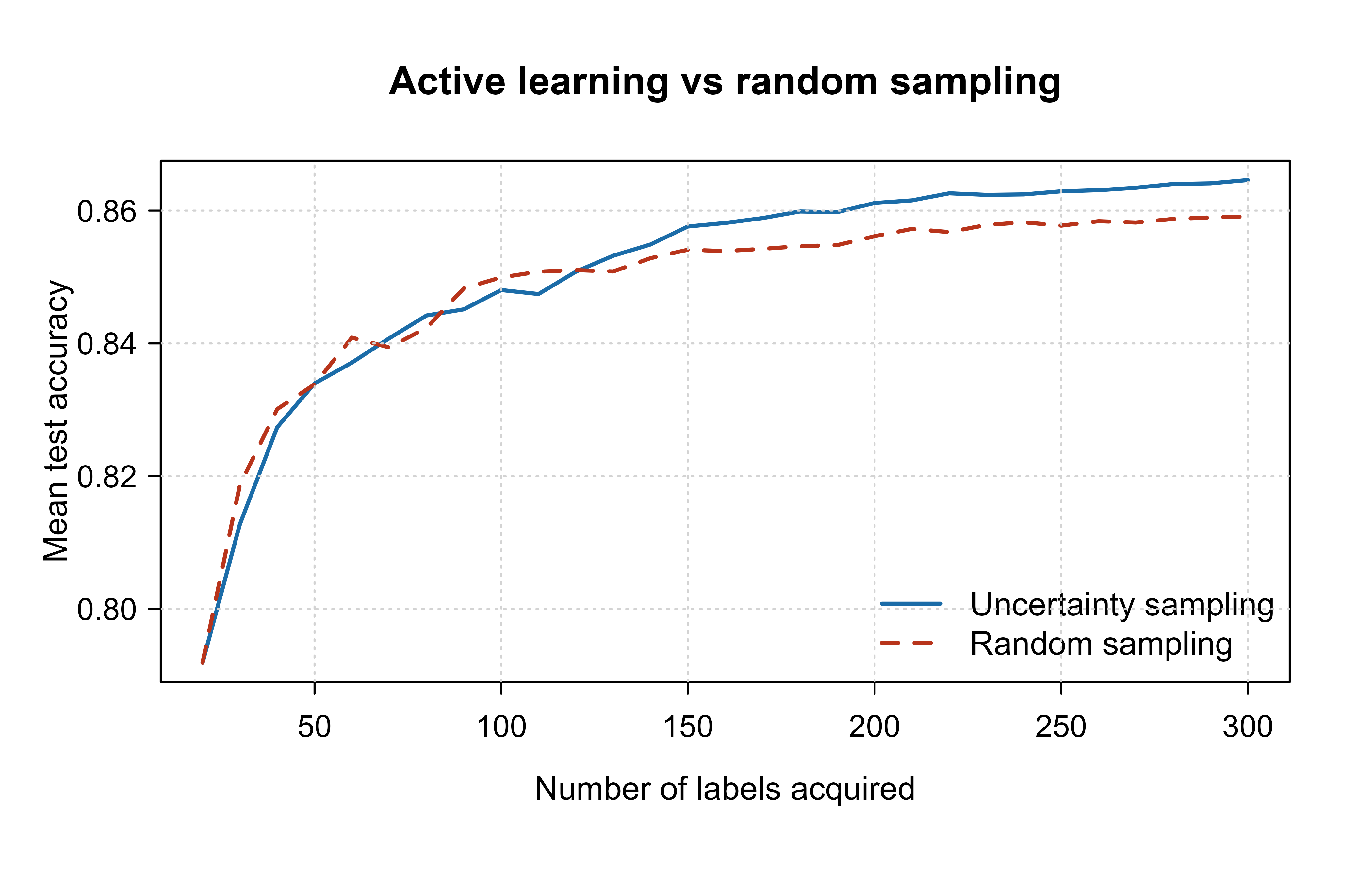
Show code
# Labels each strategy needs to first reach a target accuracy.
labels_to_reach <- function(df, target) {
  hit <- df[df$accuracy >= target, ]
  if (nrow(hit) == 0) return(NA_integer_)
  min(hit$n_labels)
}
target <- 0.86
u_need <- labels_to_reach(ul, target)
r_need <- labels_to_reach(rl, target)
data.frame(
  target_accuracy = target,
  uncertainty_labels = u_need,
  random_labels = r_need
)
#>   target_accuracy uncertainty_labels random_labels
#> 1            0.86                200            NA
The last table reports how many labels each policy needs to first cross a target accuracy. When uncertainty sampling crosses it earlier, the difference is the label budget you save by querying smartly instead of uniformly. (Exact numbers depend on the seed and simulation, so read the gap, not the absolute counts.)
50.7 A note on probabilities and committees
The demo uses raw glm probabilities for the score. Two refinements carry over to real work.
First, uncertainty sampling trusts the model’s probabilities, so calibration matters. A model is calibrated when its stated probabilities match reality: among inputs it labels “70% class 1,” about 70% truly are. If \(\hat{p}\) is overconfident, the “closest to 0.5” set may not be the genuinely ambiguous set. Calibrating probabilities (Platt scaling, isotonic regression; see Chapter 86) before scoring helps.
Warning
A model can be confidently wrong. An overconfident model pushes most predictions toward 0 or 1, so very few points look uncertain, and the ones that do may not be the truly hard cases. Calibrate before you trust an uncertainty score.
The following check confirms the closed form Equation 50.3 for expected gradient length under binary logistic loss, that \(a_{\mathrm{EGL}}(x) = 2\hat p(1-\hat p)\|x\|\). We compute the gradient-norm expectation by brute force (averaging \(\|(\hat p - y)x\|\) over \(y\) with the model’s own weights) and compare to the formula.
Show code
set.seed(7)
beta <- c(0.4, -1.1, 0.7)          # includes intercept
x    <- c(1, 0.8, -0.5)            # one candidate (first entry is intercept term)
phat <- as.numeric(1 / (1 + exp(-sum(beta * x))))

# brute-force expected gradient length: E_y || (phat - y) x ||
egl_brute <- (1 - phat) * sqrt(sum(((phat - 0) * x)^2)) +
             phat       * sqrt(sum(((phat - 1) * x)^2))

# closed form 2 p (1-p) ||x||
egl_form  <- 2 * phat * (1 - phat) * sqrt(sum(x^2))

c(brute = egl_brute, formula = egl_form,
  max_abs_diff = abs(egl_brute - egl_form))
#>        brute      formula max_abs_diff
#>    0.5813769    0.5813769    0.0000000
The two agree to machine precision, and the shared factor \(2\hat p(1-\hat p)\) shows EGL is uncertainty sampling scaled by \(\|x\|\), the scaling that drives its sensitivity to outliers.
Second, query-by-committee needs only a set of differing models. A cheap committee is a handful of bootstrap refits of the same glm (the same resampling idea behind bagging, Chapter 10): resample \(\mathcal{L}\) with replacement, fit each, and score pool points by the variance of their predicted probabilities across committee members. High variance flags disagreement and is a drop-in replacement for the abs(p - 0.5) score above.
50.8 Practical guidance
The strategies above sound like a free win, and often they are. But the same focus that makes active learning efficient also gives it sharp edges. This section collects the conditions under which it pays off and the failure modes to watch for.
Active learning tends to help when these three conditions hold together:
- Labels are expensive and unlabeled data is abundant.
- The model class is a reasonable fit for the data, so its uncertainty estimates mean something.
- You can retrain cheaply enough to run several query rounds.
Just as often, though, the strategy backfires in predictable ways. Watch for the following:
- Cold start. Early on, the seed model is bad and its uncertainty is noise. Begin with a random or diversity-based seed batch before switching to uncertainty.
- Sampling bias. Uncertainty sampling deliberately builds a non-random, boundary-heavy labeled set. That set is great for fitting the boundary but is not a representative sample, so do not use it to estimate class priors or population statistics, and keep a separate random test set for honest evaluation.
- Outliers and label noise. Uncertainty scores spike on garbage inputs and mislabeled points, so the strategy can waste budget querying noise. Filter obvious outliers first (see Chapter 87), and consider density-weighted scores \(a(x) \cdot \mathrm{density}(x)^\beta\) that down-weight isolated points.
- Redundant batches. Top-\(k\) by uncertainty often selects near-duplicate points clustered on one stretch of the boundary. Batch-mode methods add a diversity term (cluster the candidate set, or use determinantal point processes) so a batch covers different regions.
- Model and oracle drift. If the labeling guidelines or the data distribution shift mid-collection, earlier queries may no longer reflect what you need.
- Reproducibility. Because the labeled set depends on the model that selected it, results are tied to the strategy and seeds. Log which strategy chose each label.
Key idea
The actively chosen labels are deliberately biased toward the decision boundary, so they are excellent training data but a terrible random sample. Never estimate population quantities (class frequencies, base rates) from them, and always evaluate on a separate, randomly drawn test set.
50.8.1 Batch-mode active learning, made precise
The redundancy failure above has a formal cause. Top-\(k\) selection treats the batch score as additive, \(\sum_{x \in S} a(x)\), which is maximized by the \(k\) individually highest-scoring points, with no penalty for picking near-duplicates. Because uncertainty is locally smooth, the top-\(k\) set clusters on one stretch of boundary and the \(k\) labels carry little more information than one. Real batch methods replace the additive score by a submodular set objective \(F(S)\) that exhibits diminishing returns, \(F(S \cup \{x\}) - F(S) \ge F(T \cup \{x\}) - F(T)\) for \(S \subseteq T\), so a point already represented in \(S\) contributes little. Two concrete choices:
- A facility-location or core-set objective \(F(S) = -\sum_{x' \in \mathcal{U}} \min_{x \in S}\,\mathrm{dist}(x', x)\) rewards a batch that covers the pool (Sener and Savarese, 2018). Greedy maximization of a monotone submodular \(F\) is guaranteed within a factor \(1 - 1/e \approx 0.63\) of the optimum, which is why greedy batch selection is both cheap and near-optimal.
- A determinantal point process scores a batch by \(\det(K_S)\), the Gram determinant of a kernel \(K\) restricted to \(S\); this is the squared volume spanned by the chosen points, so it is large only when they are both high-quality (large diagonal, encoding \(a(x)\)) and mutually dissimilar (small off-diagonal correlations). It trades off informativeness and diversity in a single determinant.
A pragmatic middle ground, used in BADGE (Ash et al., 2020), embeds each candidate by its loss gradient \(g_x = \nabla_\theta \ell((x, \hat y); \hat\theta)\) at its predicted label (the EGL vector of Section 50.4.3.1), then runs \(k\)-means++ seeding on \(\{g_x\}\). The gradient magnitude encodes uncertainty and the angular spread encodes diversity, so one geometric step buys both at once.
Putting the cautions together, here is a sensible default recipe: seed with a small random (or clustered) batch, use margin or entropy sampling with calibrated probabilities, query in modest batches with a light diversity penalty, and always evaluate on a fixed random held-out set rather than on the actively chosen data.
50.9 Further reading
- Settles, B. (2009, revised 2012). Active Learning Literature Survey and Active Learning (Synthesis Lectures on AI and ML). The standard reference for query strategies and settings.
- Lewis, D. D., and Gale, W. A. (1994). A sequential algorithm for training text classifiers. The origin of uncertainty sampling.
- Seung, H. S., Opper, M., and Sompolinsky, H. (1992). Query by committee.
- Cohn, D. A., Ghahramani, Z., and Jordan, M. I. (1996). Active learning with statistical models.
- Sener, O., and Savarese, S. (2018). Active learning for convolutional neural networks: a core-set approach. A diversity-driven, batch-mode view that scales to deep models.
- Gal, Y., Islam, R., and Ghahramani, Z. (2017). Deep Bayesian active learning with image data (BALD with MC dropout).
An oracle is whatever can supply a true label on demand: a human annotator, a panel of raters, or a physical measurement. The word just means “the thing we pay to get a label,” with no assumption that it is infallible.↩︎
Setting \(\tau\) is the hard part: too low and you exhaust the budget on the first day’s traffic, too high and you finish the month with labels unspent. A common fix is to track recent spend and nudge \(\tau\) up or down to stay on pace.↩︎
The Kullback-Leibler divergence \(\mathrm{KL}(p \,\|\, q) = \sum_y p(y)\log\frac{p(y)}{q(y)}\) measures how far one probability distribution sits from another. Here it measures how far each committee member’s prediction sits from the group consensus, so a large value flags a member that strongly disagrees.↩︎