Advanced Data Analysis

Nguyen, Mike

85 Conformal Prediction and Uncertainty Quantification

A trained regression model hands back a single number for each new input. Ask a gradient-boosted model how long a machine will run before failing and it answers “412 hours,” with no hint of whether the true value is almost certainly between 400 and 420 or could plausibly be anywhere from 100 to 800. For many decisions that silence is unacceptable. A doctor deciding whether to operate, a lender deciding how much to advance, an engineer deciding when to schedule maintenance: each needs to know not just the best guess but a range that is honest about what the model does not know. Uncertainty quantification is the business of producing that range, and conformal prediction is a remarkably general way to do it.

The usual approaches to prediction intervals come with strings attached. Ordinary least squares gives a clean interval formula, but it rests on the assumption that the errors are normal with constant variance, and it is built for linear models. Bayesian methods give credible intervals, but their honesty depends on the prior and the likelihood being right. Bootstrap intervals relax some of this but lean on asymptotics and can be slow. What we would really like is a procedure that wraps around any model we already trust for point prediction (a random forest (Chapter 13), a neural network (Chapter 15), a boosted tree (Chapter 11), even a black box we did not build) and returns an interval that is guaranteed to contain the truth a stated fraction of the time, without assuming anything about the shape of the error distribution. That is exactly what conformal prediction delivers.

Key idea

Conformal prediction converts any point predictor into a set-valued predictor with a finite-sample, distribution-free coverage guarantee. Choose a miscoverage level $\alpha$ (say $0.1$). The method returns prediction sets that contain the true outcome with probability at least $1 - \alpha$ (here $90\%$), and this holds for any data distribution, any model, and any sample size, requiring only that the data are exchangeable.

The phrase “distribution-free” is the part that surprises people. We are not assuming normal errors, not assuming the model is correctly specified, not even assuming the model is any good. A terrible model still gets a valid coverage guarantee from conformal prediction; the price for a bad model is paid in width, not in coverage. A poor model produces honest but wide intervals, while a sharp model produces honest and narrow ones. Coverage is protected unconditionally; usefulness is what improves as the model improves.

In this chapter you will learn the mechanics of split (inductive) conformal prediction, the one-line proof of why it works, how the choice of nonconformity score shapes the resulting sets, and how conformalized quantile regression adapts interval width to local difficulty. We then build the whole thing from scratch in base R, run a simulation, and check empirically that the realized coverage lands where the theory says it should. The foundational references are Vovk, Gammerman, and Shafer (2005) for the original framework and Lei et al. (2018) for the split-conformal regression treatment we follow most closely; Angelopoulos and Bates (2023) is an excellent modern tutorial.

85.1 The setup and the exchangeability assumption

We observe training data $(X_1, Y_1), \dots, (X_n, Y_n)$ and want to predict the outcome $Y_{n+1}$ for a new input $X_{n+1}$. Here $X_i$ is a vector of features and $Y_i \in \mathbb{R}$ is a continuous response. Rather than return a single $\hat{Y}_{n+1}$, we will return a set $C(X_{n+1}) \subseteq \mathbb{R}$, ideally an interval, that we promise contains $Y_{n+1}$ with high probability.

The only assumption is exchangeability: the joint distribution of the data is unchanged under any permutation of the indices. Formally, for any permutation $\pi$,

\[ (X_1, Y_1), \dots, (X_{n+1}, Y_{n+1}) \;\overset{d}{=}\; (X_{\pi(1)}, Y_{\pi(1)}), \dots, (X_{\pi(n+1)}, Y_{\pi(n+1)}). \]

Independent and identically distributed (i.i.d.) data are exchangeable, so the assumption is weaker than i.i.d. and covers the cases most practitioners care about. The point of stating it carefully is to know when conformal prediction can fail: if the future is drawn from a different distribution than the past (distribution shift, time trends, feedback loops), exchangeability breaks and the guarantee no longer holds.

Warning

Exchangeability is the load-bearing assumption. Time series with trends, data that drift after deployment, or test points systematically different from calibration points all violate it, and coverage can degrade quietly. Conformal prediction is distribution-free, not assumption-free.

85.2 Nonconformity scores

The engine of conformal prediction is a nonconformity score, a number $s(x, y)$ that measures how unusual the pair $(x, y)$ looks relative to what the model learned. Large scores mean “this outcome does not conform to the pattern”; small scores mean “this fits right in.” The method is agnostic about how the score is defined, which is the source of its flexibility, but the natural choice for regression is the absolute residual:

\[ s(x, y) = |y - \hat{\mu}(x)|, \]

where $\hat{\mu}$ is the fitted model. A point whose true outcome lands far from the prediction has a large residual and is nonconforming; a point near the prediction conforms. Different scores produce different prediction sets with different shapes, and choosing the score well is the main lever a practitioner has over the quality of the intervals. We will see two scores in this chapter: the plain absolute residual above, which yields constant-width intervals, and a locally adaptive score from conformalized quantile regression, which yields variable-width intervals.

85.3 Split (inductive) conformal prediction

The original “full” conformal method is elegant but expensive: it refits the model for every candidate value of $y$. Split conformal prediction, introduced in this regression form by Lei et al. (2018), trades a little statistical efficiency for an enormous gain in speed by splitting the data once. It is the version used in practice almost everywhere, and it is what we implement.

The recipe has four steps.

Split the data into a proper training set of size $n_t$ and a calibration set of size $n_c$, disjoint from each other.
Fit the model $\hat{\mu}$ on the training set only. The calibration set is never seen during fitting.
Compute the nonconformity score for every calibration point: $s_i = |Y_i - \hat{\mu}(X_i)|$ for each $i$ in the calibration set.
Find the conformal quantile $\hat{q}$, a particular order statistic of the calibration scores (defined precisely below), and form the interval \[ C(X_{n+1}) = \big[\, \hat{\mu}(X_{n+1}) - \hat{q}, \;\; \hat{\mu}(X_{n+1}) + \hat{q} \,\big]. \]

The crucial detail is the finite-sample correction in step 4. We do not take the ordinary $(1-\alpha)$ empirical quantile of the calibration scores. Instead we take the

\[ \frac{\lceil (n_c + 1)(1 - \alpha) \rceil}{n_c} \]

empirical quantile, equivalently the $\lceil (n_c + 1)(1 - \alpha) \rceil$-th smallest of the $n_c$ calibration scores. The “$+1$” accounts for the test point being one more exchangeable draw, and it is what turns an approximate guarantee into an exact one. Skipping it costs a little coverage when $n_c$ is small.

Intuition

The calibration scores are a sample of “how far off the model typically is.” If you want to cover $90\%$ of future points, find the residual size that $90\%$ of calibration residuals fall under, then pad the prediction by that amount in both directions. The $(n_c+1)$ tweak is the bookkeeping that makes “about $90\%$” into “provably at least $90\%$.”

85.3.1 The coverage theorem

Here is the guarantee, stated for the absolute-residual score and the interval above.

Theorem (split-conformal coverage, Lei et al. (2018))

If $(X_1, Y_1), \dots, (X_{n+1}, Y_{n+1})$ are exchangeable and $\hat{q}$ is the $\lceil (n_c+1)(1-\alpha)\rceil$-th smallest calibration score, then \[ \Pr\!\big(Y_{n+1} \in C(X_{n+1})\big) \;\ge\; 1 - \alpha. \] If in addition the scores have no ties (a continuous distribution), the probability is also bounded above by $1 - \alpha + 1/(n_c + 1)$, so coverage is tight, not merely conservative.

The proof is short enough to give in full, and seeing it removes the mystery.

The test point belongs to the interval exactly when its own nonconformity score is no larger than $\hat{q}$:

\[ Y_{n+1} \in C(X_{n+1}) \iff |Y_{n+1} - \hat{\mu}(X_{n+1})| \le \hat{q} \iff s_{n+1} \le \hat{q}. \]

Now condition on the fitted model $\hat{\mu}$ (trained only on the proper training set). The calibration scores $s_1, \dots, s_{n_c}$ and the test score $s_{n+1}$ are functions of exchangeable data points that $\hat{\mu}$ never touched, so these $n_c + 1$ scores are themselves exchangeable. By symmetry, $s_{n+1}$ is equally likely to occupy any rank among the $n_c + 1$ scores when sorted. Setting $\hat{q}$ to the $k$-th smallest with $k = \lceil (n_c+1)(1-\alpha)\rceil$ means

\[ \Pr(s_{n+1} \le \hat{q}) = \Pr(\text{rank of } s_{n+1} \le k) = \frac{k}{n_c + 1} = \frac{\lceil (n_c+1)(1-\alpha)\rceil}{n_c+1} \ge 1 - \alpha. \]

That is the entire argument. No distributional assumption entered; only exchangeability and a counting argument about ranks. The guarantee holds for every sample size, which is what “finite-sample” means.

Note

The probability in the theorem is marginal: it averages over the randomness in both the calibration draw and the test point. It does not promise $90\%$ coverage for every individual $x$. The distinction between marginal and conditional coverage is important enough that we return to it below.

85.4 Marginal versus conditional coverage

Split conformal prediction guarantees marginal coverage: averaged over all future test points, at least $1-\alpha$ land inside their intervals. What it does not guarantee is conditional coverage, the stronger property that

\[ \Pr\!\big(Y_{n+1} \in C(X_{n+1}) \mid X_{n+1} = x\big) \ge 1 - \alpha \quad \text{for every } x. \]

The difference matters whenever prediction difficulty varies across the feature space. With the constant-width absolute-residual interval, the half-width $\hat{q}$ is the same for every $x$. In regions where the outcome is easy to predict, that fixed width over-covers (the interval is wider than it needs to be); in regions where the outcome is volatile, it under-covers (too narrow). The marginal average can still be exactly $1-\alpha$ while some subgroups sit well above and others well below.

Intuition

A constant-width interval is like a single jacket size handed to a whole population. On average the fit is acceptable, but it is baggy on small people and tight on large ones. Conditional coverage asks the interval to fit everyone reasonably, which means letting the width change with $x$.

Exact distribution-free conditional coverage is impossible in finite samples without further assumptions (a result of Vovk (2012) and Lei and Wasserman (2014)). But we can get much closer in practice by choosing a nonconformity score that already knows local difficulty. That is the motivation for conformalized quantile regression.

85.5 Conformalized quantile regression

Conformalized quantile regression (CQR), due to Romano, Patterson, and Candes (2019), combines the local adaptivity of quantile regression (Chapter 21) with the coverage guarantee of conformal prediction. The idea is to start from a model that already produces a variable-width band and then conformalize it so the coverage is exact.

Fit two conditional quantile estimates on the training set: a lower quantile $\hat{q}_{\alpha/2}(x)$ and an upper quantile $\hat{q}_{1-\alpha/2}(x)$ (for $\alpha = 0.1$, the $5$th and $95$th percentiles). These already form a candidate interval $[\hat{q}_{\alpha/2}(x), \hat{q}_{1-\alpha/2}(x)]$ whose width adapts to $x$, but quantile regression offers no finite-sample coverage promise, so we calibrate it. The CQR nonconformity score measures how far a calibration point falls outside the candidate band, signed so that points inside the band get negative scores:

\[ s_i = \max\!\big\{\, \hat{q}_{\alpha/2}(X_i) - Y_i, \;\; Y_i - \hat{q}_{1-\alpha/2}(X_i) \,\big\}. \]

If $Y_i$ sits inside the band both terms are negative and the score is negative; if it pokes out the bottom the first term is the positive overshoot; if it pokes out the top the second term is. We then take the conformal quantile $\hat{q}$ of these scores exactly as before (the $\lceil (n_c+1)(1-\alpha)\rceil$-th smallest) and form

\[ C(x) = \big[\, \hat{q}_{\alpha/2}(x) - \hat{q}, \;\; \hat{q}_{1-\alpha/2}(x) + \hat{q} \,\big]. \]

The same exchangeability proof gives the same $1-\alpha$ marginal guarantee, because nothing in that argument depended on the score being an absolute residual. The reward is that the interval inherits the variable width of the quantile band: it widens where the data are volatile and narrows where they are calm, so conditional coverage is much more even than for the constant-width method, while marginal coverage stays exact.

Key idea

CQR keeps the exact marginal guarantee of split conformal prediction and adds local adaptivity by conformalizing a quantile-regression band instead of a mean prediction. You give up nothing on coverage and gain intervals that breathe with the difficulty of the input.

85.6 A simulation in base R

We now build split conformal prediction from scratch and verify the coverage guarantee empirically. The data are deliberately heteroskedastic (the noise grows with $x$) so that the difference between constant-width and adaptive intervals is visible. We fit an ordinary linear model as the point predictor, conformalize its residuals, and form prediction intervals on a held-out test set.

Show code

set.seed(1301)

# data-generating process: nonlinear mean, growing (heteroskedastic) noise
gen_data <- function(n) {
  x <- runif(n, 0, 10)
  mu <- 2 + 1.5 * sin(x) + 0.5 * x           # true conditional mean
  sigma <- 0.3 + 0.25 * x                     # noise grows with x
  y <- mu + rnorm(n, 0, sigma)
  data.frame(x = x, y = y)
}

n_total <- 3000
dat <- gen_data(n_total)

# three-way split: proper training, calibration, test
idx <- sample(rep(c("train", "calib", "test"), length.out = n_total))
train <- dat[idx == "train", ]
calib <- dat[idx == "calib", ]
test  <- dat[idx == "test",  ]

alpha <- 0.1   # target 90% coverage

With the data split, we fit the point predictor on the training set only, score the calibration set, and read off the conformal quantile with the finite-sample correction.

Show code

# step 2: fit the point predictor on training data only
fit <- lm(y ~ poly(x, 3), data = train)

# step 3: absolute-residual nonconformity scores on the calibration set
mu_hat_calib <- predict(fit, newdata = calib)
scores <- abs(calib$y - mu_hat_calib)

# step 4: conformal quantile with the (n_c + 1) finite-sample correction
n_c <- nrow(calib)
k <- ceiling((n_c + 1) * (1 - alpha))
q_hat <- sort(scores)[k]
q_hat
#>     1265 
#> 3.161541

The number q_hat is the half-width of every prediction interval. We now form intervals on the test set and measure how often the true outcome falls inside.

Show code

# split-conformal intervals on the test set
mu_hat_test <- predict(fit, newdata = test)
lower <- mu_hat_test - q_hat
upper <- mu_hat_test + q_hat

covered <- (test$y >= lower) & (test$y <= upper)
emp_coverage <- mean(covered)
avg_width <- mean(upper - lower)

c(target = 1 - alpha, empirical = emp_coverage, avg_width = avg_width)
#>    target empirical avg_width 
#>  0.900000  0.913000  6.323083

The empirical coverage lands at roughly the target $0.90$, as the theorem promises. A single split is itself random, so the realized coverage fluctuates around $1-\alpha$ from one split to the next. To see that the guarantee holds on average rather than by luck, we repeat the entire split-fit-calibrate-test cycle many times and look at the distribution of realized coverage.

Show code

run_once <- function() {
  d <- gen_data(n_total)
  ix <- sample(rep(c("train", "calib", "test"), length.out = n_total))
  tr <- d[ix == "train", ]; ca <- d[ix == "calib", ]; te <- d[ix == "test", ]
  f <- lm(y ~ poly(x, 3), data = tr)
  s <- abs(ca$y - predict(f, newdata = ca))
  nc <- nrow(ca)
  qh <- sort(s)[ceiling((nc + 1) * (1 - alpha))]
  mh <- predict(f, newdata = te)
  mean(te$y >= mh - qh & te$y <= mh + qh)
}

set.seed(42)
cov_reps <- replicate(200, run_once())
mean(cov_reps)
#> [1] 0.89906

The mean of the realized coverages sits essentially on $0.90$, which is the marginal guarantee made visible.

85.6.1 Comparing the methods

To make the marginal-versus-conditional distinction concrete, we also fit conformalized quantile regression on the same data and compare it to the constant-width method. We use linear quantile regression from the quantreg package for the lower and upper quantile estimates.

Show code

library(quantreg)

# fit lower and upper conditional quantiles on the training set
lo_fit <- rq(y ~ poly(x, 3), data = train, tau = alpha / 2)
hi_fit <- rq(y ~ poly(x, 3), data = train, tau = 1 - alpha / 2)

# CQR nonconformity scores on the calibration set
lo_calib <- predict(lo_fit, newdata = calib)
hi_calib <- predict(hi_fit, newdata = calib)
cqr_scores <- pmax(lo_calib - calib$y, calib$y - hi_calib)

k_cqr <- ceiling((n_c + 1) * (1 - alpha))
q_cqr <- sort(cqr_scores)[k_cqr]

# conformalized intervals on the test set
lo_test <- predict(lo_fit, newdata = test) - q_cqr
hi_test <- predict(hi_fit, newdata = test) + q_cqr

cqr_covered <- (test$y >= lo_test) & (test$y <= hi_test)
cqr_coverage <- mean(cqr_covered)
cqr_avg_width <- mean(hi_test - lo_test)

Both methods hit the marginal target, so the interesting comparison is conditional coverage and width across the range of $x$. We bin the test points by $x$ and compute coverage within each bin for both methods. Table 85.1 summarizes the overall numbers.

Show code

methods_tab <- data.frame(
  Method = c("Split conformal (abs. residual)", "Conformalized quantile reg."),
  `Target coverage` = c(1 - alpha, 1 - alpha),
  `Empirical coverage` = round(c(emp_coverage, cqr_coverage), 3),
  `Average width` = round(c(avg_width, cqr_avg_width), 3),
  `Interval width` = c("constant", "adapts to x"),
  check.names = FALSE
)
knitr::kable(
  methods_tab,
  caption = "Marginal coverage and average interval width for constant-width split conformal prediction versus conformalized quantile regression on the heteroskedastic test set. Both achieve the target marginal coverage; CQR achieves it with intervals whose width varies across the input."
)

Table 85.1: Marginal coverage and average interval width for constant-width split conformal prediction versus conformalized quantile regression on the heteroskedastic test set. Both achieve the target marginal coverage; CQR achieves it with intervals whose width varies across the input.

Method	Target coverage	Empirical coverage	Average width	Interval width
Split conformal (abs. residual)	0.9	0.913	6.323	constant
Conformalized quantile reg.	0.9	0.908	5.956	adapts to x

Table 85.1 shows the key trade-off: both procedures cover at the marginal $90\%$ level, but they get there differently. The constant-width method pays for the noisy region by being wide everywhere, while CQR concentrates its width where the data demand it.

Table 85.2 breaks coverage down by region of $x$, exposing the gap between marginal and conditional coverage for the constant-width method.

Show code

bins <- cut(test$x, breaks = c(0, 2.5, 5, 7.5, 10), include.lowest = TRUE)
cond_tab <- data.frame(
  `x range` = levels(bins),
  `Split-conformal coverage` = round(tapply(covered, bins, mean), 3),
  `Split-conformal width`    = round(tapply(upper - lower, bins, mean), 3),
  `CQR coverage`             = round(tapply(cqr_covered, bins, mean), 3),
  `CQR width`                = round(tapply(hi_test - lo_test, bins, mean), 3),
  check.names = FALSE,
  row.names = NULL
)
knitr::kable(
  cond_tab,
  caption = "Coverage and average interval width by region of the predictor x. The constant-width split-conformal method over-covers where the data are calm (small x) and drifts toward under-coverage where they are noisy (large x), while conformalized quantile regression keeps coverage steadier across regions by widening its intervals with x."
)

Table 85.2: Coverage and average interval width by region of the predictor x. The constant-width split-conformal method over-covers where the data are calm (small x) and drifts toward under-coverage where they are noisy (large x), while conformalized quantile regression keeps coverage steadier across regions by widening its intervals with x.

x range	Split-conformal coverage	Split-conformal width	CQR coverage	CQR width
[0,2.5]	1.000	6.323	0.950	3.635
(2.5,5]	0.955	6.323	0.853	4.420
(5,7.5]	0.876	6.323	0.908	6.788
(7.5,10]	0.819	6.323	0.926	9.074

Table 85.2 is the heart of the comparison. Reading across the rows, the constant-width method’s per-region coverage swings above and below the $0.90$ target as $x$ moves, even though the overall average is on target, because a single half-width cannot fit both the calm low-$x$ region and the volatile high-$x$ region. CQR’s width column climbs with $x$, and its per-region coverage stays closer to the target throughout. This is the marginal-versus-conditional story in numbers.

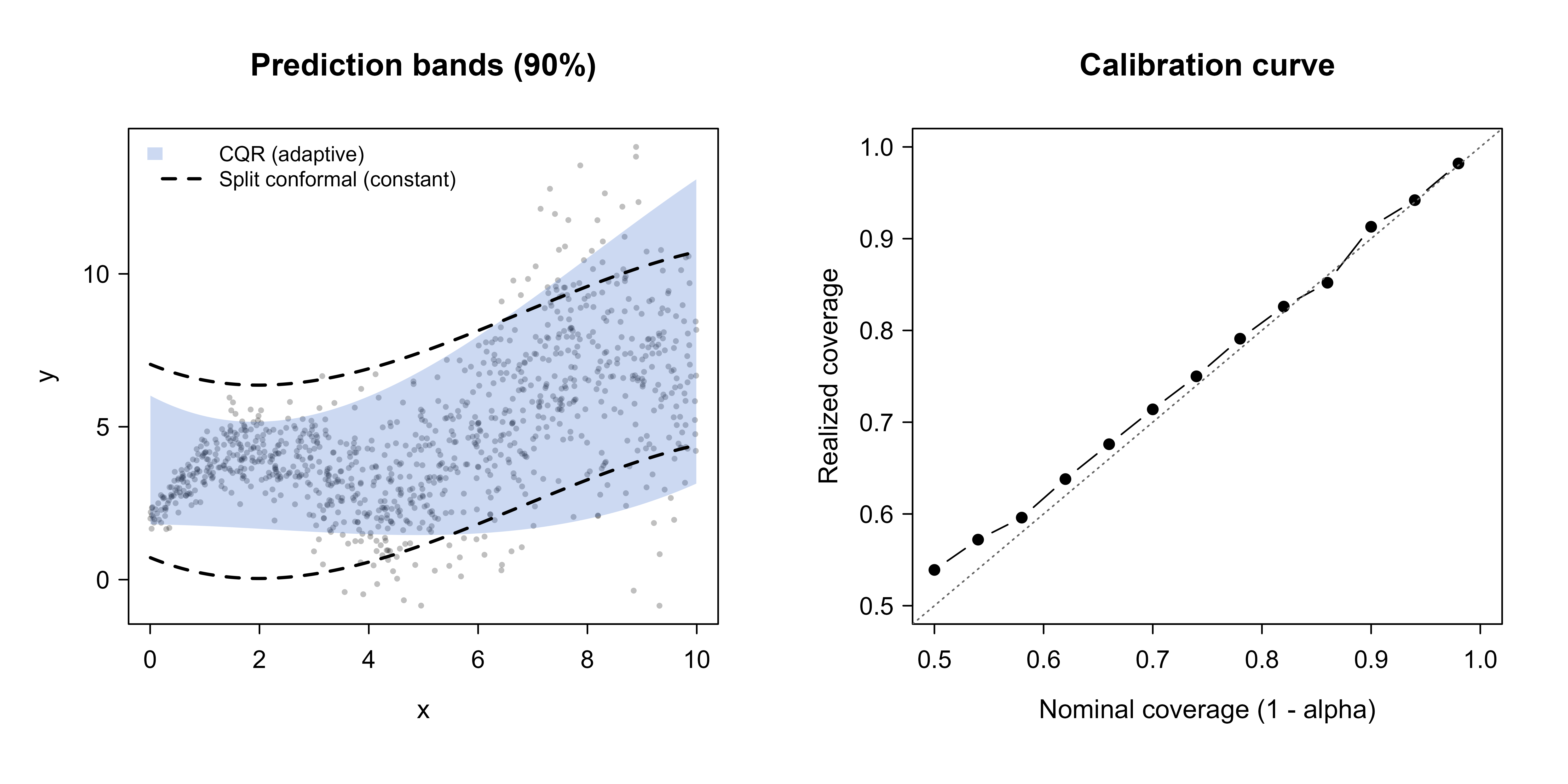
85.6.2 A coverage and calibration figure

Two pictures make the behavior concrete. The first shows the prediction bands over the data; the second checks calibration by sweeping the target coverage level and plotting realized against nominal coverage. Both panels are drawn in a single chunk with par(mfrow=...) so they form one figure.

Show code

ord <- order(test$x)
xs  <- test$x[ord]

par(mfrow = c(1, 2))

# left panel: the two prediction bands over the data
plot(test$x, test$y, pch = 16, col = rgb(0, 0, 0, 0.25), cex = 0.5,
     xlab = "x", ylab = "y", main = "Prediction bands (90%)")
polygon(c(xs, rev(xs)), c(lo_test[ord], rev(hi_test[ord])),
        col = rgb(0.2, 0.4, 0.8, 0.25), border = NA)
lines(xs, (mu_hat_test - q_hat)[ord], lty = 2, lwd = 2)
lines(xs, (mu_hat_test + q_hat)[ord], lty = 2, lwd = 2)
legend("topleft", c("CQR (adaptive)", "Split conformal (constant)"),
       fill = c(rgb(0.2, 0.4, 0.8, 0.25), NA),
       border = c(NA, NA), lty = c(NA, 2), lwd = c(NA, 2),
       bty = "n", cex = 0.8)

# right panel: calibration curve, realized vs nominal coverage
nominal <- seq(0.5, 0.98, by = 0.04)
realized <- sapply(nominal, function(lev) {
  kk <- ceiling((n_c + 1) * lev)
  kk <- min(kk, n_c)
  qq <- sort(scores)[kk]
  mean(abs(test$y - mu_hat_test) <= qq)
})
plot(nominal, realized, type = "b", pch = 16,
     xlim = c(0.5, 1), ylim = c(0.5, 1),
     xlab = "Nominal coverage (1 - alpha)", ylab = "Realized coverage",
     main = "Calibration curve")
abline(0, 1, lty = 3, col = "grey40")

Figure 85.1: Left: split-conformal (constant width, dashed) and conformalized quantile regression (adaptive, shaded) 90 percent prediction bands over the heteroskedastic test data; the adaptive band widens with x while the constant band does not. Right: a calibration curve sweeping the nominal level 1 minus alpha against realized coverage for the split-conformal method, lying close to the 45-degree line, which is the empirical signature of a valid distribution-free interval.

Figure 85.1 shows both effects at once. In the left panel the constant-width dashed band is too wide at small $x$ and too narrow at large $x$, while the shaded CQR band tracks the growing noise. In the right panel the realized coverage follows the $45$-degree line across the whole range of nominal levels, which is the visual confirmation that the conformal intervals are valid at every target coverage, not just at $\alpha = 0.1$.

85.7 Practical guidance and pitfalls

Conformal prediction is simple to get right and easy to misuse in a few specific ways. A handful of points cover most of what goes wrong in practice.

The calibration set must be genuinely held out. The proof breaks the moment the calibration data influence the fitted model, so any data used in training, hyperparameter tuning, or feature selection cannot also serve as calibration. Reusing points silently inflates coverage claims.

Size the calibration set sensibly. Because $\hat{q}$ is an order statistic, very small calibration sets make it jumpy from split to split, and with $n_c$ too small the achievable coverage levels become coarse (you cannot ask for $99\%$ coverage with only $20$ calibration points, since $\lceil 21 \times 0.99 \rceil = 21 > 20$). A few hundred to a few thousand calibration points give stable, fine-grained quantiles. A rough rule is $n_c \ge 1/\alpha$ at the very least, and comfortably more in practice.

Do not skip the $+1$ correction. Using the plain empirical quantile instead of the $\lceil (n_c+1)(1-\alpha)\rceil$ order statistic loses a sliver of coverage that matters when $n_c$ is small. The correction is one line of code and makes the guarantee exact.

Match the score to what you care about. The absolute-residual score gives constant-width intervals that are fine when the noise is homoskedastic, but for heteroskedastic data a locally adaptive score such as CQR (or normalizing the residual by an estimate of local spread) gives far more even conditional coverage at the same marginal level. Reach for an adaptive score whenever prediction difficulty varies across the feature space.

Warning

Watch for distribution shift. The single biggest failure mode in deployment is that test data stop being exchangeable with calibration data: covariates drift, the target relationship changes, or model outputs feed back into the system. When that happens, coverage degrades without any error message. For sequential or shifting data, look at extensions such as adaptive conformal inference (Gibbs and Candes (2021)) and weighted conformal prediction (Tibshirani et al. (2019)), which relax exchangeability in controlled ways.

When to use this

Use conformal prediction whenever you need honest, distribution-free uncertainty bands around an existing point predictor and your data are (approximately) exchangeable. It shines as a thin wrapper around black-box models where you cannot or do not want to assume an error distribution. Prefer CQR or another adaptive score when conditional coverage matters; the plain residual score is enough when the noise is roughly uniform across inputs.

A last point on interpretation. Conformal coverage is marginal by default, so a reported $90\%$ interval means $90\%$ of such intervals contain the truth on average, not that any particular interval has a $90\%$ chance once you condition on its specific $x$. Communicating that distinction to stakeholders prevents the common mistake of reading a single interval as a conditional guarantee.

85.8 Further reading

The framework originates with Vovk, Gammerman, and Shafer (2005), Algorithmic Learning in a Random World, which develops full conformal prediction in detail. Lei, G’Sell, Rinaldo, Tibshirani, and Wasserman (2018) give the split-conformal regression treatment and the coverage theorem followed here. Romano, Patterson, and Cand’es (2019) introduce conformalized quantile regression for locally adaptive intervals. For the impossibility of distribution-free conditional coverage, see Vovk (2012) and Lei and Wasserman (2014). Tibshirani, Barber, Cand’es, and Ramdas (2019) extend the method to covariate shift through weighting, and Gibbs and Cand’es (2021) develop adaptive conformal inference for online and shifting data, connecting to the methods of the online and streaming learning chapter (Chapter 55). Angelopoulos and Bates (2023), Conformal Prediction: A Gentle Introduction, is the most accessible modern entry point and surveys classification, time series, and risk-control extensions.

# Conformal Prediction and Uncertainty Quantification {#sec-conformal-prediction} ```{r} #| include: false source("_common.R") ``` A trained regression model hands back a single number for each new input. Ask a gradient-boosted model how long a machine will run before failing and it answers "412 hours," with no hint of whether the true value is almost certainly between 400 and 420 or could plausibly be anywhere from 100 to 800. For many decisions that silence is unacceptable. A doctor deciding whether to operate, a lender deciding how much to advance, an engineer deciding when to schedule maintenance: each needs to know not just the best guess but a range that is honest about what the model does not know. Uncertainty quantification is the business of producing that range, and conformal prediction is a remarkably general way to do it. The usual approaches to prediction intervals come with strings attached. Ordinary least squares gives a clean interval formula, but it rests on the assumption that the errors are normal with constant variance, and it is built for linear models. Bayesian methods give credible intervals, but their honesty depends on the prior and the likelihood being right. Bootstrap intervals relax some of this but lean on asymptotics and can be slow. What we would really like is a procedure that wraps around *any* model we already trust for point prediction (a random forest (@sec-random-forest), a neural network (@sec-neural-networks), a boosted tree (@sec-boosting), even a black box we did not build) and returns an interval that is guaranteed to contain the truth a stated fraction of the time, without assuming anything about the shape of the error distribution. That is exactly what conformal prediction delivers. ::: {.callout-important title="Key idea"} Conformal prediction converts any point predictor into a set-valued predictor with a finite-sample, distribution-free coverage guarantee. Choose a miscoverage level $\alpha$ (say $0.1$). The method returns prediction sets that contain the true outcome with probability at least $1 - \alpha$ (here $90\%$), and this holds for any data distribution, any model, and any sample size, requiring only that the data are exchangeable. ::: The phrase "distribution-free" is the part that surprises people. We are not assuming normal errors, not assuming the model is correctly specified, not even assuming the model is any good. A terrible model still gets a valid coverage guarantee from conformal prediction; the price for a bad model is paid in *width*, not in *coverage*. A poor model produces honest but wide intervals, while a sharp model produces honest and narrow ones. Coverage is protected unconditionally; usefulness is what improves as the model improves. In this chapter you will learn the mechanics of split (inductive) conformal prediction, the one-line proof of why it works, how the choice of nonconformity score shapes the resulting sets, and how conformalized quantile regression adapts interval width to local difficulty. We then build the whole thing from scratch in base R, run a simulation, and check empirically that the realized coverage lands where the theory says it should. The foundational references are @Vovk_2005 for the original framework and @Lei_2018 for the split-conformal regression treatment we follow most closely; @Angelopoulos_2023 is an excellent modern tutorial. ## The setup and the exchangeability assumption We observe training data $(X_1, Y_1), \dots, (X_n, Y_n)$ and want to predict the outcome $Y_{n+1}$ for a new input $X_{n+1}$. Here $X_i$ is a vector of features and $Y_i \in \mathbb{R}$ is a continuous response. Rather than return a single $\hat{Y}_{n+1}$, we will return a set $C(X_{n+1}) \subseteq \mathbb{R}$, ideally an interval, that we promise contains $Y_{n+1}$ with high probability. The only assumption is exchangeability: the joint distribution of the data is unchanged under any permutation of the indices. Formally, for any permutation $\pi$, $$ (X_1, Y_1), \dots, (X_{n+1}, Y_{n+1}) \;\overset{d}{=}\; (X_{\pi(1)}, Y_{\pi(1)}), \dots, (X_{\pi(n+1)}, Y_{\pi(n+1)}). $$ Independent and identically distributed (i.i.d.) data are exchangeable, so the assumption is weaker than i.i.d. and covers the cases most practitioners care about. The point of stating it carefully is to know when conformal prediction can fail: if the future is drawn from a different distribution than the past (distribution shift, time trends, feedback loops), exchangeability breaks and the guarantee no longer holds. ::: {.callout-warning} Exchangeability is the load-bearing assumption. Time series with trends, data that drift after deployment, or test points systematically different from calibration points all violate it, and coverage can degrade quietly. Conformal prediction is distribution-free, not assumption-free. ::: ## Nonconformity scores The engine of conformal prediction is a nonconformity score, a number $s(x, y)$ that measures how unusual the pair $(x, y)$ looks relative to what the model learned. Large scores mean "this outcome does not conform to the pattern"; small scores mean "this fits right in." The method is agnostic about how the score is defined, which is the source of its flexibility, but the natural choice for regression is the absolute residual: $$ s(x, y) = |y - \hat{\mu}(x)|, $$ where $\hat{\mu}$ is the fitted model. A point whose true outcome lands far from the prediction has a large residual and is nonconforming; a point near the prediction conforms. Different scores produce different prediction sets with different shapes, and choosing the score well is the main lever a practitioner has over the quality of the intervals. We will see two scores in this chapter: the plain absolute residual above, which yields constant-width intervals, and a locally adaptive score from conformalized quantile regression, which yields variable-width intervals. ## Split (inductive) conformal prediction The original "full" conformal method is elegant but expensive: it refits the model for every candidate value of $y$. Split conformal prediction, introduced in this regression form by @Lei_2018, trades a little statistical efficiency for an enormous gain in speed by splitting the data once. It is the version used in practice almost everywhere, and it is what we implement. The recipe has four steps. 1. Split the data into a proper training set of size $n_t$ and a calibration set of size $n_c$, disjoint from each other. 2. Fit the model $\hat{\mu}$ on the training set only. The calibration set is never seen during fitting. 3. Compute the nonconformity score for every calibration point: $s_i = |Y_i - \hat{\mu}(X_i)|$ for each $i$ in the calibration set. 4. Find the conformal quantile $\hat{q}$, a particular order statistic of the calibration scores (defined precisely below), and form the interval $$ C(X_{n+1}) = \big[\, \hat{\mu}(X_{n+1}) - \hat{q}, \;\; \hat{\mu}(X_{n+1}) + \hat{q} \,\big]. $$ The crucial detail is the finite-sample correction in step 4. We do not take the ordinary $(1-\alpha)$ empirical quantile of the calibration scores. Instead we take the $$ \frac{\lceil (n_c + 1)(1 - \alpha) \rceil}{n_c} $$ empirical quantile, equivalently the $\lceil (n_c + 1)(1 - \alpha) \rceil$-th smallest of the $n_c$ calibration scores. The "$+1$" accounts for the test point being one more exchangeable draw, and it is what turns an approximate guarantee into an exact one. Skipping it costs a little coverage when $n_c$ is small. ::: {.callout-tip title="Intuition"} The calibration scores are a sample of "how far off the model typically is." If you want to cover $90\%$ of future points, find the residual size that $90\%$ of calibration residuals fall under, then pad the prediction by that amount in both directions. The $(n_c+1)$ tweak is the bookkeeping that makes "about $90\%$" into "provably at least $90\%$." ::: ### The coverage theorem Here is the guarantee, stated for the absolute-residual score and the interval above. ::: {.callout-note title="Theorem (split-conformal coverage, @Lei_2018)"} If $(X_1, Y_1), \dots, (X_{n+1}, Y_{n+1})$ are exchangeable and $\hat{q}$ is the $\lceil (n_c+1)(1-\alpha)\rceil$-th smallest calibration score, then $$ \Pr\!\big(Y_{n+1} \in C(X_{n+1})\big) \;\ge\; 1 - \alpha. $$ If in addition the scores have no ties (a continuous distribution), the probability is also bounded above by $1 - \alpha + 1/(n_c + 1)$, so coverage is tight, not merely conservative. ::: The proof is short enough to give in full, and seeing it removes the mystery. The test point belongs to the interval exactly when its own nonconformity score is no larger than $\hat{q}$: $$ Y_{n+1} \in C(X_{n+1}) \iff |Y_{n+1} - \hat{\mu}(X_{n+1})| \le \hat{q} \iff s_{n+1} \le \hat{q}. $$ Now condition on the fitted model $\hat{\mu}$ (trained only on the proper training set). The calibration scores $s_1, \dots, s_{n_c}$ and the test score $s_{n+1}$ are functions of exchangeable data points that $\hat{\mu}$ never touched, so these $n_c + 1$ scores are themselves exchangeable. By symmetry, $s_{n+1}$ is equally likely to occupy any rank among the $n_c + 1$ scores when sorted. Setting $\hat{q}$ to the $k$-th smallest with $k = \lceil (n_c+1)(1-\alpha)\rceil$ means $$ \Pr(s_{n+1} \le \hat{q}) = \Pr(\text{rank of } s_{n+1} \le k) = \frac{k}{n_c + 1} = \frac{\lceil (n_c+1)(1-\alpha)\rceil}{n_c+1} \ge 1 - \alpha. $$ That is the entire argument. No distributional assumption entered; only exchangeability and a counting argument about ranks. The guarantee holds for every sample size, which is what "finite-sample" means. ::: {.callout-note} The probability in the theorem is **marginal**: it averages over the randomness in both the calibration draw and the test point. It does not promise $90\%$ coverage for every individual $x$. The distinction between marginal and conditional coverage is important enough that we return to it below. ::: ## Marginal versus conditional coverage Split conformal prediction guarantees marginal coverage: averaged over all future test points, at least $1-\alpha$ land inside their intervals. What it does not guarantee is conditional coverage, the stronger property that $$ \Pr\!\big(Y_{n+1} \in C(X_{n+1}) \mid X_{n+1} = x\big) \ge 1 - \alpha \quad \text{for every } x. $$ The difference matters whenever prediction difficulty varies across the feature space. With the constant-width absolute-residual interval, the half-width $\hat{q}$ is the same for every $x$. In regions where the outcome is easy to predict, that fixed width over-covers (the interval is wider than it needs to be); in regions where the outcome is volatile, it under-covers (too narrow). The marginal average can still be exactly $1-\alpha$ while some subgroups sit well above and others well below. ::: {.callout-tip title="Intuition"} A constant-width interval is like a single jacket size handed to a whole population. On average the fit is acceptable, but it is baggy on small people and tight on large ones. Conditional coverage asks the interval to fit *everyone* reasonably, which means letting the width change with $x$. ::: Exact distribution-free conditional coverage is impossible in finite samples without further assumptions (a result of @Vovk_2012 and @Lei_2014). But we can get much closer in practice by choosing a nonconformity score that already knows local difficulty. That is the motivation for conformalized quantile regression. ## Conformalized quantile regression Conformalized quantile regression (CQR), due to @Romano_2019, combines the local adaptivity of quantile regression (@sec-quantile-reg) with the coverage guarantee of conformal prediction. The idea is to start from a model that already produces a variable-width band and then conformalize it so the coverage is exact. Fit two conditional quantile estimates on the training set: a lower quantile $\hat{q}_{\alpha/2}(x)$ and an upper quantile $\hat{q}_{1-\alpha/2}(x)$ (for $\alpha = 0.1$, the $5$th and $95$th percentiles). These already form a candidate interval $[\hat{q}_{\alpha/2}(x), \hat{q}_{1-\alpha/2}(x)]$ whose width adapts to $x$, but quantile regression offers no finite-sample coverage promise, so we calibrate it. The CQR nonconformity score measures how far a calibration point falls *outside* the candidate band, signed so that points inside the band get negative scores: $$ s_i = \max\!\big\{\, \hat{q}_{\alpha/2}(X_i) - Y_i, \;\; Y_i - \hat{q}_{1-\alpha/2}(X_i) \,\big\}. $$ If $Y_i$ sits inside the band both terms are negative and the score is negative; if it pokes out the bottom the first term is the positive overshoot; if it pokes out the top the second term is. We then take the conformal quantile $\hat{q}$ of these scores exactly as before (the $\lceil (n_c+1)(1-\alpha)\rceil$-th smallest) and form $$ C(x) = \big[\, \hat{q}_{\alpha/2}(x) - \hat{q}, \;\; \hat{q}_{1-\alpha/2}(x) + \hat{q} \,\big]. $$ The same exchangeability proof gives the same $1-\alpha$ marginal guarantee, because nothing in that argument depended on the score being an absolute residual. The reward is that the interval inherits the variable width of the quantile band: it widens where the data are volatile and narrows where they are calm, so conditional coverage is much more even than for the constant-width method, while marginal coverage stays exact. ::: {.callout-important title="Key idea"} CQR keeps the exact marginal guarantee of split conformal prediction and adds local adaptivity by conformalizing a quantile-regression band instead of a mean prediction. You give up nothing on coverage and gain intervals that breathe with the difficulty of the input. ::: ## A simulation in base R We now build split conformal prediction from scratch and verify the coverage guarantee empirically. The data are deliberately heteroskedastic (the noise grows with $x$) so that the difference between constant-width and adaptive intervals is visible. We fit an ordinary linear model as the point predictor, conformalize its residuals, and form prediction intervals on a held-out test set. ```{r conformal-prediction-setup} set.seed(1301) # data-generating process: nonlinear mean, growing (heteroskedastic) noise gen_data <- function(n) { x <- runif(n, 0, 10) mu <- 2 + 1.5 * sin(x) + 0.5 * x # true conditional mean sigma <- 0.3 + 0.25 * x # noise grows with x y <- mu + rnorm(n, 0, sigma) data.frame(x = x, y = y) } n_total <- 3000 dat <- gen_data(n_total) # three-way split: proper training, calibration, test idx <- sample(rep(c("train", "calib", "test"), length.out = n_total)) train <- dat[idx == "train", ] calib <- dat[idx == "calib", ] test <- dat[idx == "test", ] alpha <- 0.1 # target 90% coverage ``` With the data split, we fit the point predictor on the training set only, score the calibration set, and read off the conformal quantile with the finite-sample correction. ```{r conformal-prediction-split} # step 2: fit the point predictor on training data only fit <- lm(y ~ poly(x, 3), data = train) # step 3: absolute-residual nonconformity scores on the calibration set mu_hat_calib <- predict(fit, newdata = calib) scores <- abs(calib$y - mu_hat_calib) # step 4: conformal quantile with the (n_c + 1) finite-sample correction n_c <- nrow(calib) k <- ceiling((n_c + 1) * (1 - alpha)) q_hat <- sort(scores)[k] q_hat ``` The number `q_hat` is the half-width of every prediction interval. We now form intervals on the test set and measure how often the true outcome falls inside. ```{r conformal-prediction-coverage} # split-conformal intervals on the test set mu_hat_test <- predict(fit, newdata = test) lower <- mu_hat_test - q_hat upper <- mu_hat_test + q_hat covered <- (test$y >= lower) & (test$y <= upper) emp_coverage <- mean(covered) avg_width <- mean(upper - lower) c(target = 1 - alpha, empirical = emp_coverage, avg_width = avg_width) ``` The empirical coverage lands at roughly the target $0.90$, as the theorem promises. A single split is itself random, so the realized coverage fluctuates around $1-\alpha$ from one split to the next. To see that the guarantee holds on average rather than by luck, we repeat the entire split-fit-calibrate-test cycle many times and look at the distribution of realized coverage. ```{r conformal-prediction-repeat} run_once <- function() { d <- gen_data(n_total) ix <- sample(rep(c("train", "calib", "test"), length.out = n_total)) tr <- d[ix == "train", ]; ca <- d[ix == "calib", ]; te <- d[ix == "test", ] f <- lm(y ~ poly(x, 3), data = tr) s <- abs(ca$y - predict(f, newdata = ca)) nc <- nrow(ca) qh <- sort(s)[ceiling((nc + 1) * (1 - alpha))] mh <- predict(f, newdata = te) mean(te$y >= mh - qh & te$y <= mh + qh) } set.seed(42) cov_reps <- replicate(200, run_once()) mean(cov_reps) ``` The mean of the realized coverages sits essentially on $0.90$, which is the marginal guarantee made visible. ### Comparing the methods To make the marginal-versus-conditional distinction concrete, we also fit conformalized quantile regression on the same data and compare it to the constant-width method. We use linear quantile regression from the `quantreg` package for the lower and upper quantile estimates. ```{r conformal-prediction-cqr} library(quantreg) # fit lower and upper conditional quantiles on the training set lo_fit <- rq(y ~ poly(x, 3), data = train, tau = alpha / 2) hi_fit <- rq(y ~ poly(x, 3), data = train, tau = 1 - alpha / 2) # CQR nonconformity scores on the calibration set lo_calib <- predict(lo_fit, newdata = calib) hi_calib <- predict(hi_fit, newdata = calib) cqr_scores <- pmax(lo_calib - calib$y, calib$y - hi_calib) k_cqr <- ceiling((n_c + 1) * (1 - alpha)) q_cqr <- sort(cqr_scores)[k_cqr] # conformalized intervals on the test set lo_test <- predict(lo_fit, newdata = test) - q_cqr hi_test <- predict(hi_fit, newdata = test) + q_cqr cqr_covered <- (test$y >= lo_test) & (test$y <= hi_test) cqr_coverage <- mean(cqr_covered) cqr_avg_width <- mean(hi_test - lo_test) ``` Both methods hit the marginal target, so the interesting comparison is conditional coverage and width across the range of $x$. We bin the test points by $x$ and compute coverage within each bin for both methods. @tbl-conformal-prediction-methods summarizes the overall numbers. ```{r tbl-conformal-prediction-methods} methods_tab <- data.frame( Method = c("Split conformal (abs. residual)", "Conformalized quantile reg."), `Target coverage` = c(1 - alpha, 1 - alpha), `Empirical coverage` = round(c(emp_coverage, cqr_coverage), 3), `Average width` = round(c(avg_width, cqr_avg_width), 3), `Interval width` = c("constant", "adapts to x"), check.names = FALSE ) knitr::kable( methods_tab, caption = "Marginal coverage and average interval width for constant-width split conformal prediction versus conformalized quantile regression on the heteroskedastic test set. Both achieve the target marginal coverage; CQR achieves it with intervals whose width varies across the input." ) ``` @tbl-conformal-prediction-methods shows the key trade-off: both procedures cover at the marginal $90\%$ level, but they get there differently. The constant-width method pays for the noisy region by being wide everywhere, while CQR concentrates its width where the data demand it. @tbl-conformal-prediction-conditional breaks coverage down by region of $x$, exposing the gap between marginal and conditional coverage for the constant-width method. ```{r tbl-conformal-prediction-conditional} bins <- cut(test$x, breaks = c(0, 2.5, 5, 7.5, 10), include.lowest = TRUE) cond_tab <- data.frame( `x range` = levels(bins), `Split-conformal coverage` = round(tapply(covered, bins, mean), 3), `Split-conformal width` = round(tapply(upper - lower, bins, mean), 3), `CQR coverage` = round(tapply(cqr_covered, bins, mean), 3), `CQR width` = round(tapply(hi_test - lo_test, bins, mean), 3), check.names = FALSE, row.names = NULL ) knitr::kable( cond_tab, caption = "Coverage and average interval width by region of the predictor x. The constant-width split-conformal method over-covers where the data are calm (small x) and drifts toward under-coverage where they are noisy (large x), while conformalized quantile regression keeps coverage steadier across regions by widening its intervals with x." ) ``` @tbl-conformal-prediction-conditional is the heart of the comparison. Reading across the rows, the constant-width method's per-region coverage swings above and below the $0.90$ target as $x$ moves, even though the overall average is on target, because a single half-width cannot fit both the calm low-$x$ region and the volatile high-$x$ region. CQR's width column climbs with $x$, and its per-region coverage stays closer to the target throughout. This is the marginal-versus-conditional story in numbers. ### A coverage and calibration figure Two pictures make the behavior concrete. The first shows the prediction bands over the data; the second checks calibration by sweeping the target coverage level and plotting realized against nominal coverage. Both panels are drawn in a single chunk with `par(mfrow=...)` so they form one figure. ```{r fig-conformal-prediction-bands, fig.cap="Left: split-conformal (constant width, dashed) and conformalized quantile regression (adaptive, shaded) 90 percent prediction bands over the heteroskedastic test data; the adaptive band widens with x while the constant band does not. Right: a calibration curve sweeping the nominal level 1 minus alpha against realized coverage for the split-conformal method, lying close to the 45-degree line, which is the empirical signature of a valid distribution-free interval.", fig.width=10, fig.height=5} ord <- order(test$x) xs <- test$x[ord] par(mfrow = c(1, 2)) # left panel: the two prediction bands over the data plot(test$x, test$y, pch = 16, col = rgb(0, 0, 0, 0.25), cex = 0.5, xlab = "x", ylab = "y", main = "Prediction bands (90%)") polygon(c(xs, rev(xs)), c(lo_test[ord], rev(hi_test[ord])), col = rgb(0.2, 0.4, 0.8, 0.25), border = NA) lines(xs, (mu_hat_test - q_hat)[ord], lty = 2, lwd = 2) lines(xs, (mu_hat_test + q_hat)[ord], lty = 2, lwd = 2) legend("topleft", c("CQR (adaptive)", "Split conformal (constant)"), fill = c(rgb(0.2, 0.4, 0.8, 0.25), NA), border = c(NA, NA), lty = c(NA, 2), lwd = c(NA, 2), bty = "n", cex = 0.8) # right panel: calibration curve, realized vs nominal coverage nominal <- seq(0.5, 0.98, by = 0.04) realized <- sapply(nominal, function(lev) { kk <- ceiling((n_c + 1) * lev) kk <- min(kk, n_c) qq <- sort(scores)[kk] mean(abs(test$y - mu_hat_test) <= qq) }) plot(nominal, realized, type = "b", pch = 16, xlim = c(0.5, 1), ylim = c(0.5, 1), xlab = "Nominal coverage (1 - alpha)", ylab = "Realized coverage", main = "Calibration curve") abline(0, 1, lty = 3, col = "grey40") ``` @fig-conformal-prediction-bands shows both effects at once. In the left panel the constant-width dashed band is too wide at small $x$ and too narrow at large $x$, while the shaded CQR band tracks the growing noise. In the right panel the realized coverage follows the $45$-degree line across the whole range of nominal levels, which is the visual confirmation that the conformal intervals are valid at every target coverage, not just at $\alpha = 0.1$. ## Practical guidance and pitfalls Conformal prediction is simple to get right and easy to misuse in a few specific ways. A handful of points cover most of what goes wrong in practice. The calibration set must be genuinely held out. The proof breaks the moment the calibration data influence the fitted model, so any data used in training, hyperparameter tuning, or feature selection cannot also serve as calibration. Reusing points silently inflates coverage claims. Size the calibration set sensibly. Because $\hat{q}$ is an order statistic, very small calibration sets make it jumpy from split to split, and with $n_c$ too small the achievable coverage levels become coarse (you cannot ask for $99\%$ coverage with only $20$ calibration points, since $\lceil 21 \times 0.99 \rceil = 21 > 20$). A few hundred to a few thousand calibration points give stable, fine-grained quantiles. A rough rule is $n_c \ge 1/\alpha$ at the very least, and comfortably more in practice. Do not skip the $+1$ correction. Using the plain empirical quantile instead of the $\lceil (n_c+1)(1-\alpha)\rceil$ order statistic loses a sliver of coverage that matters when $n_c$ is small. The correction is one line of code and makes the guarantee exact. Match the score to what you care about. The absolute-residual score gives constant-width intervals that are fine when the noise is homoskedastic, but for heteroskedastic data a locally adaptive score such as CQR (or normalizing the residual by an estimate of local spread) gives far more even conditional coverage at the same marginal level. Reach for an adaptive score whenever prediction difficulty varies across the feature space. ::: {.callout-warning} Watch for distribution shift. The single biggest failure mode in deployment is that test data stop being exchangeable with calibration data: covariates drift, the target relationship changes, or model outputs feed back into the system. When that happens, coverage degrades without any error message. For sequential or shifting data, look at extensions such as adaptive conformal inference (@Gibbs_2021) and weighted conformal prediction (@Tibshirani_2019), which relax exchangeability in controlled ways. ::: ::: {.callout-tip title="When to use this"} Use conformal prediction whenever you need honest, distribution-free uncertainty bands around an existing point predictor and your data are (approximately) exchangeable. It shines as a thin wrapper around black-box models where you cannot or do not want to assume an error distribution. Prefer CQR or another adaptive score when conditional coverage matters; the plain residual score is enough when the noise is roughly uniform across inputs. ::: A last point on interpretation. Conformal coverage is marginal by default, so a reported $90\%$ interval means $90\%$ of such intervals contain the truth on average, not that any particular interval has a $90\%$ chance once you condition on its specific $x$. Communicating that distinction to stakeholders prevents the common mistake of reading a single interval as a conditional guarantee. ## Further reading The framework originates with Vovk, Gammerman, and Shafer (2005), *Algorithmic Learning in a Random World*, which develops full conformal prediction in detail. Lei, G'Sell, Rinaldo, Tibshirani, and Wasserman (2018) give the split-conformal regression treatment and the coverage theorem followed here. Romano, Patterson, and Cand'es (2019) introduce conformalized quantile regression for locally adaptive intervals. For the impossibility of distribution-free conditional coverage, see Vovk (2012) and Lei and Wasserman (2014). Tibshirani, Barber, Cand'es, and Ramdas (2019) extend the method to covariate shift through weighting, and Gibbs and Cand'es (2021) develop adaptive conformal inference for online and shifting data, connecting to the methods of the online and streaming learning chapter (@sec-online-learning). Angelopoulos and Bates (2023), *Conformal Prediction: A Gentle Introduction*, is the most accessible modern entry point and surveys classification, time series, and risk-control extensions.