97  Scalable Machine Learning with h2o

Imagine you have a dataset too big to load into R, and you want a strong predictive model without hand-tuning a dozen algorithms. You would like to point a tool at the data, give it a time budget, and come back to a ranked list of trained models with the best one already assembled. That is the workflow h2o is built for, and this chapter shows how it works.

h2o is an open source, distributed in-memory machine learning platform written in Java with a thin R client. The key idea to hold onto is that the R package h2o does not run the algorithms inside R. Instead it starts (or connects to) a separate Java process called the H2O cluster, ships data and instructions to it, and reads results back. This split matters because it is what lets the same R code train a generalized linear model on a laptop and a gradient boosting machine on a multi-node cluster against data that never fits in R’s memory.

Intuition

Think of R as a remote control and the H2O cluster as the machine doing the work. Your R session holds only small pointers (the names of datasets and models); the heavy data and computation live in the Java process, possibly on another server entirely.

This chapter treats h2o as a production-oriented modeling engine. By the end you will know how to start and manage the cluster, move data into it as an H2OFrame, fit the four model families that cover most tabular work (generalized linear models, gradient boosting machines, random forests, and feed-forward deep learning), run the AutoML routine that searches and stacks those families automatically, and read the explainability tools that ship with the package. The algorithms themselves are covered in earlier chapters; here the emphasis is how they are exposed, scaled, and combined. A short base-R demonstration near the end makes the leaderboard-and-stacking idea concrete without needing a cluster at all.

Note

Because the algorithms in this chapter run inside a Java cluster started by h2o.init(), the h2o code chunks here are shown for reference and are not executed when the book is built (they need a live cluster). The one fully runnable example, the base-R leaderboard, deliberately uses only base packages so you can run it yourself.

97.1 Where this fits in a modern ML workflow

Most predictive work on tabular data follows the same loop: import, clean, split, train several model families, compare them on held-out data, then explain and deploy the winner. Two practical constraints shape the tooling:

1. The data may be larger than a single machine’s RAM, so computation has to be distributed and out-of-core.
2. The number of candidate models and hyperparameter settings is large, so the search should be partly automated.

h2o targets both. Data lives in the cluster as an H2OFrame, partitioned across the cluster’s cores and (optionally) nodes, compressed column by column. Algorithms are implemented in Java with distributed map-reduce, so a single h2o.gbm() call uses all available cores. AutoML wraps the model families in a time-budgeted search and a stacked ensemble, which gives a strong baseline with little code. The R session stays small: it holds pointers (frame and model identifiers), not the data.

Table 97.3 places h2o against the other engines used in this book.

Table 97.1: Comparison of h2o against the other modeling engines used in this book across compute location, support for larger-than-RAM data, built-in AutoML, breadth of model families, and model portability.

Aspect	h2o	tidymodels + engines	xgboost/lightgbm direct	Spark MLlib
Compute location	External JVM cluster	In-R, per engine	In-R (C++ backend)	External JVM cluster
Larger-than-RAM data	Yes (distributed frame)	No (in-R memory)	No	Yes
Built-in AutoML	Yes (h2o.automl)	Via tune + stacks (manual)	No	Limited
Model families in one API	GLM, GBM, RF, DL, stacked	Many via parsnip	Boosting only	Several
Language portability of models	MOJO/POJO (Java, any host)	R objects	Native boosters	JVM

The rows that distinguish h2o are larger-than-RAM data, a single API across model families, one-call AutoML, and exportable scoring artifacts (MOJO/POJO)¹ that run wherever a JVM runs without R.

When to use this

Skim the table above first. If your data fits comfortably in memory and you want fine-grained control of the modeling pipeline, the tidymodels workflow (Chapter 90) is usually a better fit. Reach for h2o when the data is large, when you want a strong baseline from a single call, or when you need a portable scoring artifact.

97.2 Starting and managing the cluster

A session begins by initializing or connecting to the cluster. h2o.init() starts a local JVM if none is running; given an IP and port it connects to a remote one. The arguments that matter in practice are the number of threads (nthreads = -1 uses all cores) and the memory ceiling (max_mem_size), because the cluster will not grow past that ceiling and will spill or fail if a frame plus working memory exceeds it.

library(h2o)

# Start a local cluster: all cores, 4 GB heap.
h2o.init(nthreads = -1, max_mem_size = "4G")

# Connect to a remote cluster instead:
# h2o.init(ip = "10.0.0.12", port = 54321, startH2O = FALSE)

h2o.clusterInfo()   # cores, memory, version, node count

Two housekeeping habits prevent the most common problems. First, the cluster’s memory is separate from R’s, so frames and models accumulate in the JVM until you remove them with h2o.rm() or h2o.removeAll(). Second, the R client version and the running cluster version must match exactly; a mismatch is the usual cause of cryptic connection errors.

Warning

Removing an R object that points at a frame (for example with rm() in R) does not free the frame in the cluster. The data is still occupying JVM heap until you call h2o.rm() on it. Over a long session this is the most common way to run the cluster out of memory.

97.2.1 The H2OFrame

An H2OFrame is the cluster-side analogue of a data frame. It is stored by column, each column compressed independently, and split into row chunks distributed across cores. You manipulate it from R with familiar syntax (frame[ , "col"], frame[frame$y > 0, ], h2o.group_by), but the work happens in the cluster and only summaries return to R.

# Move an R data frame into the cluster.
train_h2o <- as.h2o(train_df, destination_frame = "train")

# Or import directly, bypassing R entirely (the file is read by the cluster):
# train_h2o <- h2o.importFile("hdfs:///data/train.csv")

# For classification the response must be a factor in the cluster.
train_h2o["y"] <- as.factor(train_h2o["y"])

x <- setdiff(colnames(train_h2o), "y")   # predictor names
y <- "y"                                  # response name

Specifying a model in h2o uses the names x (predictor columns) and y (response column) plus a training_frame, rather than an R formula. This is deliberate: passing column names instead of a formula avoids building a dense model matrix in memory, which is what makes wide, high-cardinality data feasible.²

Key idea

From here on, every model call follows the same template, supply x, y, and training_frame, then add the hyperparameters specific to that family. That uniformity is what makes the families easy to swap and what AutoML exploits when it searches over them.

97.3 The four core model families

h2o exposes four model families that together handle the great majority of tabular problems: a penalized linear model for interpretable, smooth effects, two tree ensembles for nonlinear structure and interactions, and a dense neural network for the cases where trees struggle with smooth high-order interactions. All four share the same call signature: column names, a training frame, an optional validation frame or cross-validation fold count, and family-specific hyperparameters. The shared signature is what makes them swappable, and it is the reason AutoML can treat them as interchangeable building blocks.

97.3.1 Generalized linear models

h2o.glm() fits the penalized GLM. For a response \(y_i\) with predictors \(\mathbf{x}_i \in \mathbb{R}^p\), a linear predictor \(\eta_i = \beta_0 + \mathbf{x}_i^\top \boldsymbol\beta\), and a link function \(g\) relating the conditional mean to the linear predictor through \(g(\mathbb{E}[y_i \mid \mathbf{x}_i]) = \eta_i\), the coefficients solve the penalized maximum likelihood problem

\[ \min_{\beta_0, \boldsymbol\beta} \; -\frac{1}{n}\sum_{i=1}^n \ell\big(y_i, \eta_i\big) \;+\; \lambda \left[ \alpha \lVert \boldsymbol\beta \rVert_1 + \tfrac{1}{2}(1-\alpha)\lVert \boldsymbol\beta \rVert_2^2 \right], \]

where \(\ell\) is the log-likelihood contribution for the chosen family (Gaussian, binomial, Poisson, gamma, and others), \(\lambda \ge 0\) is the overall penalty strength, and \(\alpha \in [0,1]\) mixes the lasso (\(\alpha = 1\)) and ridge (\(\alpha = 0\)) penalties. This is the elastic net penalty, solved here by a distributed iteratively reweighted least squares with coordinate descent. Setting lambda_search = TRUE traces the whole regularization path and picks \(\lambda\) by cross-validation.

Intuition

The penalty term is what keeps a linear model honest when there are many predictors. Ridge (\(\alpha = 0\)) shrinks coefficients smoothly toward zero; lasso (\(\alpha = 1\)) can set some exactly to zero and so performs variable selection. The elastic net mix lets you blend the two.

glm_fit <- h2o.glm(
  x = x, y = y, training_frame = train_h2o,
  family = "binomial",          # logistic regression
  alpha = 0.5,                  # elastic net mix
  lambda_search = TRUE,         # choose lambda by CV
  nfolds = 5,
  seed = 1
)
h2o.performance(glm_fit, newdata = test_h2o)

97.3.2 Gradient boosting machines

h2o.gbm() fits a forward stagewise additive ensemble of regression trees, the algorithm of the boosting chapter (Chapter 11). Writing the model after \(m\) trees as \(F_m(\mathbf{x})\), each new tree \(h_m\) is fit to the negative gradient of the loss \(L\) evaluated at the current model, the so-called pseudo-residuals

\[ r_{im} = -\left.\frac{\partial L\big(y_i, F(\mathbf{x}_i)\big)}{\partial F(\mathbf{x}_i)}\right|_{F = F_{m-1}}, \]

and the model is updated with a shrinkage (learning rate) \(\nu \in (0,1]\):

\[ F_m(\mathbf{x}) = F_{m-1}(\mathbf{x}) + \nu \, h_m(\mathbf{x}). \]

The knobs that control the bias-variance trade-off are ntrees (number of stages \(m\)), learn_rate (\(\nu\)), max_depth (tree complexity), and the sampling rates sample_rate (rows) and col_sample_rate (columns), which inject the stochasticity that improves generalization.

Tip

A small learning rate with many trees almost always generalizes better than a large learning rate with few trees, at the cost of training time. Pair a small learn_rate with early stopping (stopping_rounds, shown in the code below) so the model stops adding trees once validation performance stops improving, which spends the budget without overfitting.

gbm_fit <- h2o.gbm(
  x = x, y = y, training_frame = train_h2o,
  ntrees = 500, learn_rate = 0.05, max_depth = 5,
  sample_rate = 0.8, col_sample_rate = 0.8,
  stopping_rounds = 5, stopping_metric = "AUC",   # early stopping
  nfolds = 5, seed = 1
)

97.3.3 Random forest

h2o.randomForest() fits a bagged ensemble of deep, decorrelated trees, the algorithm of the random forests chapter (Chapter 13). Each tree is grown on a bootstrap (or subsample) of rows, and at each split only a random subset of the predictors is considered. With \(B\) trees giving predictions \(\hat f_b(\mathbf{x})\), the ensemble averages them,

\[ \hat f_{\text{rf}}(\mathbf{x}) = \frac{1}{B}\sum_{b=1}^{B} \hat f_b(\mathbf{x}), \]

and the random predictor subset lowers the pairwise correlation between trees, which is what reduces the variance of the average below that of plain bagging. The main controls are ntrees, max_depth, and mtries (predictors tried per split, the source of the decorrelation).

rf_fit <- h2o.randomForest(
  x = x, y = y, training_frame = train_h2o,
  ntrees = 500, max_depth = 20, mtries = -1,   # -1 = sqrt(p) for classification
  nfolds = 5, seed = 1
)

97.3.4 Deep learning

h2o.deeplearning() fits a fully connected feed-forward network. With weight matrices \(W^{(\ell)}\), bias vectors \(b^{(\ell)}\), and an activation \(\sigma\), layer \(\ell\) computes \(a^{(\ell)} = \sigma\!\big(W^{(\ell)} a^{(\ell-1)} + b^{(\ell)}\big)\) with \(a^{(0)} = \mathbf{x}\). The H2O implementation is tuned for tabular data: it trains with the adaptive learning rate ADADELTA by default, uses dropout for regularization, and runs a distributed variant of stochastic gradient descent (HOGWILD!). It is not a substitute for the neural network architectures covered elsewhere, such as the transformer models (Chapter 38); it is the dense-tabular network you reach for when trees underfit smooth interactions.

Note

On most tabular problems the tree ensembles (GBM and random forest) are hard to beat, and they need far less tuning than a neural network. Treat h2o.deeplearning() as a complement worth adding to the AutoML search rather than a default first choice for tables.

dl_fit <- h2o.deeplearning(
  x = x, y = y, training_frame = train_h2o,
  hidden = c(64, 64), activation = "RectifierWithDropout",
  input_dropout_ratio = 0.1, epochs = 50,
  nfolds = 5, seed = 1
)

97.4 AutoML

With the four families in hand, the natural next question is which to use and how to tune each one. AutoML answers it by trying many of them under a time budget and combining the results, so you get a strong model without choosing by hand.

h2o.automl() automates the comparison loop. Given a training frame, a response, and a stopping budget (a wall-clock limit max_runtime_secs or a model count max_models), it trains a sequence of GLMs, GBMs, random forests, extremely randomized trees, and deep nets, tunes their hyperparameters with random search, and then trains two kinds of stacked ensemble on top of the base learners: one over all models and one over the best model of each family.

The stacked ensemble is the model stacking of the earlier chapter (Chapter 93). Each base model \(\hat f_k\) produces cross-validated (out-of-fold) predictions \(z_{ik} = \hat f_k^{(-\text{fold}(i))}(\mathbf{x}_i)\), and a metalearner \(g\) (a non-negative GLM by default) is fit to combine them,

\[ \hat f_{\text{ens}}(\mathbf{x}) = g\big(\hat f_1(\mathbf{x}), \dots, \hat f_K(\mathbf{x})\big), \qquad g(\mathbf{z}) = w_0 + \sum_{k=1}^{K} w_k z_k, \;\; w_k \ge 0. \]

Using out-of-fold predictions to fit \(g\) is what keeps the metalearner honest: it never sees a base model’s prediction on a row that base model trained on, so the combination weights are estimated without leakage.³ The result is ranked on a leaderboard, sorted by a default metric (AUC for binary classification, deviance or RMSE for regression).

Key idea

AutoML’s two outputs are a leaderboard (every model it trained, ranked) and a leader (usually a stacked ensemble). The leaderboard is for understanding the landscape; the leader is the model you would deploy, subject to the serving-cost caveat below.

aml <- h2o.automl(
  x = x, y = y, training_frame = train_h2o,
  max_runtime_secs = 300,        # budget, or use max_models
  nfolds = 5,
  sort_metric = "AUC",
  seed = 1
)

lb <- h2o.get_leaderboard(aml, extra_columns = "ALL")
print(lb)

best <- aml@leader                 # usually a stacked ensemble
h2o.performance(best, newdata = test_h2o)

A common pitfall is to read the leaderboard and conclude the ensemble is always best for deployment. The ensemble usually wins on accuracy, but it requires every base model at scoring time. When latency or portability matters, the best single GBM is often within a small margin and far cheaper to serve, so the right comparison is accuracy against serving cost, not accuracy alone.

97.5 Model explainability

A leaderboard tells you which model predicts best, but not why it predicts what it does. For that you need explainability tools, and h2o ships a set that works uniformly across the families. h2o.explain() produces a panel (leaderboard, variable importance, partial dependence, SHAP summary) for a model or an AutoML object. The individual pieces are also callable: h2o.varimp_plot() for tree-based importance, h2o.partialPlot() for partial dependence, and h2o.shap_summary_plot() for SHAP values on tree models.

Partial dependence of the model \(\hat f\) on a predictor subset \(\mathbf{x}_S\), marginalizing over the remaining predictors \(\mathbf{x}_C\), is the average

\[ \widehat{\text{PD}}_S(\mathbf{x}_S) = \frac{1}{n}\sum_{i=1}^{n} \hat f\big(\mathbf{x}_S, \mathbf{x}_{C,i}\big), \]

which holds the feature of interest fixed while sweeping the others over their observed values. This is the same partial dependence defined in the interpretable machine learning chapter (Chapter 35); h2o just computes it in the cluster.

Intuition

A partial dependence plot answers the question “as this one predictor changes, how does the model’s average prediction move, with everything else held at its typical mix?” It is the model’s marginal story about that feature.

h2o.explain(aml, test_h2o)            # full panel for the whole leaderboard
h2o.explain(best, test_h2o)           # panel for one model

h2o.varimp_plot(gbm_fit)
h2o.partialPlot(gbm_fit, data = train_h2o, cols = c("x1", "x2"))
h2o.shap_summary_plot(gbm_fit, newdata = test_h2o)

After modeling, shut the cluster down so the JVM does not linger:

h2o.shutdown(prompt = FALSE)

97.6 A runnable demonstration: a base-R leaderboard

The h2o code above cannot run when this book is built, because it needs a live cluster. So to make the two central ideas concrete, the honest comparison of model families and the out-of-fold stack, this section rebuilds them from scratch in base R, with code you can run yourself. The AutoML leaderboard idea (train several model families with honest cross-validation, then rank them on a held-out metric) does not require the cluster to understand. The demonstration below reproduces the logic in base R: it simulates a binary classification problem, fits four simple model families with a common \(k\)-fold cross-validation harness, scores them by held-out accuracy, and builds a tiny stacked ensemble whose metalearner is fit on out-of-fold predictions. The point is to make the mechanics of a leaderboard and an out-of-fold stack concrete, not to compete with h2o on speed.

.libPaths(c("C:/Users/miken/R/library-4.4", .libPaths()))
suppressPackageStartupMessages({
  library(MASS)
  library(class)
  library(knitr)
})
set.seed(1)

# Simulate: two classes with a nonlinear boundary plus noise predictors.
n  <- 1200
x1 <- rnorm(n); x2 <- rnorm(n)
x3 <- rnorm(n); x4 <- rnorm(n)              # pure noise
lin <- 1.2 * x1 - 0.8 * x2 + 1.5 * x1 * x2  # interaction => nonlinear boundary
p   <- 1 / (1 + exp(-lin))
y   <- factor(rbinom(n, 1, p), levels = c(0, 1))
dat <- data.frame(y, x1, x2, x3, x4)

K <- 5
folds <- sample(rep(1:K, length.out = n))

# Generic K-fold harness: returns out-of-fold predicted probabilities of class 1.
oof_prob <- function(fit_predict) {
  oof <- numeric(n)
  for (k in 1:K) {
    tr <- which(folds != k); te <- which(folds == k)
    oof[te] <- fit_predict(dat[tr, , drop = FALSE], dat[te, , drop = FALSE])
  }
  oof
}

# Model family 1: logistic regression (the GLM analogue).
p_glm <- oof_prob(function(tr, te) {
  m <- glm(y ~ x1 + x2 + x3 + x4, data = tr, family = binomial)
  predict(m, te, type = "response")
})

# Model family 2: logistic regression with the true interaction term.
p_glmx <- oof_prob(function(tr, te) {
  m <- glm(y ~ x1 * x2 + x3 + x4, data = tr, family = binomial)
  predict(m, te, type = "response")
})

# Model family 3: linear discriminant analysis.
p_lda <- oof_prob(function(tr, te) {
  m <- lda(y ~ x1 + x2 + x3 + x4, data = tr)
  predict(m, te)$posterior[, "1"]
})

# Model family 4: k-nearest neighbours (k = 15), probability of class 1.
p_knn <- oof_prob(function(tr, te) {
  cl <- knn(tr[, c("x1","x2","x3","x4")], te[, c("x1","x2","x3","x4")],
            cl = tr$y, k = 15, prob = TRUE)
  pr <- attr(cl, "prob")                       # prob of the winning class
  ifelse(cl == "1", pr, 1 - pr)                # convert to prob of class 1
})

# Stacked ensemble: metalearner is a logistic regression on out-of-fold preds.
truth  <- as.integer(dat$y) - 1L
meta   <- glm(truth ~ p_glm + p_glmx + p_lda + p_knn, family = binomial)
p_stack <- predict(meta, type = "response")

# Score each model by out-of-fold accuracy, AUC, and log-loss.
acc <- function(pp) mean((pp > 0.5) == (truth == 1))
auc <- function(pp) {                          # Mann-Whitney form of AUC
  pos <- pp[truth == 1]; neg <- pp[truth == 0]
  mean(outer(pos, neg, ">") + 0.5 * outer(pos, neg, "==")) }
logloss <- function(pp) {
  pp <- pmin(pmax(pp, 1e-12), 1 - 1e-12)
  -mean(truth * log(pp) + (1 - truth) * log(1 - pp)) }

leaderboard <- data.frame(
  model    = c("GLM", "GLM + interaction", "LDA", "kNN (k=15)", "Stacked ensemble"),
  accuracy = c(acc(p_glm), acc(p_glmx), acc(p_lda), acc(p_knn), acc(p_stack)),
  auc      = c(auc(p_glm), auc(p_glmx), auc(p_lda), auc(p_knn), auc(p_stack)),
  logloss  = c(logloss(p_glm), logloss(p_glmx), logloss(p_lda),
               logloss(p_knn), logloss(p_stack))
)
leaderboard <- leaderboard[order(-leaderboard$auc), ]
rownames(leaderboard) <- NULL
kable(leaderboard, digits = 4,
      col.names = c("Model", "Accuracy", "AUC", "Log-loss"),
      caption = "Base-R leaderboard ranking four model families and their stacked ensemble by out-of-fold accuracy, AUC, and log-loss on the simulated binary classification problem.")

Table 97.2: Base-R leaderboard ranking four model families and their stacked ensemble by out-of-fold accuracy, AUC, and log-loss on the simulated binary classification problem.

Model	Accuracy	AUC	Log-loss
Stacked ensemble	0.7575	0.8364	0.4917
GLM + interaction	0.7575	0.8360	0.4845
kNN (k=15)	0.7317	0.7887	0.6043
GLM	0.7167	0.7522	0.5995
LDA	0.7150	0.7521	0.5996

Table 97.2 shows the patterns you expect from a real leaderboard. The plain GLM, which assumes a linear log-odds boundary, trails because the true boundary has an interaction; the GLM with the interaction term and the stacked ensemble lead. The stack rarely loses to its best member because the metalearner can down-weight the weak learners. Figure 97.1 plots the leaderboard so the gaps are visible at a glance.

lb <- leaderboard[order(leaderboard$auc), ]   # ascending for a horizontal bar plot
par(mar = c(4, 9, 2, 1))
cols <- ifelse(lb$model == "Stacked ensemble", "firebrick", "steelblue")
bp <- barplot(lb$auc, horiz = TRUE, names.arg = lb$model, las = 1,
              col = cols, xlim = c(0.5, 1), xlab = "Out-of-fold AUC",
              main = "Base-R model leaderboard")
text(lb$auc, bp, labels = sprintf("%.3f", lb$auc), pos = 2, col = "white", cex = 0.9)
abline(v = 0.5, lty = 3)   # AUC of a random classifier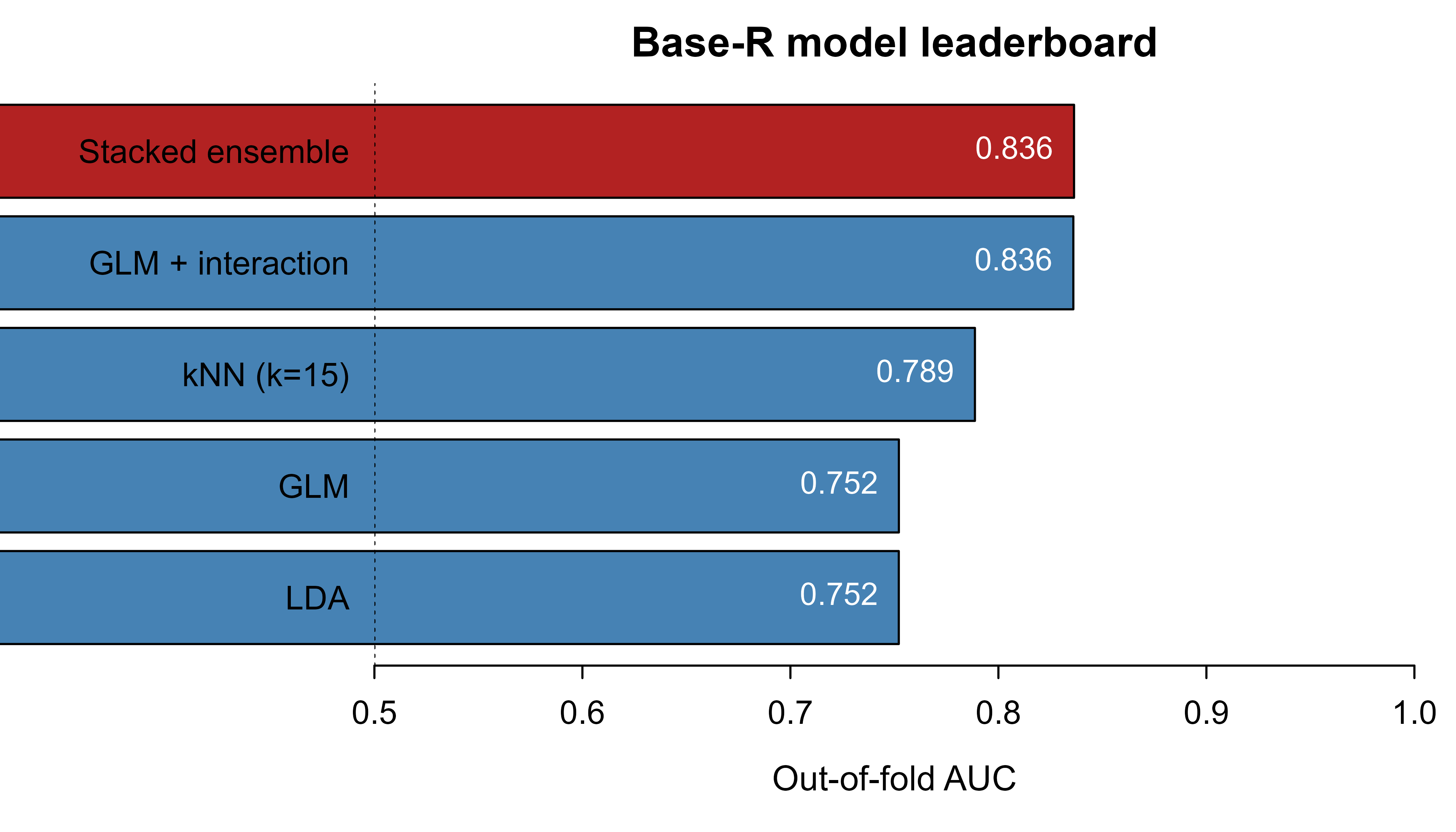

Figure 97.1: Out-of-fold AUC for each model family in the base-R leaderboard. Higher is better.

The takeaways carry over directly to h2o.automl(): honest comparison needs out-of-fold predictions, a stacked ensemble usually edges out its best base model, and the gain over a well-specified single model can be small enough that serving cost decides which to deploy.

97.7 Practical guidance, pitfalls, and when to use it

Reach for h2o when at least one of these holds: the data is too large for R’s memory, you want a strong tabular baseline from one h2o.automl() call, or you need a scoring artifact (MOJO/POJO) that runs on a JVM without R. For small data that fits in memory and a workflow you want full control over, tidymodels with the engines in this book is usually a better fit, and for boosting specifically, calling xgboost or lightgbm directly avoids the cluster overhead.

Recurring pitfalls:

• Forgetting the response factor. For classification the response column must be a factor in the cluster (as.factor); a numeric 0/1 response makes h2o fit a regression and silently report regression metrics.
• Cluster memory leaks. Frames and models persist in the JVM. Long sessions exhaust the heap; call h2o.rm() on intermediates or h2o.removeAll() between experiments.
• Version skew. The R h2o package and the running cluster must be the same version. Reinstall the client when you upgrade the cluster.
• Reading too much into AutoML accuracy. The leaderboard optimizes one metric on cross-validation; always confirm on a truly held-out frame and weigh ensemble accuracy against serving cost.
• Set a seed and a reproducibility mode. Distributed training is only reproducible when you fix seed and, for deep learning, set reproducible = TRUE (which forces single-threaded training and is slow).
• Leakage through preprocessing. If you impute or encode in R before as.h2o, do it on training rows only. Better, let h2o handle missing values and high-cardinality factors natively inside cross-validation.

97.8 Further reading

• Hastie, Tibshirian, and Friedman (2009), The Elements of Statistical Learning, for the GLM, boosting, random forest, and stacking theory the h2o algorithms implement.
• Friedman (2001), “Greedy Function Approximation: A Gradient Boosting Machine,” for the gradient boosting derivation.
• Breiman (2001), “Random Forests,” for the bagging-plus-feature-subsampling argument.
• Wolpert (1992), “Stacked Generalization,” and van der Laan, Polley, and Hubbard (2007), “Super Learner,” for the out-of-fold stacking that AutoML’s ensembles use.
• LeDell and Poirier (2020), “H2O AutoML: Scalable Automatic Machine Learning,” for the design of h2o.automl.
• Molnar (2022), Interpretable Machine Learning, for partial dependence and SHAP, the explainability tools exposed by h2o.explain().
• The H2O.ai documentation and R package vignettes for current arguments, defaults, and the MOJO/POJO export workflow.

:::{#quarto-navigation-envelope .hidden}
[Advanced Data Analysis]{.hidden .quarto-markdown-envelope-contents render-id="cXVhcnRvLWludC1zaWRlYmFyLXRpdGxl"}
[Advanced Data Analysis]{.hidden .quarto-markdown-envelope-contents render-id="cXVhcnRvLWludC1uYXZiYXItdGl0bGU="}
[<span class='chapter-number'>98</span>  <span class='chapter-title'>Automated Machine Learning (AutoML)</span>]{.hidden .quarto-markdown-envelope-contents render-id="cXVhcnRvLWludC1uZXh0"}
[<span class='chapter-number'>96</span>  <span class='chapter-title'>Distributed Machine Learning with Spark and sparklyr</span>]{.hidden .quarto-markdown-envelope-contents render-id="cXVhcnRvLWludC1wcmV2"}
[Preface]{.hidden .quarto-markdown-envelope-contents render-id="cXVhcnRvLWludC1zaWRlYmFyOi9pbmRleC5odG1sUHJlZmFjZQ=="}
[Machine Learning]{.hidden .quarto-markdown-envelope-contents render-id="cXVhcnRvLWludC1zaWRlYmFyOnF1YXJ0by1zaWRlYmFyLXNlY3Rpb24tMQ=="}
[<span class='chapter-number'>1</span>  <span class='chapter-title'>Introduction</span>]{.hidden .quarto-markdown-envelope-contents render-id="cXVhcnRvLWludC1zaWRlYmFyOi8wMDItaW50cm8uaHRtbDxzcGFuLWNsYXNzPSdjaGFwdGVyLW51bWJlcic+MTwvc3Bhbj4tLTxzcGFuLWNsYXNzPSdjaGFwdGVyLXRpdGxlJz5JbnRyb2R1Y3Rpb248L3NwYW4+"}
[<span class='chapter-number'>2</span>  <span class='chapter-title'>Overview of Learning Paradigms</span>]{.hidden .quarto-markdown-envelope-contents render-id="cXVhcnRvLWludC1zaWRlYmFyOi8wMDMtb3ZlcnZpZXcuaHRtbDxzcGFuLWNsYXNzPSdjaGFwdGVyLW51bWJlcic+Mjwvc3Bhbj4tLTxzcGFuLWNsYXNzPSdjaGFwdGVyLXRpdGxlJz5PdmVydmlldy1vZi1MZWFybmluZy1QYXJhZGlnbXM8L3NwYW4+"}
[Supervised Learning: Local-Based Methods]{.hidden .quarto-markdown-envelope-contents render-id="cXVhcnRvLWludC1zaWRlYmFyOnF1YXJ0by1zaWRlYmFyLXNlY3Rpb24tMg=="}
[<span class='chapter-number'>3</span>  <span class='chapter-title'>Spline Regression</span>]{.hidden .quarto-markdown-envelope-contents render-id="cXVhcnRvLWludC1zaWRlYmFyOi8wMDUtc3BsaW5lLmh0bWw8c3Bhbi1jbGFzcz0nY2hhcHRlci1udW1iZXInPjM8L3NwYW4+LS08c3Bhbi1jbGFzcz0nY2hhcHRlci10aXRsZSc+U3BsaW5lLVJlZ3Jlc3Npb248L3NwYW4+"}
[<span class='chapter-number'>4</span>  <span class='chapter-title'>Kernel Smoothing</span>]{.hidden .quarto-markdown-envelope-contents render-id="cXVhcnRvLWludC1zaWRlYmFyOi8wMDYta2VybmVsLmh0bWw8c3Bhbi1jbGFzcz0nY2hhcHRlci1udW1iZXInPjQ8L3NwYW4+LS08c3Bhbi1jbGFzcz0nY2hhcHRlci10aXRsZSc+S2VybmVsLVNtb290aGluZzwvc3Bhbj4="}
[<span class='chapter-number'>5</span>  <span class='chapter-title'>Local Regression</span>]{.hidden .quarto-markdown-envelope-contents render-id="cXVhcnRvLWludC1zaWRlYmFyOi8wMDctbG9jYWwuaHRtbDxzcGFuLWNsYXNzPSdjaGFwdGVyLW51bWJlcic+NTwvc3Bhbj4tLTxzcGFuLWNsYXNzPSdjaGFwdGVyLXRpdGxlJz5Mb2NhbC1SZWdyZXNzaW9uPC9zcGFuPg=="}
[Supervised Learning: Transformation-Based Methods]{.hidden .quarto-markdown-envelope-contents render-id="cXVhcnRvLWludC1zaWRlYmFyOnF1YXJ0by1zaWRlYmFyLXNlY3Rpb24tMw=="}
[<span class='chapter-number'>6</span>  <span class='chapter-title'>Generalized Additive Models</span>]{.hidden .quarto-markdown-envelope-contents render-id="cXVhcnRvLWludC1zaWRlYmFyOi8wMDktZ2FtLmh0bWw8c3Bhbi1jbGFzcz0nY2hhcHRlci1udW1iZXInPjY8L3NwYW4+LS08c3Bhbi1jbGFzcz0nY2hhcHRlci10aXRsZSc+R2VuZXJhbGl6ZWQtQWRkaXRpdmUtTW9kZWxzPC9zcGFuPg=="}
[<span class='chapter-number'>7</span>  <span class='chapter-title'>Gaussian Process Regression</span>]{.hidden .quarto-markdown-envelope-contents render-id="cXVhcnRvLWludC1zaWRlYmFyOi8wMTAtZ2F1c3NpYW4tcHJvY2Vzcy1yZWcuaHRtbDxzcGFuLWNsYXNzPSdjaGFwdGVyLW51bWJlcic+Nzwvc3Bhbj4tLTxzcGFuLWNsYXNzPSdjaGFwdGVyLXRpdGxlJz5HYXVzc2lhbi1Qcm9jZXNzLVJlZ3Jlc3Npb248L3NwYW4+"}
[Supervised Learning: Tree-Based Methods]{.hidden .quarto-markdown-envelope-contents render-id="cXVhcnRvLWludC1zaWRlYmFyOnF1YXJ0by1zaWRlYmFyLXNlY3Rpb24tNA=="}
[<span class='chapter-number'>8</span>  <span class='chapter-title'>Classification and Regression Trees</span>]{.hidden .quarto-markdown-envelope-contents render-id="cXVhcnRvLWludC1zaWRlYmFyOi8wMTItcmVncmVzc2lvbi10cmVlcy5odG1sPHNwYW4tY2xhc3M9J2NoYXB0ZXItbnVtYmVyJz44PC9zcGFuPi0tPHNwYW4tY2xhc3M9J2NoYXB0ZXItdGl0bGUnPkNsYXNzaWZpY2F0aW9uLWFuZC1SZWdyZXNzaW9uLVRyZWVzPC9zcGFuPg=="}
[<span class='chapter-number'>9</span>  <span class='chapter-title'>Multivariate Adaptive Regression Splines</span>]{.hidden .quarto-markdown-envelope-contents render-id="cXVhcnRvLWludC1zaWRlYmFyOi8wMTMtTUFSUy5odG1sPHNwYW4tY2xhc3M9J2NoYXB0ZXItbnVtYmVyJz45PC9zcGFuPi0tPHNwYW4tY2xhc3M9J2NoYXB0ZXItdGl0bGUnPk11bHRpdmFyaWF0ZS1BZGFwdGl2ZS1SZWdyZXNzaW9uLVNwbGluZXM8L3NwYW4+"}
[<span class='chapter-number'>10</span>  <span class='chapter-title'>Bagging</span>]{.hidden .quarto-markdown-envelope-contents render-id="cXVhcnRvLWludC1zaWRlYmFyOi8wMTQtYmFnZ2luZy5odG1sPHNwYW4tY2xhc3M9J2NoYXB0ZXItbnVtYmVyJz4xMDwvc3Bhbj4tLTxzcGFuLWNsYXNzPSdjaGFwdGVyLXRpdGxlJz5CYWdnaW5nPC9zcGFuPg=="}
[<span class='chapter-number'>11</span>  <span class='chapter-title'>Boosting</span>]{.hidden .quarto-markdown-envelope-contents render-id="cXVhcnRvLWludC1zaWRlYmFyOi8wMTUtYm9vc3RpbmcuaHRtbDxzcGFuLWNsYXNzPSdjaGFwdGVyLW51bWJlcic+MTE8L3NwYW4+LS08c3Bhbi1jbGFzcz0nY2hhcHRlci10aXRsZSc+Qm9vc3Rpbmc8L3NwYW4+"}
[<span class='chapter-number'>12</span>  <span class='chapter-title'>Gradient Boosting in Practice</span>]{.hidden .quarto-markdown-envelope-contents render-id="cXVhcnRvLWludC1zaWRlYmFyOi8wMTYtZ3JhZGllbnQtYm9vc3RpbmcuaHRtbDxzcGFuLWNsYXNzPSdjaGFwdGVyLW51bWJlcic+MTI8L3NwYW4+LS08c3Bhbi1jbGFzcz0nY2hhcHRlci10aXRsZSc+R3JhZGllbnQtQm9vc3RpbmctaW4tUHJhY3RpY2U8L3NwYW4+"}
[<span class='chapter-number'>13</span>  <span class='chapter-title'>Random Forests</span>]{.hidden .quarto-markdown-envelope-contents render-id="cXVhcnRvLWludC1zaWRlYmFyOi8wMTctcmFuZG9tLWZvcmVzdC5odG1sPHNwYW4tY2xhc3M9J2NoYXB0ZXItbnVtYmVyJz4xMzwvc3Bhbj4tLTxzcGFuLWNsYXNzPSdjaGFwdGVyLXRpdGxlJz5SYW5kb20tRm9yZXN0czwvc3Bhbj4="}
[<span class='chapter-number'>14</span>  <span class='chapter-title'>Bayesian Additive Regression Trees</span>]{.hidden .quarto-markdown-envelope-contents render-id="cXVhcnRvLWludC1zaWRlYmFyOi8wMTgtQkFSVC5odG1sPHNwYW4tY2xhc3M9J2NoYXB0ZXItbnVtYmVyJz4xNDwvc3Bhbj4tLTxzcGFuLWNsYXNzPSdjaGFwdGVyLXRpdGxlJz5CYXllc2lhbi1BZGRpdGl2ZS1SZWdyZXNzaW9uLVRyZWVzPC9zcGFuPg=="}
[Supervised Learning: Neural Networks]{.hidden .quarto-markdown-envelope-contents render-id="cXVhcnRvLWludC1zaWRlYmFyOnF1YXJ0by1zaWRlYmFyLXNlY3Rpb24tNQ=="}
[<span class='chapter-number'>15</span>  <span class='chapter-title'>Neural Networks</span>]{.hidden .quarto-markdown-envelope-contents render-id="cXVhcnRvLWludC1zaWRlYmFyOi8wMjAtbmV1cmFsLW5ldHdvcmtzLmh0bWw8c3Bhbi1jbGFzcz0nY2hhcHRlci1udW1iZXInPjE1PC9zcGFuPi0tPHNwYW4tY2xhc3M9J2NoYXB0ZXItdGl0bGUnPk5ldXJhbC1OZXR3b3Jrczwvc3Bhbj4="}
[<span class='chapter-number'>16</span>  <span class='chapter-title'>Artificial Intelligence</span>]{.hidden .quarto-markdown-envelope-contents render-id="cXVhcnRvLWludC1zaWRlYmFyOi8wMjEtQUkuaHRtbDxzcGFuLWNsYXNzPSdjaGFwdGVyLW51bWJlcic+MTY8L3NwYW4+LS08c3Bhbi1jbGFzcz0nY2hhcHRlci10aXRsZSc+QXJ0aWZpY2lhbC1JbnRlbGxpZ2VuY2U8L3NwYW4+"}
[Supervised Learning: Other Methods]{.hidden .quarto-markdown-envelope-contents render-id="cXVhcnRvLWludC1zaWRlYmFyOnF1YXJ0by1zaWRlYmFyLXNlY3Rpb24tNg=="}
[<span class='chapter-number'>17</span>  <span class='chapter-title'>k-Nearest Neighbors</span>]{.hidden .quarto-markdown-envelope-contents render-id="cXVhcnRvLWludC1zaWRlYmFyOi8wMjMta25uLmh0bWw8c3Bhbi1jbGFzcz0nY2hhcHRlci1udW1iZXInPjE3PC9zcGFuPi0tPHNwYW4tY2xhc3M9J2NoYXB0ZXItdGl0bGUnPmstTmVhcmVzdC1OZWlnaGJvcnM8L3NwYW4+"}
[<span class='chapter-number'>18</span>  <span class='chapter-title'>Naive Bayes</span>]{.hidden .quarto-markdown-envelope-contents render-id="cXVhcnRvLWludC1zaWRlYmFyOi8wMjQtbmFpdmUtYmF5ZXMuaHRtbDxzcGFuLWNsYXNzPSdjaGFwdGVyLW51bWJlcic+MTg8L3NwYW4+LS08c3Bhbi1jbGFzcz0nY2hhcHRlci10aXRsZSc+TmFpdmUtQmF5ZXM8L3NwYW4+"}
[<span class='chapter-number'>19</span>  <span class='chapter-title'>Support Vector</span>]{.hidden .quarto-markdown-envelope-contents render-id="cXVhcnRvLWludC1zaWRlYmFyOi8wMjUtc3ZtLmh0bWw8c3Bhbi1jbGFzcz0nY2hhcHRlci1udW1iZXInPjE5PC9zcGFuPi0tPHNwYW4tY2xhc3M9J2NoYXB0ZXItdGl0bGUnPlN1cHBvcnQtVmVjdG9yPC9zcGFuPg=="}
[<span class='chapter-number'>20</span>  <span class='chapter-title'>Discriminant Analysis</span>]{.hidden .quarto-markdown-envelope-contents render-id="cXVhcnRvLWludC1zaWRlYmFyOi8wMjYtZGlzY3JpbWluYW50LWFuYWx5c2lzLmh0bWw8c3Bhbi1jbGFzcz0nY2hhcHRlci1udW1iZXInPjIwPC9zcGFuPi0tPHNwYW4tY2xhc3M9J2NoYXB0ZXItdGl0bGUnPkRpc2NyaW1pbmFudC1BbmFseXNpczwvc3Bhbj4="}
[<span class='chapter-number'>21</span>  <span class='chapter-title'>Quantile Regression</span>]{.hidden .quarto-markdown-envelope-contents render-id="cXVhcnRvLWludC1zaWRlYmFyOi8wMjctcXVhbnRpbGUtcmVnLmh0bWw8c3Bhbi1jbGFzcz0nY2hhcHRlci1udW1iZXInPjIxPC9zcGFuPi0tPHNwYW4tY2xhc3M9J2NoYXB0ZXItdGl0bGUnPlF1YW50aWxlLVJlZ3Jlc3Npb248L3NwYW4+"}
[Unsupervised Learning: Clustering]{.hidden .quarto-markdown-envelope-contents render-id="cXVhcnRvLWludC1zaWRlYmFyOnF1YXJ0by1zaWRlYmFyLXNlY3Rpb24tNw=="}
[<span class='chapter-number'>22</span>  <span class='chapter-title'>Introduction</span>]{.hidden .quarto-markdown-envelope-contents render-id="cXVhcnRvLWludC1zaWRlYmFyOi8wMjktaW50cm8tdW5zdXBlcnZpc2VkLmh0bWw8c3Bhbi1jbGFzcz0nY2hhcHRlci1udW1iZXInPjIyPC9zcGFuPi0tPHNwYW4tY2xhc3M9J2NoYXB0ZXItdGl0bGUnPkludHJvZHVjdGlvbjwvc3Bhbj4="}
[<span class='chapter-number'>23</span>  <span class='chapter-title'>Cluster Analysis</span>]{.hidden .quarto-markdown-envelope-contents render-id="cXVhcnRvLWludC1zaWRlYmFyOi8wMzAtY2x1c3Rlci5odG1sPHNwYW4tY2xhc3M9J2NoYXB0ZXItbnVtYmVyJz4yMzwvc3Bhbj4tLTxzcGFuLWNsYXNzPSdjaGFwdGVyLXRpdGxlJz5DbHVzdGVyLUFuYWx5c2lzPC9zcGFuPg=="}
[<span class='chapter-number'>24</span>  <span class='chapter-title'>Gaussian Mixture Models and the EM Algorithm</span>]{.hidden .quarto-markdown-envelope-contents render-id="cXVhcnRvLWludC1zaWRlYmFyOi8wMzBhLWdtbS1lbS5odG1sPHNwYW4tY2xhc3M9J2NoYXB0ZXItbnVtYmVyJz4yNDwvc3Bhbj4tLTxzcGFuLWNsYXNzPSdjaGFwdGVyLXRpdGxlJz5HYXVzc2lhbi1NaXh0dXJlLU1vZGVscy1hbmQtdGhlLUVNLUFsZ29yaXRobTwvc3Bhbj4="}
[<span class='chapter-number'>25</span>  <span class='chapter-title'>Spectral Clustering</span>]{.hidden .quarto-markdown-envelope-contents render-id="cXVhcnRvLWludC1zaWRlYmFyOi8wMzBiLXNwZWN0cmFsLWNsdXN0ZXJpbmcuaHRtbDxzcGFuLWNsYXNzPSdjaGFwdGVyLW51bWJlcic+MjU8L3NwYW4+LS08c3Bhbi1jbGFzcz0nY2hhcHRlci10aXRsZSc+U3BlY3RyYWwtQ2x1c3RlcmluZzwvc3Bhbj4="}
[<span class='chapter-number'>26</span>  <span class='chapter-title'>Self-Organizing Maps</span>]{.hidden .quarto-markdown-envelope-contents render-id="cXVhcnRvLWludC1zaWRlYmFyOi8wMzBjLXNlbGYtb3JnYW5pemluZy1tYXBzLmh0bWw8c3Bhbi1jbGFzcz0nY2hhcHRlci1udW1iZXInPjI2PC9zcGFuPi0tPHNwYW4tY2xhc3M9J2NoYXB0ZXItdGl0bGUnPlNlbGYtT3JnYW5pemluZy1NYXBzPC9zcGFuPg=="}
[Unsupervised Learning: Dimension Reduction and Representation]{.hidden .quarto-markdown-envelope-contents render-id="cXVhcnRvLWludC1zaWRlYmFyOnF1YXJ0by1zaWRlYmFyLXNlY3Rpb24tOA=="}
[<span class='chapter-number'>27</span>  <span class='chapter-title'>Dimension Reduction</span>]{.hidden .quarto-markdown-envelope-contents render-id="cXVhcnRvLWludC1zaWRlYmFyOi8wMzEtZGltZW5zaW9uLXJlZHVjdGlvbi5odG1sPHNwYW4tY2xhc3M9J2NoYXB0ZXItbnVtYmVyJz4yNzwvc3Bhbj4tLTxzcGFuLWNsYXNzPSdjaGFwdGVyLXRpdGxlJz5EaW1lbnNpb24tUmVkdWN0aW9uPC9zcGFuPg=="}
[<span class='chapter-number'>28</span>  <span class='chapter-title'>Independent Component Analysis</span>]{.hidden .quarto-markdown-envelope-contents render-id="cXVhcnRvLWludC1zaWRlYmFyOi8wMzFhLWljYS5odG1sPHNwYW4tY2xhc3M9J2NoYXB0ZXItbnVtYmVyJz4yODwvc3Bhbj4tLTxzcGFuLWNsYXNzPSdjaGFwdGVyLXRpdGxlJz5JbmRlcGVuZGVudC1Db21wb25lbnQtQW5hbHlzaXM8L3NwYW4+"}
[<span class='chapter-number'>29</span>  <span class='chapter-title'>Non-negative Matrix Factorization</span>]{.hidden .quarto-markdown-envelope-contents render-id="cXVhcnRvLWludC1zaWRlYmFyOi8wMzFiLW5tZi5odG1sPHNwYW4tY2xhc3M9J2NoYXB0ZXItbnVtYmVyJz4yOTwvc3Bhbj4tLTxzcGFuLWNsYXNzPSdjaGFwdGVyLXRpdGxlJz5Ob24tbmVnYXRpdmUtTWF0cml4LUZhY3Rvcml6YXRpb248L3NwYW4+"}
[<span class='chapter-number'>30</span>  <span class='chapter-title'>Factor Analysis</span>]{.hidden .quarto-markdown-envelope-contents render-id="cXVhcnRvLWludC1zaWRlYmFyOi8wMzFjLWZhY3Rvci1hbmFseXNpcy5odG1sPHNwYW4tY2xhc3M9J2NoYXB0ZXItbnVtYmVyJz4zMDwvc3Bhbj4tLTxzcGFuLWNsYXNzPSdjaGFwdGVyLXRpdGxlJz5GYWN0b3ItQW5hbHlzaXM8L3NwYW4+"}
[<span class='chapter-number'>31</span>  <span class='chapter-title'>Multidimensional Scaling and Nonlinear Dimension Reduction</span>]{.hidden .quarto-markdown-envelope-contents render-id="cXVhcnRvLWludC1zaWRlYmFyOi8wMzItc2NhbGluZy5odG1sPHNwYW4tY2xhc3M9J2NoYXB0ZXItbnVtYmVyJz4zMTwvc3Bhbj4tLTxzcGFuLWNsYXNzPSdjaGFwdGVyLXRpdGxlJz5NdWx0aWRpbWVuc2lvbmFsLVNjYWxpbmctYW5kLU5vbmxpbmVhci1EaW1lbnNpb24tUmVkdWN0aW9uPC9zcGFuPg=="}
[Unsupervised Learning: Density, Patterns, and Interpretability]{.hidden .quarto-markdown-envelope-contents render-id="cXVhcnRvLWludC1zaWRlYmFyOnF1YXJ0by1zaWRlYmFyLXNlY3Rpb24tOQ=="}
[<span class='chapter-number'>32</span>  <span class='chapter-title'>Density Estimation</span>]{.hidden .quarto-markdown-envelope-contents render-id="cXVhcnRvLWludC1zaWRlYmFyOi8wMzQtZGVuc2l0eS1lc3RpbWF0aW9uLmh0bWw8c3Bhbi1jbGFzcz0nY2hhcHRlci1udW1iZXInPjMyPC9zcGFuPi0tPHNwYW4tY2xhc3M9J2NoYXB0ZXItdGl0bGUnPkRlbnNpdHktRXN0aW1hdGlvbjwvc3Bhbj4="}
[<span class='chapter-number'>33</span>  <span class='chapter-title'>Association Rule Mining</span>]{.hidden .quarto-markdown-envelope-contents render-id="cXVhcnRvLWludC1zaWRlYmFyOi8wMzNhLWFzc29jaWF0aW9uLXJ1bGVzLmh0bWw8c3Bhbi1jbGFzcz0nY2hhcHRlci1udW1iZXInPjMzPC9zcGFuPi0tPHNwYW4tY2xhc3M9J2NoYXB0ZXItdGl0bGUnPkFzc29jaWF0aW9uLVJ1bGUtTWluaW5nPC9zcGFuPg=="}
[<span class='chapter-number'>34</span>  <span class='chapter-title'>Topic Models and Latent Dirichlet Allocation</span>]{.hidden .quarto-markdown-envelope-contents render-id="cXVhcnRvLWludC1zaWRlYmFyOi8wMzNiLXRvcGljLW1vZGVscy5odG1sPHNwYW4tY2xhc3M9J2NoYXB0ZXItbnVtYmVyJz4zNDwvc3Bhbj4tLTxzcGFuLWNsYXNzPSdjaGFwdGVyLXRpdGxlJz5Ub3BpYy1Nb2RlbHMtYW5kLUxhdGVudC1EaXJpY2hsZXQtQWxsb2NhdGlvbjwvc3Bhbj4="}
[<span class='chapter-number'>35</span>  <span class='chapter-title'>Interpretable Machine Learning</span>]{.hidden .quarto-markdown-envelope-contents render-id="cXVhcnRvLWludC1zaWRlYmFyOi8wMzMtaW50ZXJwcmV0YWJsZS1tYWNoaW5lLWxlYXJuaW5nLmh0bWw8c3Bhbi1jbGFzcz0nY2hhcHRlci1udW1iZXInPjM1PC9zcGFuPi0tPHNwYW4tY2xhc3M9J2NoYXB0ZXItdGl0bGUnPkludGVycHJldGFibGUtTWFjaGluZS1MZWFybmluZzwvc3Bhbj4="}
[Deep Learning]{.hidden .quarto-markdown-envelope-contents render-id="cXVhcnRvLWludC1zaWRlYmFyOnF1YXJ0by1zaWRlYmFyLXNlY3Rpb24tMTA="}
[<span class='chapter-number'>36</span>  <span class='chapter-title'>Convolutional Neural Networks</span>]{.hidden .quarto-markdown-envelope-contents render-id="cXVhcnRvLWludC1zaWRlYmFyOi8wMzVhLWNubi5odG1sPHNwYW4tY2xhc3M9J2NoYXB0ZXItbnVtYmVyJz4zNjwvc3Bhbj4tLTxzcGFuLWNsYXNzPSdjaGFwdGVyLXRpdGxlJz5Db252b2x1dGlvbmFsLU5ldXJhbC1OZXR3b3Jrczwvc3Bhbj4="}
[<span class='chapter-number'>37</span>  <span class='chapter-title'>Recurrent Neural Networks: LSTMs and GRUs</span>]{.hidden .quarto-markdown-envelope-contents render-id="cXVhcnRvLWludC1zaWRlYmFyOi8wMzViLXJubi5odG1sPHNwYW4tY2xhc3M9J2NoYXB0ZXItbnVtYmVyJz4zNzwvc3Bhbj4tLTxzcGFuLWNsYXNzPSdjaGFwdGVyLXRpdGxlJz5SZWN1cnJlbnQtTmV1cmFsLU5ldHdvcmtzOi1MU1RNcy1hbmQtR1JVczwvc3Bhbj4="}
[<span class='chapter-number'>38</span>  <span class='chapter-title'>Attention and Transformers</span>]{.hidden .quarto-markdown-envelope-contents render-id="cXVhcnRvLWludC1zaWRlYmFyOi8wMzYtdHJhbnNmb3JtZXJzLmh0bWw8c3Bhbi1jbGFzcz0nY2hhcHRlci1udW1iZXInPjM4PC9zcGFuPi0tPHNwYW4tY2xhc3M9J2NoYXB0ZXItdGl0bGUnPkF0dGVudGlvbi1hbmQtVHJhbnNmb3JtZXJzPC9zcGFuPg=="}
[<span class='chapter-number'>39</span>  <span class='chapter-title'>BERT</span>]{.hidden .quarto-markdown-envelope-contents render-id="cXVhcnRvLWludC1zaWRlYmFyOi8wMzctQkVSVC5odG1sPHNwYW4tY2xhc3M9J2NoYXB0ZXItbnVtYmVyJz4zOTwvc3Bhbj4tLTxzcGFuLWNsYXNzPSdjaGFwdGVyLXRpdGxlJz5CRVJUPC9zcGFuPg=="}
[<span class='chapter-number'>40</span>  <span class='chapter-title'>Large Language Models and Foundation Models</span>]{.hidden .quarto-markdown-envelope-contents render-id="cXVhcnRvLWludC1zaWRlYmFyOi8wMzgtbGxtcy5odG1sPHNwYW4tY2xhc3M9J2NoYXB0ZXItbnVtYmVyJz40MDwvc3Bhbj4tLTxzcGFuLWNsYXNzPSdjaGFwdGVyLXRpdGxlJz5MYXJnZS1MYW5ndWFnZS1Nb2RlbHMtYW5kLUZvdW5kYXRpb24tTW9kZWxzPC9zcGFuPg=="}
[<span class='chapter-number'>41</span>  <span class='chapter-title'>Autoencoders and Representation Learning</span>]{.hidden .quarto-markdown-envelope-contents render-id="cXVhcnRvLWludC1zaWRlYmFyOi8wMzktYXV0b2VuY29kZXJzLmh0bWw8c3Bhbi1jbGFzcz0nY2hhcHRlci1udW1iZXInPjQxPC9zcGFuPi0tPHNwYW4tY2xhc3M9J2NoYXB0ZXItdGl0bGUnPkF1dG9lbmNvZGVycy1hbmQtUmVwcmVzZW50YXRpb24tTGVhcm5pbmc8L3NwYW4+"}
[<span class='chapter-number'>42</span>  <span class='chapter-title'>Generative Models</span>]{.hidden .quarto-markdown-envelope-contents render-id="cXVhcnRvLWludC1zaWRlYmFyOi8wNDAtZ2VuZXJhdGl2ZS1tb2RlbHMuaHRtbDxzcGFuLWNsYXNzPSdjaGFwdGVyLW51bWJlcic+NDI8L3NwYW4+LS08c3Bhbi1jbGFzcz0nY2hhcHRlci10aXRsZSc+R2VuZXJhdGl2ZS1Nb2RlbHM8L3NwYW4+"}
[<span class='chapter-number'>43</span>  <span class='chapter-title'>Diffusion Models</span>]{.hidden .quarto-markdown-envelope-contents render-id="cXVhcnRvLWludC1zaWRlYmFyOi8wNDBhLWRpZmZ1c2lvbi5odG1sPHNwYW4tY2xhc3M9J2NoYXB0ZXItbnVtYmVyJz40Mzwvc3Bhbj4tLTxzcGFuLWNsYXNzPSdjaGFwdGVyLXRpdGxlJz5EaWZmdXNpb24tTW9kZWxzPC9zcGFuPg=="}
[<span class='chapter-number'>44</span>  <span class='chapter-title'>Graph Neural Networks</span>]{.hidden .quarto-markdown-envelope-contents render-id="cXVhcnRvLWludC1zaWRlYmFyOi8wNDEtZ3JhcGgtbmV1cmFsLW5ldHdvcmtzLmh0bWw8c3Bhbi1jbGFzcz0nY2hhcHRlci1udW1iZXInPjQ0PC9zcGFuPi0tPHNwYW4tY2xhc3M9J2NoYXB0ZXItdGl0bGUnPkdyYXBoLU5ldXJhbC1OZXR3b3Jrczwvc3Bhbj4="}
[<span class='chapter-number'>45</span>  <span class='chapter-title'>Mixture of Experts and Conditional Computation</span>]{.hidden .quarto-markdown-envelope-contents render-id="cXVhcnRvLWludC1zaWRlYmFyOi8wNDItbWl4dHVyZS1vZi1leHBlcnRzLmh0bWw8c3Bhbi1jbGFzcz0nY2hhcHRlci1udW1iZXInPjQ1PC9zcGFuPi0tPHNwYW4tY2xhc3M9J2NoYXB0ZXItdGl0bGUnPk1peHR1cmUtb2YtRXhwZXJ0cy1hbmQtQ29uZGl0aW9uYWwtQ29tcHV0YXRpb248L3NwYW4+"}
[<span class='chapter-number'>46</span>  <span class='chapter-title'>Bayesian Deep Learning and Uncertainty Quantification</span>]{.hidden .quarto-markdown-envelope-contents render-id="cXVhcnRvLWludC1zaWRlYmFyOi8wNDMtYmF5ZXNpYW4tZGVlcC1sZWFybmluZy5odG1sPHNwYW4tY2xhc3M9J2NoYXB0ZXItbnVtYmVyJz40Njwvc3Bhbj4tLTxzcGFuLWNsYXNzPSdjaGFwdGVyLXRpdGxlJz5CYXllc2lhbi1EZWVwLUxlYXJuaW5nLWFuZC1VbmNlcnRhaW50eS1RdWFudGlmaWNhdGlvbjwvc3Bhbj4="}
[<span class='chapter-number'>47</span>  <span class='chapter-title'>Double Descent</span>]{.hidden .quarto-markdown-envelope-contents render-id="cXVhcnRvLWludC1zaWRlYmFyOi8wNDNiLWRvdWJsZS1kZXNjZW50Lmh0bWw8c3Bhbi1jbGFzcz0nY2hhcHRlci1udW1iZXInPjQ3PC9zcGFuPi0tPHNwYW4tY2xhc3M9J2NoYXB0ZXItdGl0bGUnPkRvdWJsZS1EZXNjZW50PC9zcGFuPg=="}
[Learning Paradigms]{.hidden .quarto-markdown-envelope-contents render-id="cXVhcnRvLWludC1zaWRlYmFyOnF1YXJ0by1zaWRlYmFyLXNlY3Rpb24tMTE="}
[<span class='chapter-number'>48</span>  <span class='chapter-title'>Semi-Supervised Learning</span>]{.hidden .quarto-markdown-envelope-contents render-id="cXVhcnRvLWludC1zaWRlYmFyOi8wNDUtc2VtaS1zdXBlcnZpc2VkLWxlYXJuaW5nLmh0bWw8c3Bhbi1jbGFzcz0nY2hhcHRlci1udW1iZXInPjQ4PC9zcGFuPi0tPHNwYW4tY2xhc3M9J2NoYXB0ZXItdGl0bGUnPlNlbWktU3VwZXJ2aXNlZC1MZWFybmluZzwvc3Bhbj4="}
[<span class='chapter-number'>49</span>  <span class='chapter-title'>Self-Supervised and Contrastive Learning</span>]{.hidden .quarto-markdown-envelope-contents render-id="cXVhcnRvLWludC1zaWRlYmFyOi8wNDYtc2VsZi1zdXBlcnZpc2VkLWxlYXJuaW5nLmh0bWw8c3Bhbi1jbGFzcz0nY2hhcHRlci1udW1iZXInPjQ5PC9zcGFuPi0tPHNwYW4tY2xhc3M9J2NoYXB0ZXItdGl0bGUnPlNlbGYtU3VwZXJ2aXNlZC1hbmQtQ29udHJhc3RpdmUtTGVhcm5pbmc8L3NwYW4+"}
[<span class='chapter-number'>50</span>  <span class='chapter-title'>Active Learning</span>]{.hidden .quarto-markdown-envelope-contents render-id="cXVhcnRvLWludC1zaWRlYmFyOi8wNDctYWN0aXZlLWxlYXJuaW5nLmh0bWw8c3Bhbi1jbGFzcz0nY2hhcHRlci1udW1iZXInPjUwPC9zcGFuPi0tPHNwYW4tY2xhc3M9J2NoYXB0ZXItdGl0bGUnPkFjdGl2ZS1MZWFybmluZzwvc3Bhbj4="}
[<span class='chapter-number'>51</span>  <span class='chapter-title'>Weakly-Supervised and Positive-Unlabeled Learning</span>]{.hidden .quarto-markdown-envelope-contents render-id="cXVhcnRvLWludC1zaWRlYmFyOi8wNDgtd2Vha2x5LXN1cGVydmlzZWQtcHUuaHRtbDxzcGFuLWNsYXNzPSdjaGFwdGVyLW51bWJlcic+NTE8L3NwYW4+LS08c3Bhbi1jbGFzcz0nY2hhcHRlci10aXRsZSc+V2Vha2x5LVN1cGVydmlzZWQtYW5kLVBvc2l0aXZlLVVubGFiZWxlZC1MZWFybmluZzwvc3Bhbj4="}
[<span class='chapter-number'>52</span>  <span class='chapter-title'>Few-Shot and Zero-Shot Learning</span>]{.hidden .quarto-markdown-envelope-contents render-id="cXVhcnRvLWludC1zaWRlYmFyOi8wNDktZmV3LXNob3QtemVyby1zaG90Lmh0bWw8c3Bhbi1jbGFzcz0nY2hhcHRlci1udW1iZXInPjUyPC9zcGFuPi0tPHNwYW4tY2xhc3M9J2NoYXB0ZXItdGl0bGUnPkZldy1TaG90LWFuZC1aZXJvLVNob3QtTGVhcm5pbmc8L3NwYW4+"}
[<span class='chapter-number'>53</span>  <span class='chapter-title'>Meta-Learning and Few-Shot Learning</span>]{.hidden .quarto-markdown-envelope-contents render-id="cXVhcnRvLWludC1zaWRlYmFyOi8wNTAtbWV0YS1sZWFybmluZy5odG1sPHNwYW4tY2xhc3M9J2NoYXB0ZXItbnVtYmVyJz41Mzwvc3Bhbj4tLTxzcGFuLWNsYXNzPSdjaGFwdGVyLXRpdGxlJz5NZXRhLUxlYXJuaW5nLWFuZC1GZXctU2hvdC1MZWFybmluZzwvc3Bhbj4="}
[<span class='chapter-number'>54</span>  <span class='chapter-title'>Transfer and Multi-Task Learning</span>]{.hidden .quarto-markdown-envelope-contents render-id="cXVhcnRvLWludC1zaWRlYmFyOi8wNTEtdHJhbnNmZXItbXVsdGl0YXNrLWxlYXJuaW5nLmh0bWw8c3Bhbi1jbGFzcz0nY2hhcHRlci1udW1iZXInPjU0PC9zcGFuPi0tPHNwYW4tY2xhc3M9J2NoYXB0ZXItdGl0bGUnPlRyYW5zZmVyLWFuZC1NdWx0aS1UYXNrLUxlYXJuaW5nPC9zcGFuPg=="}
[<span class='chapter-number'>55</span>  <span class='chapter-title'>Online and Streaming Learning</span>]{.hidden .quarto-markdown-envelope-contents render-id="cXVhcnRvLWludC1zaWRlYmFyOi8wNTItb25saW5lLWxlYXJuaW5nLmh0bWw8c3Bhbi1jbGFzcz0nY2hhcHRlci1udW1iZXInPjU1PC9zcGFuPi0tPHNwYW4tY2xhc3M9J2NoYXB0ZXItdGl0bGUnPk9ubGluZS1hbmQtU3RyZWFtaW5nLUxlYXJuaW5nPC9zcGFuPg=="}
[<span class='chapter-number'>56</span>  <span class='chapter-title'>Federated Learning</span>]{.hidden .quarto-markdown-envelope-contents render-id="cXVhcnRvLWludC1zaWRlYmFyOi8wNTMtZmVkZXJhdGVkLWxlYXJuaW5nLmh0bWw8c3Bhbi1jbGFzcz0nY2hhcHRlci1udW1iZXInPjU2PC9zcGFuPi0tPHNwYW4tY2xhc3M9J2NoYXB0ZXItdGl0bGUnPkZlZGVyYXRlZC1MZWFybmluZzwvc3Bhbj4="}
[<span class='chapter-number'>57</span>  <span class='chapter-title'>Ensemble Learning</span>]{.hidden .quarto-markdown-envelope-contents render-id="cXVhcnRvLWludC1zaWRlYmFyOi8wNTQtZW5zZW1ibGUtbGVhcm5pbmcuaHRtbDxzcGFuLWNsYXNzPSdjaGFwdGVyLW51bWJlcic+NTc8L3NwYW4+LS08c3Bhbi1jbGFzcz0nY2hhcHRlci10aXRsZSc+RW5zZW1ibGUtTGVhcm5pbmc8L3NwYW4+"}
[<span class='chapter-number'>58</span>  <span class='chapter-title'>Continual and Lifelong Learning</span>]{.hidden .quarto-markdown-envelope-contents render-id="cXVhcnRvLWludC1zaWRlYmFyOi8wNTUtY29udGludWFsLWxlYXJuaW5nLmh0bWw8c3Bhbi1jbGFzcz0nY2hhcHRlci1udW1iZXInPjU4PC9zcGFuPi0tPHNwYW4tY2xhc3M9J2NoYXB0ZXItdGl0bGUnPkNvbnRpbnVhbC1hbmQtTGlmZWxvbmctTGVhcm5pbmc8L3NwYW4+"}
[<span class='chapter-number'>59</span>  <span class='chapter-title'>Curriculum Learning</span>]{.hidden .quarto-markdown-envelope-contents render-id="cXVhcnRvLWludC1zaWRlYmFyOi8wNTYtY3VycmljdWx1bS1sZWFybmluZy5odG1sPHNwYW4tY2xhc3M9J2NoYXB0ZXItbnVtYmVyJz41OTwvc3Bhbj4tLTxzcGFuLWNsYXNzPSdjaGFwdGVyLXRpdGxlJz5DdXJyaWN1bHVtLUxlYXJuaW5nPC9zcGFuPg=="}
[<span class='chapter-number'>60</span>  <span class='chapter-title'>Imitation Learning and Inverse Reinforcement Learning</span>]{.hidden .quarto-markdown-envelope-contents render-id="cXVhcnRvLWludC1zaWRlYmFyOi8wNTctaW1pdGF0aW9uLWludmVyc2UtcmwuaHRtbDxzcGFuLWNsYXNzPSdjaGFwdGVyLW51bWJlcic+NjA8L3NwYW4+LS08c3Bhbi1jbGFzcz0nY2hhcHRlci10aXRsZSc+SW1pdGF0aW9uLUxlYXJuaW5nLWFuZC1JbnZlcnNlLVJlaW5mb3JjZW1lbnQtTGVhcm5pbmc8L3NwYW4+"}
[<span class='chapter-number'>61</span>  <span class='chapter-title'>Transductive Learning</span>]{.hidden .quarto-markdown-envelope-contents render-id="cXVhcnRvLWludC1zaWRlYmFyOi8wNTgtdHJhbnNkdWN0aXZlLWxlYXJuaW5nLmh0bWw8c3Bhbi1jbGFzcz0nY2hhcHRlci1udW1iZXInPjYxPC9zcGFuPi0tPHNwYW4tY2xhc3M9J2NoYXB0ZXItdGl0bGUnPlRyYW5zZHVjdGl2ZS1MZWFybmluZzwvc3Bhbj4="}
[<span class='chapter-number'>62</span>  <span class='chapter-title'>Adversarial Learning</span>]{.hidden .quarto-markdown-envelope-contents render-id="cXVhcnRvLWludC1zaWRlYmFyOi8wNTktYWR2ZXJzYXJpYWwtbGVhcm5pbmcuaHRtbDxzcGFuLWNsYXNzPSdjaGFwdGVyLW51bWJlcic+NjI8L3NwYW4+LS08c3Bhbi1jbGFzcz0nY2hhcHRlci10aXRsZSc+QWR2ZXJzYXJpYWwtTGVhcm5pbmc8L3NwYW4+"}
[<span class='chapter-number'>63</span>  <span class='chapter-title'>Metric and Similarity Learning</span>]{.hidden .quarto-markdown-envelope-contents render-id="cXVhcnRvLWludC1zaWRlYmFyOi8wNjAtbWV0cmljLWxlYXJuaW5nLmh0bWw8c3Bhbi1jbGFzcz0nY2hhcHRlci1udW1iZXInPjYzPC9zcGFuPi0tPHNwYW4tY2xhc3M9J2NoYXB0ZXItdGl0bGUnPk1ldHJpYy1hbmQtU2ltaWxhcml0eS1MZWFybmluZzwvc3Bhbj4="}
[Reinforcement Learning]{.hidden .quarto-markdown-envelope-contents render-id="cXVhcnRvLWludC1zaWRlYmFyOnF1YXJ0by1zaWRlYmFyLXNlY3Rpb24tMTI="}
[<span class='chapter-number'>64</span>  <span class='chapter-title'>Foundations of Reinforcement Learning</span>]{.hidden .quarto-markdown-envelope-contents render-id="cXVhcnRvLWludC1zaWRlYmFyOi8wNjItcmwtZm91bmRhdGlvbnMuaHRtbDxzcGFuLWNsYXNzPSdjaGFwdGVyLW51bWJlcic+NjQ8L3NwYW4+LS08c3Bhbi1jbGFzcz0nY2hhcHRlci10aXRsZSc+Rm91bmRhdGlvbnMtb2YtUmVpbmZvcmNlbWVudC1MZWFybmluZzwvc3Bhbj4="}
[<span class='chapter-number'>65</span>  <span class='chapter-title'>Multi-Armed Bandits</span>]{.hidden .quarto-markdown-envelope-contents render-id="cXVhcnRvLWludC1zaWRlYmFyOi8wNjMtbXVsdGktYXJtZWQtYmFuZGl0cy5odG1sPHNwYW4tY2xhc3M9J2NoYXB0ZXItbnVtYmVyJz42NTwvc3Bhbj4tLTxzcGFuLWNsYXNzPSdjaGFwdGVyLXRpdGxlJz5NdWx0aS1Bcm1lZC1CYW5kaXRzPC9zcGFuPg=="}
[<span class='chapter-number'>66</span>  <span class='chapter-title'>Monte Carlo and Temporal-Difference Learning</span>]{.hidden .quarto-markdown-envelope-contents render-id="cXVhcnRvLWludC1zaWRlYmFyOi8wNjQtdGQtbGVhcm5pbmcuaHRtbDxzcGFuLWNsYXNzPSdjaGFwdGVyLW51bWJlcic+NjY8L3NwYW4+LS08c3Bhbi1jbGFzcz0nY2hhcHRlci10aXRsZSc+TW9udGUtQ2FybG8tYW5kLVRlbXBvcmFsLURpZmZlcmVuY2UtTGVhcm5pbmc8L3NwYW4+"}
[<span class='chapter-number'>67</span>  <span class='chapter-title'>Policy Gradient and Actor-Critic Methods</span>]{.hidden .quarto-markdown-envelope-contents render-id="cXVhcnRvLWludC1zaWRlYmFyOi8wNjUtcG9saWN5LWdyYWRpZW50Lmh0bWw8c3Bhbi1jbGFzcz0nY2hhcHRlci1udW1iZXInPjY3PC9zcGFuPi0tPHNwYW4tY2xhc3M9J2NoYXB0ZXItdGl0bGUnPlBvbGljeS1HcmFkaWVudC1hbmQtQWN0b3ItQ3JpdGljLU1ldGhvZHM8L3NwYW4+"}
[<span class='chapter-number'>68</span>  <span class='chapter-title'>Model-Based Reinforcement Learning and Planning</span>]{.hidden .quarto-markdown-envelope-contents render-id="cXVhcnRvLWludC1zaWRlYmFyOi8wNjYtbW9kZWwtYmFzZWQtcmwuaHRtbDxzcGFuLWNsYXNzPSdjaGFwdGVyLW51bWJlcic+Njg8L3NwYW4+LS08c3Bhbi1jbGFzcz0nY2hhcHRlci10aXRsZSc+TW9kZWwtQmFzZWQtUmVpbmZvcmNlbWVudC1MZWFybmluZy1hbmQtUGxhbm5pbmc8L3NwYW4+"}
[<span class='chapter-number'>69</span>  <span class='chapter-title'>Offline (Batch) Reinforcement Learning</span>]{.hidden .quarto-markdown-envelope-contents render-id="cXVhcnRvLWludC1zaWRlYmFyOi8wNjctb2ZmbGluZS1ybC5odG1sPHNwYW4tY2xhc3M9J2NoYXB0ZXItbnVtYmVyJz42OTwvc3Bhbj4tLTxzcGFuLWNsYXNzPSdjaGFwdGVyLXRpdGxlJz5PZmZsaW5lLShCYXRjaCktUmVpbmZvcmNlbWVudC1MZWFybmluZzwvc3Bhbj4="}
[<span class='chapter-number'>70</span>  <span class='chapter-title'>Multi-Agent Reinforcement Learning</span>]{.hidden .quarto-markdown-envelope-contents render-id="cXVhcnRvLWludC1zaWRlYmFyOi8wNjgtbXVsdGktYWdlbnQtcmwuaHRtbDxzcGFuLWNsYXNzPSdjaGFwdGVyLW51bWJlcic+NzA8L3NwYW4+LS08c3Bhbi1jbGFzcz0nY2hhcHRlci10aXRsZSc+TXVsdGktQWdlbnQtUmVpbmZvcmNlbWVudC1MZWFybmluZzwvc3Bhbj4="}
[<span class='chapter-number'>71</span>  <span class='chapter-title'>Deep Reinforcement Learning</span>]{.hidden .quarto-markdown-envelope-contents render-id="cXVhcnRvLWludC1zaWRlYmFyOi8wNjktZGVlcC1yZWluZm9yY2VtZW50LWxlYXJuaW5nLmh0bWw8c3Bhbi1jbGFzcz0nY2hhcHRlci1udW1iZXInPjcxPC9zcGFuPi0tPHNwYW4tY2xhc3M9J2NoYXB0ZXItdGl0bGUnPkRlZXAtUmVpbmZvcmNlbWVudC1MZWFybmluZzwvc3Bhbj4="}
[<span class='chapter-number'>72</span>  <span class='chapter-title'>Contextual Bandits</span>]{.hidden .quarto-markdown-envelope-contents render-id="cXVhcnRvLWludC1zaWRlYmFyOi8wNzAtY29udGV4dHVhbC1iYW5kaXRzLmh0bWw8c3Bhbi1jbGFzcz0nY2hhcHRlci1udW1iZXInPjcyPC9zcGFuPi0tPHNwYW4tY2xhc3M9J2NoYXB0ZXItdGl0bGUnPkNvbnRleHR1YWwtQmFuZGl0czwvc3Bhbj4="}
[Advanced and Probabilistic Methods]{.hidden .quarto-markdown-envelope-contents render-id="cXVhcnRvLWludC1zaWRlYmFyOnF1YXJ0by1zaWRlYmFyLXNlY3Rpb24tMTM="}
[<span class='chapter-number'>73</span>  <span class='chapter-title'>Probabilistic Graphical Models</span>]{.hidden .quarto-markdown-envelope-contents render-id="cXVhcnRvLWludC1zaWRlYmFyOi8wNzFhLWdyYXBoaWNhbC1tb2RlbHMuaHRtbDxzcGFuLWNsYXNzPSdjaGFwdGVyLW51bWJlcic+NzM8L3NwYW4+LS08c3Bhbi1jbGFzcz0nY2hhcHRlci10aXRsZSc+UHJvYmFiaWxpc3RpYy1HcmFwaGljYWwtTW9kZWxzPC9zcGFuPg=="}
[<span class='chapter-number'>74</span>  <span class='chapter-title'>Hidden Markov Models</span>]{.hidden .quarto-markdown-envelope-contents render-id="cXVhcnRvLWludC1zaWRlYmFyOi8wNzFiLWhtbS5odG1sPHNwYW4tY2xhc3M9J2NoYXB0ZXItbnVtYmVyJz43NDwvc3Bhbj4tLTxzcGFuLWNsYXNzPSdjaGFwdGVyLXRpdGxlJz5IaWRkZW4tTWFya292LU1vZGVsczwvc3Bhbj4="}
[<span class='chapter-number'>75</span>  <span class='chapter-title'>Probabilistic Programming with Stan and brms</span>]{.hidden .quarto-markdown-envelope-contents render-id="cXVhcnRvLWludC1zaWRlYmFyOi8wNzItcHJvYmFiaWxpc3RpYy1wcm9ncmFtbWluZy5odG1sPHNwYW4tY2xhc3M9J2NoYXB0ZXItbnVtYmVyJz43NTwvc3Bhbj4tLTxzcGFuLWNsYXNzPSdjaGFwdGVyLXRpdGxlJz5Qcm9iYWJpbGlzdGljLVByb2dyYW1taW5nLXdpdGgtU3Rhbi1hbmQtYnJtczwvc3Bhbj4="}
[<span class='chapter-number'>76</span>  <span class='chapter-title'>Causal Machine Learning and Uplift Modeling</span>]{.hidden .quarto-markdown-envelope-contents render-id="cXVhcnRvLWludC1zaWRlYmFyOi8wNzMtY2F1c2FsLW1hY2hpbmUtbGVhcm5pbmcuaHRtbDxzcGFuLWNsYXNzPSdjaGFwdGVyLW51bWJlcic+NzY8L3NwYW4+LS08c3Bhbi1jbGFzcz0nY2hhcHRlci10aXRsZSc+Q2F1c2FsLU1hY2hpbmUtTGVhcm5pbmctYW5kLVVwbGlmdC1Nb2RlbGluZzwvc3Bhbj4="}
[<span class='chapter-number'>77</span>  <span class='chapter-title'>Structured Prediction</span>]{.hidden .quarto-markdown-envelope-contents render-id="cXVhcnRvLWludC1zaWRlYmFyOi8wNzQtc3RydWN0dXJlZC1wcmVkaWN0aW9uLmh0bWw8c3Bhbi1jbGFzcz0nY2hhcHRlci1udW1iZXInPjc3PC9zcGFuPi0tPHNwYW4tY2xhc3M9J2NoYXB0ZXItdGl0bGUnPlN0cnVjdHVyZWQtUHJlZGljdGlvbjwvc3Bhbj4="}
[<span class='chapter-number'>78</span>  <span class='chapter-title'>Learning to Rank</span>]{.hidden .quarto-markdown-envelope-contents render-id="cXVhcnRvLWludC1zaWRlYmFyOi8wNzUtbGVhcm5pbmctdG8tcmFuay5odG1sPHNwYW4tY2xhc3M9J2NoYXB0ZXItbnVtYmVyJz43ODwvc3Bhbj4tLTxzcGFuLWNsYXNzPSdjaGFwdGVyLXRpdGxlJz5MZWFybmluZy10by1SYW5rPC9zcGFuPg=="}
[Prediction Workflow and Data Challenges]{.hidden .quarto-markdown-envelope-contents render-id="cXVhcnRvLWludC1zaWRlYmFyOnF1YXJ0by1zaWRlYmFyLXNlY3Rpb24tMTQ="}
[<span class='chapter-number'>79</span>  <span class='chapter-title'>High Frequency Predictors</span>]{.hidden .quarto-markdown-envelope-contents render-id="cXVhcnRvLWludC1zaWRlYmFyOi8wNzctaGlnaC1mcmVxdWVuY3kuaHRtbDxzcGFuLWNsYXNzPSdjaGFwdGVyLW51bWJlcic+Nzk8L3NwYW4+LS08c3Bhbi1jbGFzcz0nY2hhcHRlci10aXRsZSc+SGlnaC1GcmVxdWVuY3ktUHJlZGljdG9yczwvc3Bhbj4="}
[<span class='chapter-number'>80</span>  <span class='chapter-title'>Class Imbalance</span>]{.hidden .quarto-markdown-envelope-contents render-id="cXVhcnRvLWludC1zaWRlYmFyOi8wNzgtY2xhc3MtaW1iYWxhbmNlLmh0bWw8c3Bhbi1jbGFzcz0nY2hhcHRlci1udW1iZXInPjgwPC9zcGFuPi0tPHNwYW4tY2xhc3M9J2NoYXB0ZXItdGl0bGUnPkNsYXNzLUltYmFsYW5jZTwvc3Bhbj4="}
[<span class='chapter-number'>81</span>  <span class='chapter-title'>Predictor Reduction</span>]{.hidden .quarto-markdown-envelope-contents render-id="cXVhcnRvLWludC1zaWRlYmFyOi8wNzktcHJlZGljdG9yLXJlZHVjdGlvbi5odG1sPHNwYW4tY2xhc3M9J2NoYXB0ZXItbnVtYmVyJz44MTwvc3Bhbj4tLTxzcGFuLWNsYXNzPSdjaGFwdGVyLXRpdGxlJz5QcmVkaWN0b3ItUmVkdWN0aW9uPC9zcGFuPg=="}
[<span class='chapter-number'>82</span>  <span class='chapter-title'>Model Performance</span>]{.hidden .quarto-markdown-envelope-contents render-id="cXVhcnRvLWludC1zaWRlYmFyOi8wODAtbW9kZWwtcGVyZm9ybWFuY2UuaHRtbDxzcGFuLWNsYXNzPSdjaGFwdGVyLW51bWJlcic+ODI8L3NwYW4+LS08c3Bhbi1jbGFzcz0nY2hhcHRlci10aXRsZSc+TW9kZWwtUGVyZm9ybWFuY2U8L3NwYW4+"}
[<span class='chapter-number'>83</span>  <span class='chapter-title'>Feature Engineering</span>]{.hidden .quarto-markdown-envelope-contents render-id="cXVhcnRvLWludC1zaWRlYmFyOi8wODEtZmVhdHVyZS1lbmdpbmVlcmluZy5odG1sPHNwYW4tY2xhc3M9J2NoYXB0ZXItbnVtYmVyJz44Mzwvc3Bhbj4tLTxzcGFuLWNsYXNzPSdjaGFwdGVyLXRpdGxlJz5GZWF0dXJlLUVuZ2luZWVyaW5nPC9zcGFuPg=="}
[<span class='chapter-number'>84</span>  <span class='chapter-title'>Hyperparameter Optimization</span>]{.hidden .quarto-markdown-envelope-contents render-id="cXVhcnRvLWludC1zaWRlYmFyOi8wODItaHlwZXJwYXJhbWV0ZXItb3B0aW1pemF0aW9uLmh0bWw8c3Bhbi1jbGFzcz0nY2hhcHRlci1udW1iZXInPjg0PC9zcGFuPi0tPHNwYW4tY2xhc3M9J2NoYXB0ZXItdGl0bGUnPkh5cGVycGFyYW1ldGVyLU9wdGltaXphdGlvbjwvc3Bhbj4="}
[<span class='chapter-number'>85</span>  <span class='chapter-title'>Conformal Prediction and Uncertainty Quantification</span>]{.hidden .quarto-markdown-envelope-contents render-id="cXVhcnRvLWludC1zaWRlYmFyOi8wODMtY29uZm9ybWFsLXByZWRpY3Rpb24uaHRtbDxzcGFuLWNsYXNzPSdjaGFwdGVyLW51bWJlcic+ODU8L3NwYW4+LS08c3Bhbi1jbGFzcz0nY2hhcHRlci10aXRsZSc+Q29uZm9ybWFsLVByZWRpY3Rpb24tYW5kLVVuY2VydGFpbnR5LVF1YW50aWZpY2F0aW9uPC9zcGFuPg=="}
[<span class='chapter-number'>86</span>  <span class='chapter-title'>Probability Calibration</span>]{.hidden .quarto-markdown-envelope-contents render-id="cXVhcnRvLWludC1zaWRlYmFyOi8wODQtcHJvYmFiaWxpdHktY2FsaWJyYXRpb24uaHRtbDxzcGFuLWNsYXNzPSdjaGFwdGVyLW51bWJlcic+ODY8L3NwYW4+LS08c3Bhbi1jbGFzcz0nY2hhcHRlci10aXRsZSc+UHJvYmFiaWxpdHktQ2FsaWJyYXRpb248L3NwYW4+"}
[<span class='chapter-number'>87</span>  <span class='chapter-title'>Anomaly and Outlier Detection</span>]{.hidden .quarto-markdown-envelope-contents render-id="cXVhcnRvLWludC1zaWRlYmFyOi8wODUtYW5vbWFseS1kZXRlY3Rpb24uaHRtbDxzcGFuLWNsYXNzPSdjaGFwdGVyLW51bWJlcic+ODc8L3NwYW4+LS08c3Bhbi1jbGFzcz0nY2hhcHRlci10aXRsZSc+QW5vbWFseS1hbmQtT3V0bGllci1EZXRlY3Rpb248L3NwYW4+"}
[Applications]{.hidden .quarto-markdown-envelope-contents render-id="cXVhcnRvLWludC1zaWRlYmFyOnF1YXJ0by1zaWRlYmFyLXNlY3Rpb24tMTU="}
[<span class='chapter-number'>88</span>  <span class='chapter-title'>Machine Learning for Time-Series Forecasting</span>]{.hidden .quarto-markdown-envelope-contents render-id="cXVhcnRvLWludC1zaWRlYmFyOi8wODctdGltZS1zZXJpZXMtZm9yZWNhc3RpbmcuaHRtbDxzcGFuLWNsYXNzPSdjaGFwdGVyLW51bWJlcic+ODg8L3NwYW4+LS08c3Bhbi1jbGFzcz0nY2hhcHRlci10aXRsZSc+TWFjaGluZS1MZWFybmluZy1mb3ItVGltZS1TZXJpZXMtRm9yZWNhc3Rpbmc8L3NwYW4+"}
[<span class='chapter-number'>89</span>  <span class='chapter-title'>Recommender Systems</span>]{.hidden .quarto-markdown-envelope-contents render-id="cXVhcnRvLWludC1zaWRlYmFyOi8wODgtcmVjb21tZW5kZXItc3lzdGVtcy5odG1sPHNwYW4tY2xhc3M9J2NoYXB0ZXItbnVtYmVyJz44OTwvc3Bhbj4tLTxzcGFuLWNsYXNzPSdjaGFwdGVyLXRpdGxlJz5SZWNvbW1lbmRlci1TeXN0ZW1zPC9zcGFuPg=="}
[Frameworks and Tooling]{.hidden .quarto-markdown-envelope-contents render-id="cXVhcnRvLWludC1zaWRlYmFyOnF1YXJ0by1zaWRlYmFyLXNlY3Rpb24tMTY="}
[<span class='chapter-number'>90</span>  <span class='chapter-title'>The tidymodels Framework</span>]{.hidden .quarto-markdown-envelope-contents render-id="cXVhcnRvLWludC1zaWRlYmFyOi8wOTAtdGlkeW1vZGVscy1mcmFtZXdvcmsuaHRtbDxzcGFuLWNsYXNzPSdjaGFwdGVyLW51bWJlcic+OTA8L3NwYW4+LS08c3Bhbi1jbGFzcz0nY2hhcHRlci10aXRsZSc+VGhlLXRpZHltb2RlbHMtRnJhbWV3b3JrPC9zcGFuPg=="}
[<span class='chapter-number'>91</span>  <span class='chapter-title'>The mlr3 Ecosystem</span>]{.hidden .quarto-markdown-envelope-contents render-id="cXVhcnRvLWludC1zaWRlYmFyOi8wOTEtbWxyMy1lY29zeXN0ZW0uaHRtbDxzcGFuLWNsYXNzPSdjaGFwdGVyLW51bWJlcic+OTE8L3NwYW4+LS08c3Bhbi1jbGFzcz0nY2hhcHRlci10aXRsZSc+VGhlLW1scjMtRWNvc3lzdGVtPC9zcGFuPg=="}
[<span class='chapter-number'>92</span>  <span class='chapter-title'>torch for R</span>]{.hidden .quarto-markdown-envelope-contents render-id="cXVhcnRvLWludC1zaWRlYmFyOi8wOTItdG9yY2gtZm9yLXIuaHRtbDxzcGFuLWNsYXNzPSdjaGFwdGVyLW51bWJlcic+OTI8L3NwYW4+LS08c3Bhbi1jbGFzcz0nY2hhcHRlci10aXRsZSc+dG9yY2gtZm9yLVI8L3NwYW4+"}
[<span class='chapter-number'>93</span>  <span class='chapter-title'>Model Tuning</span>]{.hidden .quarto-markdown-envelope-contents render-id="cXVhcnRvLWludC1zaWRlYmFyOi8wOTMtbW9kZWwtc3RhY2tpbmcuaHRtbDxzcGFuLWNsYXNzPSdjaGFwdGVyLW51bWJlcic+OTM8L3NwYW4+LS08c3Bhbi1jbGFzcz0nY2hhcHRlci10aXRsZSc+TW9kZWwtVHVuaW5nPC9zcGFuPg=="}
[<span class='chapter-number'>94</span>  <span class='chapter-title'>High-Performance R</span>]{.hidden .quarto-markdown-envelope-contents render-id="cXVhcnRvLWludC1zaWRlYmFyOi8wOTQtaGlnaC1wZXJmb3JtYW5jZS1yLmh0bWw8c3Bhbi1jbGFzcz0nY2hhcHRlci1udW1iZXInPjk0PC9zcGFuPi0tPHNwYW4tY2xhc3M9J2NoYXB0ZXItdGl0bGUnPkhpZ2gtUGVyZm9ybWFuY2UtUjwvc3Bhbj4="}
[<span class='chapter-number'>95</span>  <span class='chapter-title'>Parallel Computing</span>]{.hidden .quarto-markdown-envelope-contents render-id="cXVhcnRvLWludC1zaWRlYmFyOi8wOTUtcGFyYWxsZWwtY29tcHV0aW5nLmh0bWw8c3Bhbi1jbGFzcz0nY2hhcHRlci1udW1iZXInPjk1PC9zcGFuPi0tPHNwYW4tY2xhc3M9J2NoYXB0ZXItdGl0bGUnPlBhcmFsbGVsLUNvbXB1dGluZzwvc3Bhbj4="}
[<span class='chapter-number'>96</span>  <span class='chapter-title'>Distributed Machine Learning with Spark and sparklyr</span>]{.hidden .quarto-markdown-envelope-contents render-id="cXVhcnRvLWludC1zaWRlYmFyOi8wOTYtc3Bhcmstc3BhcmtseXIuaHRtbDxzcGFuLWNsYXNzPSdjaGFwdGVyLW51bWJlcic+OTY8L3NwYW4+LS08c3Bhbi1jbGFzcz0nY2hhcHRlci10aXRsZSc+RGlzdHJpYnV0ZWQtTWFjaGluZS1MZWFybmluZy13aXRoLVNwYXJrLWFuZC1zcGFya2x5cjwvc3Bhbj4="}
[<span class='chapter-number'>97</span>  <span class='chapter-title'>Scalable Machine Learning with h2o</span>]{.hidden .quarto-markdown-envelope-contents render-id="cXVhcnRvLWludC1zaWRlYmFyOi8wOTctaDJvLWF1dG9tbC5odG1sPHNwYW4tY2xhc3M9J2NoYXB0ZXItbnVtYmVyJz45Nzwvc3Bhbj4tLTxzcGFuLWNsYXNzPSdjaGFwdGVyLXRpdGxlJz5TY2FsYWJsZS1NYWNoaW5lLUxlYXJuaW5nLXdpdGgtaDJvPC9zcGFuPg=="}
[<span class='chapter-number'>98</span>  <span class='chapter-title'>Automated Machine Learning (AutoML)</span>]{.hidden .quarto-markdown-envelope-contents render-id="cXVhcnRvLWludC1zaWRlYmFyOi8wOTgtYXV0b21sLmh0bWw8c3Bhbi1jbGFzcz0nY2hhcHRlci1udW1iZXInPjk4PC9zcGFuPi0tPHNwYW4tY2xhc3M9J2NoYXB0ZXItdGl0bGUnPkF1dG9tYXRlZC1NYWNoaW5lLUxlYXJuaW5nLShBdXRvTUwpPC9zcGFuPg=="}
[Data Engineering with R]{.hidden .quarto-markdown-envelope-contents render-id="cXVhcnRvLWludC1zaWRlYmFyOnF1YXJ0by1zaWRlYmFyLXNlY3Rpb24tMTc="}
[<span class='chapter-number'>99</span>  <span class='chapter-title'>Databases and SQL from R</span>]{.hidden .quarto-markdown-envelope-contents render-id="cXVhcnRvLWludC1zaWRlYmFyOi8xMDAtZGF0YWJhc2VzLXNxbC1yLmh0bWw8c3Bhbi1jbGFzcz0nY2hhcHRlci1udW1iZXInPjk5PC9zcGFuPi0tPHNwYW4tY2xhc3M9J2NoYXB0ZXItdGl0bGUnPkRhdGFiYXNlcy1hbmQtU1FMLWZyb20tUjwvc3Bhbj4="}
[<span class='chapter-number'>100</span>  <span class='chapter-title'>In-Process Analytics with DuckDB and Arrow</span>]{.hidden .quarto-markdown-envelope-contents render-id="cXVhcnRvLWludC1zaWRlYmFyOi8xMDEtZHVja2RiLWFycm93Lmh0bWw8c3Bhbi1jbGFzcz0nY2hhcHRlci1udW1iZXInPjEwMDwvc3Bhbj4tLTxzcGFuLWNsYXNzPSdjaGFwdGVyLXRpdGxlJz5Jbi1Qcm9jZXNzLUFuYWx5dGljcy13aXRoLUR1Y2tEQi1hbmQtQXJyb3c8L3NwYW4+"}
[<span class='chapter-number'>101</span>  <span class='chapter-title'>Data Formats and Serialization</span>]{.hidden .quarto-markdown-envelope-contents render-id="cXVhcnRvLWludC1zaWRlYmFyOi8xMDItZGF0YS1mb3JtYXRzLmh0bWw8c3Bhbi1jbGFzcz0nY2hhcHRlci1udW1iZXInPjEwMTwvc3Bhbj4tLTxzcGFuLWNsYXNzPSdjaGFwdGVyLXRpdGxlJz5EYXRhLUZvcm1hdHMtYW5kLVNlcmlhbGl6YXRpb248L3NwYW4+"}
[<span class='chapter-number'>102</span>  <span class='chapter-title'>Data Storage</span>]{.hidden .quarto-markdown-envelope-contents render-id="cXVhcnRvLWludC1zaWRlYmFyOi8xMDMtZGF0YS1zdG9yYWdlLmh0bWw8c3Bhbi1jbGFzcz0nY2hhcHRlci1udW1iZXInPjEwMjwvc3Bhbj4tLTxzcGFuLWNsYXNzPSdjaGFwdGVyLXRpdGxlJz5EYXRhLVN0b3JhZ2U8L3NwYW4+"}
[<span class='chapter-number'>103</span>  <span class='chapter-title'>Reproducible Pipelines with targets</span>]{.hidden .quarto-markdown-envelope-contents render-id="cXVhcnRvLWludC1zaWRlYmFyOi8xMDQtcmVwcm9kdWNpYmxlLXBpcGVsaW5lcy10YXJnZXRzLmh0bWw8c3Bhbi1jbGFzcz0nY2hhcHRlci1udW1iZXInPjEwMzwvc3Bhbj4tLTxzcGFuLWNsYXNzPSdjaGFwdGVyLXRpdGxlJz5SZXByb2R1Y2libGUtUGlwZWxpbmVzLXdpdGgtdGFyZ2V0czwvc3Bhbj4="}
[<span class='chapter-number'>104</span>  <span class='chapter-title'>Data Validation and Quality</span>]{.hidden .quarto-markdown-envelope-contents render-id="cXVhcnRvLWludC1zaWRlYmFyOi8xMDUtZGF0YS12YWxpZGF0aW9uLmh0bWw8c3Bhbi1jbGFzcz0nY2hhcHRlci1udW1iZXInPjEwNDwvc3Bhbj4tLTxzcGFuLWNsYXNzPSdjaGFwdGVyLXRpdGxlJz5EYXRhLVZhbGlkYXRpb24tYW5kLVF1YWxpdHk8L3NwYW4+"}
[<span class='chapter-number'>105</span>  <span class='chapter-title'>Cloud Data and Compute from R</span>]{.hidden .quarto-markdown-envelope-contents render-id="cXVhcnRvLWludC1zaWRlYmFyOi8xMDYtY2xvdWQtZGF0YS1jb21wdXRlLmh0bWw8c3Bhbi1jbGFzcz0nY2hhcHRlci1udW1iZXInPjEwNTwvc3Bhbj4tLTxzcGFuLWNsYXNzPSdjaGFwdGVyLXRpdGxlJz5DbG91ZC1EYXRhLWFuZC1Db21wdXRlLWZyb20tUjwvc3Bhbj4="}
[<span class='chapter-number'>106</span>  <span class='chapter-title'>Containerizing R and Serving APIs</span>]{.hidden .quarto-markdown-envelope-contents render-id="cXVhcnRvLWludC1zaWRlYmFyOi8xMDctY29udGFpbmVyaXppbmctci5odG1sPHNwYW4tY2xhc3M9J2NoYXB0ZXItbnVtYmVyJz4xMDY8L3NwYW4+LS08c3Bhbi1jbGFzcz0nY2hhcHRlci10aXRsZSc+Q29udGFpbmVyaXppbmctUi1hbmQtU2VydmluZy1BUElzPC9zcGFuPg=="}
[<span class='chapter-number'>107</span>  <span class='chapter-title'>API</span>]{.hidden .quarto-markdown-envelope-contents render-id="cXVhcnRvLWludC1zaWRlYmFyOi8xMDgtQVBJLmh0bWw8c3Bhbi1jbGFzcz0nY2hhcHRlci1udW1iZXInPjEwNzwvc3Bhbj4tLTxzcGFuLWNsYXNzPSdjaGFwdGVyLXRpdGxlJz5BUEk8L3NwYW4+"}
[AI Engineering and LLM Applications]{.hidden .quarto-markdown-envelope-contents render-id="cXVhcnRvLWludC1zaWRlYmFyOnF1YXJ0by1zaWRlYmFyLXNlY3Rpb24tMTg="}
[<span class='chapter-number'>108</span>  <span class='chapter-title'>Calling LLM APIs from R</span>]{.hidden .quarto-markdown-envelope-contents render-id="cXVhcnRvLWludC1zaWRlYmFyOi8xMTAtbGxtLWFwaXMtci5odG1sPHNwYW4tY2xhc3M9J2NoYXB0ZXItbnVtYmVyJz4xMDg8L3NwYW4+LS08c3Bhbi1jbGFzcz0nY2hhcHRlci10aXRsZSc+Q2FsbGluZy1MTE0tQVBJcy1mcm9tLVI8L3NwYW4+"}
[<span class='chapter-number'>109</span>  <span class='chapter-title'>Prompt Engineering and Structured Output</span>]{.hidden .quarto-markdown-envelope-contents render-id="cXVhcnRvLWludC1zaWRlYmFyOi8xMTEtcHJvbXB0LWVuZ2luZWVyaW5nLmh0bWw8c3Bhbi1jbGFzcz0nY2hhcHRlci1udW1iZXInPjEwOTwvc3Bhbj4tLTxzcGFuLWNsYXNzPSdjaGFwdGVyLXRpdGxlJz5Qcm9tcHQtRW5naW5lZXJpbmctYW5kLVN0cnVjdHVyZWQtT3V0cHV0PC9zcGFuPg=="}
[<span class='chapter-number'>110</span>  <span class='chapter-title'>Embeddings and Vector Search</span>]{.hidden .quarto-markdown-envelope-contents render-id="cXVhcnRvLWludC1zaWRlYmFyOi8xMTItZW1iZWRkaW5ncy12ZWN0b3Itc2VhcmNoLmh0bWw8c3Bhbi1jbGFzcz0nY2hhcHRlci1udW1iZXInPjExMDwvc3Bhbj4tLTxzcGFuLWNsYXNzPSdjaGFwdGVyLXRpdGxlJz5FbWJlZGRpbmdzLWFuZC1WZWN0b3ItU2VhcmNoPC9zcGFuPg=="}
[<span class='chapter-number'>111</span>  <span class='chapter-title'>Retrieval-Augmented Generation (RAG)</span>]{.hidden .quarto-markdown-envelope-contents render-id="cXVhcnRvLWludC1zaWRlYmFyOi8xMTMtcmV0cmlldmFsLWF1Z21lbnRlZC1nZW5lcmF0aW9uLmh0bWw8c3Bhbi1jbGFzcz0nY2hhcHRlci1udW1iZXInPjExMTwvc3Bhbj4tLTxzcGFuLWNsYXNzPSdjaGFwdGVyLXRpdGxlJz5SZXRyaWV2YWwtQXVnbWVudGVkLUdlbmVyYXRpb24tKFJBRyk8L3NwYW4+"}
[<span class='chapter-number'>112</span>  <span class='chapter-title'>LLM Agents and Tool Use</span>]{.hidden .quarto-markdown-envelope-contents render-id="cXVhcnRvLWludC1zaWRlYmFyOi8xMTQtbGxtLWFnZW50cy5odG1sPHNwYW4tY2xhc3M9J2NoYXB0ZXItbnVtYmVyJz4xMTI8L3NwYW4+LS08c3Bhbi1jbGFzcz0nY2hhcHRlci10aXRsZSc+TExNLUFnZW50cy1hbmQtVG9vbC1Vc2U8L3NwYW4+"}
[<span class='chapter-number'>113</span>  <span class='chapter-title'>Evaluating LLMs and Guardrails</span>]{.hidden .quarto-markdown-envelope-contents render-id="cXVhcnRvLWludC1zaWRlYmFyOi8xMTUtZXZhbHVhdGluZy1sbG1zLmh0bWw8c3Bhbi1jbGFzcz0nY2hhcHRlci1udW1iZXInPjExMzwvc3Bhbj4tLTxzcGFuLWNsYXNzPSdjaGFwdGVyLXRpdGxlJz5FdmFsdWF0aW5nLUxMTXMtYW5kLUd1YXJkcmFpbHM8L3NwYW4+"}
[<span class='chapter-number'>114</span>  <span class='chapter-title'>Building AI Applications with Shiny</span>]{.hidden .quarto-markdown-envelope-contents render-id="cXVhcnRvLWludC1zaWRlYmFyOi8xMTYtYWktYXBwcy1zaGlueS5odG1sPHNwYW4tY2xhc3M9J2NoYXB0ZXItbnVtYmVyJz4xMTQ8L3NwYW4+LS08c3Bhbi1jbGFzcz0nY2hhcHRlci10aXRsZSc+QnVpbGRpbmctQUktQXBwbGljYXRpb25zLXdpdGgtU2hpbnk8L3NwYW4+"}
[MLOps and Production]{.hidden .quarto-markdown-envelope-contents render-id="cXVhcnRvLWludC1zaWRlYmFyOnF1YXJ0by1zaWRlYmFyLXNlY3Rpb24tMTk="}
[<span class='chapter-number'>115</span>  <span class='chapter-title'>Experiment Tracking and Model Registry</span>]{.hidden .quarto-markdown-envelope-contents render-id="cXVhcnRvLWludC1zaWRlYmFyOi8xMTgtZXhwZXJpbWVudC10cmFja2luZy5odG1sPHNwYW4tY2xhc3M9J2NoYXB0ZXItbnVtYmVyJz4xMTU8L3NwYW4+LS08c3Bhbi1jbGFzcz0nY2hhcHRlci10aXRsZSc+RXhwZXJpbWVudC1UcmFja2luZy1hbmQtTW9kZWwtUmVnaXN0cnk8L3NwYW4+"}
[<span class='chapter-number'>116</span>  <span class='chapter-title'>Model Deployment and Serving</span>]{.hidden .quarto-markdown-envelope-contents render-id="cXVhcnRvLWludC1zaWRlYmFyOi8xMTktbW9kZWwtZGVwbG95bWVudC5odG1sPHNwYW4tY2xhc3M9J2NoYXB0ZXItbnVtYmVyJz4xMTY8L3NwYW4+LS08c3Bhbi1jbGFzcz0nY2hhcHRlci10aXRsZSc+TW9kZWwtRGVwbG95bWVudC1hbmQtU2VydmluZzwvc3Bhbj4="}
[<span class='chapter-number'>117</span>  <span class='chapter-title'>Model Monitoring and Drift Detection</span>]{.hidden .quarto-markdown-envelope-contents render-id="cXVhcnRvLWludC1zaWRlYmFyOi8xMjAtbW9kZWwtbW9uaXRvcmluZy5odG1sPHNwYW4tY2xhc3M9J2NoYXB0ZXItbnVtYmVyJz4xMTc8L3NwYW4+LS08c3Bhbi1jbGFzcz0nY2hhcHRlci10aXRsZSc+TW9kZWwtTW9uaXRvcmluZy1hbmQtRHJpZnQtRGV0ZWN0aW9uPC9zcGFuPg=="}
[<span class='chapter-number'>118</span>  <span class='chapter-title'>CI/CD and Reproducibility for ML</span>]{.hidden .quarto-markdown-envelope-contents render-id="cXVhcnRvLWludC1zaWRlYmFyOi8xMjEtY2ljZC1yZXByb2R1Y2liaWxpdHkuaHRtbDxzcGFuLWNsYXNzPSdjaGFwdGVyLW51bWJlcic+MTE4PC9zcGFuPi0tPHNwYW4tY2xhc3M9J2NoYXB0ZXItdGl0bGUnPkNJL0NELWFuZC1SZXByb2R1Y2liaWxpdHktZm9yLU1MPC9zcGFuPg=="}
[<span class='chapter-number'>119</span>  <span class='chapter-title'>Feature Stores and Feature Pipelines</span>]{.hidden .quarto-markdown-envelope-contents render-id="cXVhcnRvLWludC1zaWRlYmFyOi8xMjItZmVhdHVyZS1zdG9yZXMuaHRtbDxzcGFuLWNsYXNzPSdjaGFwdGVyLW51bWJlcic+MTE5PC9zcGFuPi0tPHNwYW4tY2xhc3M9J2NoYXB0ZXItdGl0bGUnPkZlYXR1cmUtU3RvcmVzLWFuZC1GZWF0dXJlLVBpcGVsaW5lczwvc3Bhbj4="}
[Ethics and Transparency]{.hidden .quarto-markdown-envelope-contents render-id="cXVhcnRvLWludC1zaWRlYmFyOnF1YXJ0by1zaWRlYmFyLXNlY3Rpb24tMjA="}
[<span class='chapter-number'>120</span>  <span class='chapter-title'>Ethics</span>]{.hidden .quarto-markdown-envelope-contents render-id="cXVhcnRvLWludC1zaWRlYmFyOi8xMjQtZXRoaWNzLmh0bWw8c3Bhbi1jbGFzcz0nY2hhcHRlci1udW1iZXInPjEyMDwvc3Bhbj4tLTxzcGFuLWNsYXNzPSdjaGFwdGVyLXRpdGxlJz5FdGhpY3M8L3NwYW4+"}
[<span class='chapter-number'>121</span>  <span class='chapter-title'>But-for World</span>]{.hidden .quarto-markdown-envelope-contents render-id="cXVhcnRvLWludC1zaWRlYmFyOi8xMjUtYnV0LWZvci13b3JsZC5odG1sPHNwYW4tY2xhc3M9J2NoYXB0ZXItbnVtYmVyJz4xMjE8L3NwYW4+LS08c3Bhbi1jbGFzcz0nY2hhcHRlci10aXRsZSc+QnV0LWZvci1Xb3JsZDwvc3Bhbj4="}
[<span class='chapter-number'>122</span>  <span class='chapter-title'>Model Card</span>]{.hidden .quarto-markdown-envelope-contents render-id="cXVhcnRvLWludC1zaWRlYmFyOi8xMjYtbW9kZWwtY2FyZC5odG1sPHNwYW4tY2xhc3M9J2NoYXB0ZXItbnVtYmVyJz4xMjI8L3NwYW4+LS08c3Bhbi1jbGFzcz0nY2hhcHRlci10aXRsZSc+TW9kZWwtQ2FyZDwvc3Bhbj4="}
[References]{.hidden .quarto-markdown-envelope-contents render-id="cXVhcnRvLWludC1zaWRlYmFyOi8xMjctcmVmZXJlbmNlcy5odG1sUmVmZXJlbmNlcw=="}
[Frameworks and Tooling]{.hidden .quarto-markdown-envelope-contents render-id="cXVhcnRvLWJyZWFkY3J1bWJzLUZyYW1ld29ya3MtYW5kLVRvb2xpbmc="}
[<span class='chapter-number'>97</span>  <span class='chapter-title'>Scalable Machine Learning with h2o</span>]{.hidden .quarto-markdown-envelope-contents render-id="cXVhcnRvLWJyZWFkY3J1bWJzLTxzcGFuLWNsYXNzPSdjaGFwdGVyLW51bWJlcic+OTc8L3NwYW4+LS08c3Bhbi1jbGFzcz0nY2hhcHRlci10aXRsZSc+U2NhbGFibGUtTWFjaGluZS1MZWFybmluZy13aXRoLWgybzwvc3Bhbj4="}
:::



:::{#quarto-meta-markdown .hidden}
[[[97]{.chapter-number}  [Scalable Machine Learning with h2o]{.chapter-title}]{#sec-h2o-automl .quarto-section-identifier} – Advanced Data Analysis]{.hidden .quarto-markdown-envelope-contents render-id="cXVhcnRvLW1ldGF0aXRsZQ=="}
[[[97]{.chapter-number}  [Scalable Machine Learning with h2o]{.chapter-title}]{#sec-h2o-automl .quarto-section-identifier} – Advanced Data Analysis]{.hidden .quarto-markdown-envelope-contents render-id="cXVhcnRvLXR3aXR0ZXJjYXJkdGl0bGU="}
[[[97]{.chapter-number}  [Scalable Machine Learning with h2o]{.chapter-title}]{#sec-h2o-automl .quarto-section-identifier} – Advanced Data Analysis]{.hidden .quarto-markdown-envelope-contents render-id="cXVhcnRvLW9nY2FyZHRpdGxl"}
[Advanced Data Analysis]{.hidden .quarto-markdown-envelope-contents render-id="cXVhcnRvLW1ldGFzaXRlbmFtZQ=="}
[]{.hidden .quarto-markdown-envelope-contents render-id="cXVhcnRvLXR3aXR0ZXJjYXJkZGVzYw=="}
[]{.hidden .quarto-markdown-envelope-contents render-id="cXVhcnRvLW9nY2FyZGRkZXNj"}
:::




<!-- -->

::: {.quarto-embedded-source-code}
```````````````````{.markdown shortcodes="false"}
# Scalable Machine Learning with h2o {#sec-h2o-automl}

quarto-executable-code-5450563D

```r
#| include: false
source("_common.R")

{r h2o-setup, include=FALSE} knitr::opts_chunk$set(echo = TRUE, message = FALSE, warning = FALSE)

Imagine you have a dataset too big to load into R, and you want a strong predictive model without hand-tuning a dozen algorithms. You would like to point a tool at the data, give it a time budget, and come back to a ranked list of trained models with the best one already assembled. That is the workflow h2o is built for, and this chapter shows how it works.

h2o is an open source, distributed in-memory machine learning platform written in Java with a thin R client. The key idea to hold onto is that the R package h2o does not run the algorithms inside R. Instead it starts (or connects to) a separate Java process called the H2O cluster, ships data and instructions to it, and reads results back. This split matters because it is what lets the same R code train a generalized linear model on a laptop and a gradient boosting machine on a multi-node cluster against data that never fits in R’s memory.

Intuition

Think of R as a remote control and the H2O cluster as the machine doing the work. Your R session holds only small pointers (the names of datasets and models); the heavy data and computation live in the Java process, possibly on another server entirely.

This chapter treats h2o as a production-oriented modeling engine. By the end you will know how to start and manage the cluster, move data into it as an H2OFrame, fit the four model families that cover most tabular work (generalized linear models, gradient boosting machines, random forests, and feed-forward deep learning), run the AutoML routine that searches and stacks those families automatically, and read the explainability tools that ship with the package. The algorithms themselves are covered in earlier chapters; here the emphasis is how they are exposed, scaled, and combined. A short base-R demonstration near the end makes the leaderboard-and-stacking idea concrete without needing a cluster at all.

Note

Because the algorithms in this chapter run inside a Java cluster started by h2o.init(), the h2o code chunks here are shown for reference and are not executed when the book is built (they need a live cluster). The one fully runnable example, the base-R leaderboard, deliberately uses only base packages so you can run it yourself.

97.9 Where this fits in a modern ML workflow

Most predictive work on tabular data follows the same loop: import, clean, split, train several model families, compare them on held-out data, then explain and deploy the winner. Two practical constraints shape the tooling:

1. The data may be larger than a single machine’s RAM, so computation has to be distributed and out-of-core.
2. The number of candidate models and hyperparameter settings is large, so the search should be partly automated.

h2o targets both. Data lives in the cluster as an H2OFrame, partitioned across the cluster’s cores and (optionally) nodes, compressed column by column. Algorithms are implemented in Java with distributed map-reduce, so a single h2o.gbm() call uses all available cores. AutoML wraps the model families in a time-budgeted search and a stacked ensemble, which gives a strong baseline with little code. The R session stays small: it holds pointers (frame and model identifiers), not the data.

Table 97.3 places h2o against the other engines used in this book.

Table 97.3: Comparison of h2o against the other modeling engines used in this book across compute location, support for larger-than-RAM data, built-in AutoML, breadth of model families, and model portability.

Aspect	h2o	tidymodels + engines	xgboost/lightgbm direct	Spark MLlib
Compute location	External JVM cluster	In-R, per engine	In-R (C++ backend)	External JVM cluster
Larger-than-RAM data	Yes (distributed frame)	No (in-R memory)	No	Yes
Built-in AutoML	Yes (h2o.automl)	Via tune + stacks (manual)	No	Limited
Model families in one API	GLM, GBM, RF, DL, stacked	Many via parsnip	Boosting only	Several
Language portability of models	MOJO/POJO (Java, any host)	R objects	Native boosters	JVM

The rows that distinguish h2o are larger-than-RAM data, a single API across model families, one-call AutoML, and exportable scoring artifacts (MOJO/POJO)⁴ that run wherever a JVM runs without R.

When to use this

Skim the table above first. If your data fits comfortably in memory and you want fine-grained control of the modeling pipeline, the tidymodels workflow (Chapter 90) is usually a better fit. Reach for h2o when the data is large, when you want a strong baseline from a single call, or when you need a portable scoring artifact.

97.10 Starting and managing the cluster

A session begins by initializing or connecting to the cluster. h2o.init() starts a local JVM if none is running; given an IP and port it connects to a remote one. The arguments that matter in practice are the number of threads (nthreads = -1 uses all cores) and the memory ceiling (max_mem_size), because the cluster will not grow past that ceiling and will spill or fail if a frame plus working memory exceeds it.

```{r h2o-init, eval=FALSE} library(h2o)

98 Start a local cluster: all cores, 4 GB heap.

h2o.init(nthreads = -1, max_mem_size = “4G”)

99 Connect to a remote cluster instead:

100 h2o.init(ip = “10.0.0.12”, port = 54321, startH2O = FALSE)

h2o.clusterInfo() # cores, memory, version, node count

Two housekeeping habits prevent the most common problems. First, the cluster's memory is separate from R's, so frames and models accumulate in the JVM until you remove them with `h2o.rm()` or `h2o.removeAll()`. Second, the R client version and the running cluster version must match exactly; a mismatch is the usual cause of cryptic connection errors.


::: {.callout-warning}
Removing an R object that points at a frame (for example with `rm()` in R) does not free the frame in the cluster. The data is still occupying JVM heap until you call `h2o.rm()` on it. Over a long session this is the most common way to run the cluster out of memory.
:::


### The H2OFrame

An `H2OFrame` is the cluster-side analogue of a data frame. It is stored by column, each column compressed independently, and split into row chunks distributed across cores. You manipulate it from R with familiar syntax (`frame[ , "col"]`, `frame[frame$y > 0, ]`, `h2o.group_by`), but the work happens in the cluster and only summaries return to R.

```{r h2o-frame, eval=FALSE}
# Move an R data frame into the cluster.
train_h2o <- as.h2o(train_df, destination_frame = "train")

# Or import directly, bypassing R entirely (the file is read by the cluster):
# train_h2o <- h2o.importFile("hdfs:///data/train.csv")

# For classification the response must be a factor in the cluster.
train_h2o["y"] <- as.factor(train_h2o["y"])

x <- setdiff(colnames(train_h2o), "y")   # predictor names
y <- "y"                                  # response name

Specifying a model in h2o uses the names x (predictor columns) and y (response column) plus a training_frame, rather than an R formula. This is deliberate: passing column names instead of a formula avoids building a dense model matrix in memory, which is what makes wide, high-cardinality data feasible.<sup>5</sup>

Key idea

From here on, every model call follows the same template, supply x, y, and training_frame, then add the hyperparameters specific to that family. That uniformity is what makes the families easy to swap and what AutoML exploits when it searches over them.

100.1 The four core model families

h2o exposes four model families that together handle the great majority of tabular problems: a penalized linear model for interpretable, smooth effects, two tree ensembles for nonlinear structure and interactions, and a dense neural network for the cases where trees struggle with smooth high-order interactions. All four share the same call signature: column names, a training frame, an optional validation frame or cross-validation fold count, and family-specific hyperparameters. The shared signature is what makes them swappable, and it is the reason AutoML can treat them as interchangeable building blocks.

100.1.1 Generalized linear models

h2o.glm() fits the penalized GLM. For a response \(y_i\) with predictors \(\mathbf{x}_i \in \mathbb{R}^p\), a linear predictor \(\eta_i = \beta_0 + \mathbf{x}_i^\top \boldsymbol\beta\), and a link function \(g\) relating the conditional mean to the linear predictor through \(g(\mathbb{E}[y_i \mid \mathbf{x}_i]) = \eta_i\), the coefficients solve the penalized maximum likelihood problem

\[ \min_{\beta_0, \boldsymbol\beta} \; -\frac{1}{n}\sum_{i=1}^n \ell\big(y_i, \eta_i\big) \;+\; \lambda \left[ \alpha \lVert \boldsymbol\beta \rVert_1 + \tfrac{1}{2}(1-\alpha)\lVert \boldsymbol\beta \rVert_2^2 \right], \]

where \(\ell\) is the log-likelihood contribution for the chosen family (Gaussian, binomial, Poisson, gamma, and others), \(\lambda \ge 0\) is the overall penalty strength, and \(\alpha \in [0,1]\) mixes the lasso (\(\alpha = 1\)) and ridge (\(\alpha = 0\)) penalties. This is the elastic net penalty, solved here by a distributed iteratively reweighted least squares with coordinate descent. Setting lambda_search = TRUE traces the whole regularization path and picks \(\lambda\) by cross-validation.

Intuition

The penalty term is what keeps a linear model honest when there are many predictors. Ridge (\(\alpha = 0\)) shrinks coefficients smoothly toward zero; lasso (\(\alpha = 1\)) can set some exactly to zero and so performs variable selection. The elastic net mix lets you blend the two.

{r h2o-glm, eval=FALSE} glm_fit <- h2o.glm( x = x, y = y, training_frame = train_h2o, family = "binomial", # logistic regression alpha = 0.5, # elastic net mix lambda_search = TRUE, # choose lambda by CV nfolds = 5, seed = 1 ) h2o.performance(glm_fit, newdata = test_h2o)

100.1.2 Gradient boosting machines

h2o.gbm() fits a forward stagewise additive ensemble of regression trees, the algorithm of the boosting chapter (Chapter 11). Writing the model after \(m\) trees as \(F_m(\mathbf{x})\), each new tree \(h_m\) is fit to the negative gradient of the loss \(L\) evaluated at the current model, the so-called pseudo-residuals

\[ r_{im} = -\left.\frac{\partial L\big(y_i, F(\mathbf{x}_i)\big)}{\partial F(\mathbf{x}_i)}\right|_{F = F_{m-1}}, \]

and the model is updated with a shrinkage (learning rate) \(\nu \in (0,1]\):

\[ F_m(\mathbf{x}) = F_{m-1}(\mathbf{x}) + \nu \, h_m(\mathbf{x}). \]

The knobs that control the bias-variance trade-off are ntrees (number of stages \(m\)), learn_rate (\(\nu\)), max_depth (tree complexity), and the sampling rates sample_rate (rows) and col_sample_rate (columns), which inject the stochasticity that improves generalization.

Tip

A small learning rate with many trees almost always generalizes better than a large learning rate with few trees, at the cost of training time. Pair a small learn_rate with early stopping (stopping_rounds, shown in the code below) so the model stops adding trees once validation performance stops improving, which spends the budget without overfitting.

{r h2o-gbm, eval=FALSE} gbm_fit <- h2o.gbm( x = x, y = y, training_frame = train_h2o, ntrees = 500, learn_rate = 0.05, max_depth = 5, sample_rate = 0.8, col_sample_rate = 0.8, stopping_rounds = 5, stopping_metric = "AUC", # early stopping nfolds = 5, seed = 1 )

100.1.3 Random forest

h2o.randomForest() fits a bagged ensemble of deep, decorrelated trees, the algorithm of the random forests chapter (Chapter 13). Each tree is grown on a bootstrap (or subsample) of rows, and at each split only a random subset of the predictors is considered. With \(B\) trees giving predictions \(\hat f_b(\mathbf{x})\), the ensemble averages them,

\[ \hat f_{\text{rf}}(\mathbf{x}) = \frac{1}{B}\sum_{b=1}^{B} \hat f_b(\mathbf{x}), \]

and the random predictor subset lowers the pairwise correlation between trees, which is what reduces the variance of the average below that of plain bagging. The main controls are ntrees, max_depth, and mtries (predictors tried per split, the source of the decorrelation).

{r h2o-rf, eval=FALSE} rf_fit <- h2o.randomForest( x = x, y = y, training_frame = train_h2o, ntrees = 500, max_depth = 20, mtries = -1, # -1 = sqrt(p) for classification nfolds = 5, seed = 1 )

100.1.4 Deep learning

h2o.deeplearning() fits a fully connected feed-forward network. With weight matrices \(W^{(\ell)}\), bias vectors \(b^{(\ell)}\), and an activation \(\sigma\), layer \(\ell\) computes \(a^{(\ell)} = \sigma\!\big(W^{(\ell)} a^{(\ell-1)} + b^{(\ell)}\big)\) with \(a^{(0)} = \mathbf{x}\). The H2O implementation is tuned for tabular data: it trains with the adaptive learning rate ADADELTA by default, uses dropout for regularization, and runs a distributed variant of stochastic gradient descent (HOGWILD!). It is not a substitute for the neural network architectures covered elsewhere, such as the transformer models (Chapter 38); it is the dense-tabular network you reach for when trees underfit smooth interactions.

Note

On most tabular problems the tree ensembles (GBM and random forest) are hard to beat, and they need far less tuning than a neural network. Treat h2o.deeplearning() as a complement worth adding to the AutoML search rather than a default first choice for tables.

{r h2o-dl, eval=FALSE} dl_fit <- h2o.deeplearning( x = x, y = y, training_frame = train_h2o, hidden = c(64, 64), activation = "RectifierWithDropout", input_dropout_ratio = 0.1, epochs = 50, nfolds = 5, seed = 1 )

100.2 AutoML

With the four families in hand, the natural next question is which to use and how to tune each one. AutoML answers it by trying many of them under a time budget and combining the results, so you get a strong model without choosing by hand.

h2o.automl() automates the comparison loop. Given a training frame, a response, and a stopping budget (a wall-clock limit max_runtime_secs or a model count max_models), it trains a sequence of GLMs, GBMs, random forests, extremely randomized trees, and deep nets, tunes their hyperparameters with random search, and then trains two kinds of stacked ensemble on top of the base learners: one over all models and one over the best model of each family.

The stacked ensemble is the model stacking of the earlier chapter (Chapter 93). Each base model \(\hat f_k\) produces cross-validated (out-of-fold) predictions \(z_{ik} = \hat f_k^{(-\text{fold}(i))}(\mathbf{x}_i)\), and a metalearner \(g\) (a non-negative GLM by default) is fit to combine them,

\[ \hat f_{\text{ens}}(\mathbf{x}) = g\big(\hat f_1(\mathbf{x}), \dots, \hat f_K(\mathbf{x})\big), \qquad g(\mathbf{z}) = w_0 + \sum_{k=1}^{K} w_k z_k, \;\; w_k \ge 0. \]

Using out-of-fold predictions to fit \(g\) is what keeps the metalearner honest: it never sees a base model’s prediction on a row that base model trained on, so the combination weights are estimated without leakage.<sup>6</sup> The result is ranked on a leaderboard, sorted by a default metric (AUC for binary classification, deviance or RMSE for regression).

Key idea

AutoML’s two outputs are a leaderboard (every model it trained, ranked) and a leader (usually a stacked ensemble). The leaderboard is for understanding the landscape; the leader is the model you would deploy, subject to the serving-cost caveat below.

```{r h2o-automl, eval=FALSE} aml <- h2o.automl( x = x, y = y, training_frame = train_h2o, max_runtime_secs = 300, # budget, or use max_models nfolds = 5, sort_metric = “AUC”, seed = 1 )

lb <- h2o.get_leaderboard(aml, extra_columns = “ALL”) print(lb)

best <- aml@leader # usually a stacked ensemble h2o.performance(best, newdata = test_h2o)

A common pitfall is to read the leaderboard and conclude the ensemble is always best for deployment. The ensemble usually wins on accuracy, but it requires every base model at scoring time. When latency or portability matters, the best single GBM is often within a small margin and far cheaper to serve, so the right comparison is accuracy against serving cost, not accuracy alone.

## Model explainability

A leaderboard tells you which model predicts best, but not why it predicts what it does. For that you need explainability tools, and `h2o` ships a set that works uniformly across the families. `h2o.explain()` produces a panel (leaderboard, variable importance, partial dependence, SHAP summary) for a model or an AutoML object. The individual pieces are also callable: `h2o.varimp_plot()` for tree-based importance, `h2o.partialPlot()` for partial dependence, and `h2o.shap_summary_plot()` for SHAP values on tree models.

Partial dependence of the model $\hat f$ on a predictor subset $\mathbf{x}_S$, marginalizing over the remaining predictors $\mathbf{x}_C$, is the average

$$
\widehat{\text{PD}}_S(\mathbf{x}_S) = \frac{1}{n}\sum_{i=1}^{n} \hat f\big(\mathbf{x}_S, \mathbf{x}_{C,i}\big),
$$

which holds the feature of interest fixed while sweeping the others over their observed values. This is the same partial dependence defined in the interpretable machine learning chapter (@sec-interpretable-machine-learning); `h2o` just computes it in the cluster.


::: {.callout-tip title="Intuition"}
A partial dependence plot answers the question "as this one predictor changes, how does the model's average prediction move, with everything else held at its typical mix?" It is the model's marginal story about that feature.
:::


```{r h2o-explain, eval=FALSE}
h2o.explain(aml, test_h2o)            # full panel for the whole leaderboard
h2o.explain(best, test_h2o)           # panel for one model

h2o.varimp_plot(gbm_fit)
h2o.partialPlot(gbm_fit, data = train_h2o, cols = c("x1", "x2"))
h2o.shap_summary_plot(gbm_fit, newdata = test_h2o)

After modeling, shut the cluster down so the JVM does not linger:

{r h2o-shutdown, eval=FALSE} h2o.shutdown(prompt = FALSE)

100.3 A runnable demonstration: a base-R leaderboard

The h2o code above cannot run when this book is built, because it needs a live cluster. So to make the two central ideas concrete, the honest comparison of model families and the out-of-fold stack, this section rebuilds them from scratch in base R, with code you can run yourself. The AutoML leaderboard idea (train several model families with honest cross-validation, then rank them on a held-out metric) does not require the cluster to understand. The demonstration below reproduces the logic in base R: it simulates a binary classification problem, fits four simple model families with a common \(k\)-fold cross-validation harness, scores them by held-out accuracy, and builds a tiny stacked ensemble whose metalearner is fit on out-of-fold predictions. The point is to make the mechanics of a leaderboard and an out-of-fold stack concrete, not to compete with h2o on speed.

```{r tbl-h2o-automl-leaderboard, eval=TRUE} .libPaths(c(“C:/Users/miken/R/library-4.4”, .libPaths())) suppressPackageStartupMessages({ library(MASS) library(class) library(knitr) }) set.seed(1)

101 Simulate: two classes with a nonlinear boundary plus noise predictors.

n <- 1200 x1 <- rnorm(n); x2 <- rnorm(n) x3 <- rnorm(n); x4 <- rnorm(n) # pure noise lin <- 1.2 * x1 - 0.8 * x2 + 1.5 * x1 * x2 # interaction => nonlinear boundary p <- 1 / (1 + exp(-lin)) y <- factor(rbinom(n, 1, p), levels = c(0, 1)) dat <- data.frame(y, x1, x2, x3, x4)

K <- 5 folds <- sample(rep(1:K, length.out = n))

102 Generic K-fold harness: returns out-of-fold predicted probabilities of class 1.

oof_prob <- function(fit_predict) { oof <- numeric(n) for (k in 1:K) { tr <- which(folds != k); te <- which(folds == k) oof[te] <- fit_predict(dat[tr, , drop = FALSE], dat[te, , drop = FALSE]) } oof }

103 Model family 1: logistic regression (the GLM analogue).

p_glm <- oof_prob(function(tr, te) { m <- glm(y ~ x1 + x2 + x3 + x4, data = tr, family = binomial) predict(m, te, type = “response”) })

104 Model family 2: logistic regression with the true interaction term.

p_glmx <- oof_prob(function(tr, te) { m <- glm(y ~ x1 * x2 + x3 + x4, data = tr, family = binomial) predict(m, te, type = “response”) })

105 Model family 3: linear discriminant analysis.

p_lda <- oof_prob(function(tr, te) { m <- lda(y ~ x1 + x2 + x3 + x4, data = tr) predict(m, te)$posterior[, “1”] })

106 Model family 4: k-nearest neighbours (k = 15), probability of class 1.

p_knn <- oof_prob(function(tr, te) { cl <- knn(tr[, c(“x1”,“x2”,“x3”,“x4”)], te[, c(“x1”,“x2”,“x3”,“x4”)], cl = tr$y, k = 15, prob = TRUE) pr <- attr(cl, “prob”) # prob of the winning class ifelse(cl == “1”, pr, 1 - pr) # convert to prob of class 1 })

107 Stacked ensemble: metalearner is a logistic regression on out-of-fold preds.

truth <- as.integer(dat$y) - 1L meta <- glm(truth ~ p_glm + p_glmx + p_lda + p_knn, family = binomial) p_stack <- predict(meta, type = “response”)

108 Score each model by out-of-fold accuracy, AUC, and log-loss.

acc <- function(pp) mean((pp > 0.5) == (truth == 1)) auc <- function(pp) { # Mann-Whitney form of AUC pos <- pp[truth == 1]; neg <- pp[truth == 0] mean(outer(pos, neg, “>”) + 0.5 * outer(pos, neg, “==”)) } logloss <- function(pp) { pp <- pmin(pmax(pp, 1e-12), 1 - 1e-12) -mean(truth * log(pp) + (1 - truth) * log(1 - pp)) }

leaderboard <- data.frame( model = c(“GLM”, “GLM + interaction”, “LDA”, “kNN (k=15)”, “Stacked ensemble”), accuracy = c(acc(p_glm), acc(p_glmx), acc(p_lda), acc(p_knn), acc(p_stack)), auc = c(auc(p_glm), auc(p_glmx), auc(p_lda), auc(p_knn), auc(p_stack)), logloss = c(logloss(p_glm), logloss(p_glmx), logloss(p_lda), logloss(p_knn), logloss(p_stack)) ) leaderboard <- leaderboard[order(-leaderboard$auc), ] rownames(leaderboard) <- NULL kable(leaderboard, digits = 4, col.names = c(“Model”, “Accuracy”, “AUC”, “Log-loss”), caption = “Base-R leaderboard ranking four model families and their stacked ensemble by out-of-fold accuracy, AUC, and log-loss on the simulated binary classification problem.”)

@tbl-h2o-automl-leaderboard shows the patterns you expect from a real leaderboard. The plain GLM, which assumes a linear log-odds boundary, trails because the true boundary has an interaction; the GLM with the interaction term and the stacked ensemble lead. The stack rarely loses to its best member because the metalearner can down-weight the weak learners. @fig-h2o-automl-leaderboard-plot plots the leaderboard so the gaps are visible at a glance.

```{r fig-h2o-automl-leaderboard-plot, eval=TRUE, fig.cap="Out-of-fold AUC for each model family in the base-R leaderboard. Higher is better.", fig.width=7, fig.height=4}
lb <- leaderboard[order(leaderboard$auc), ]   # ascending for a horizontal bar plot
par(mar = c(4, 9, 2, 1))
cols <- ifelse(lb$model == "Stacked ensemble", "firebrick", "steelblue")
bp <- barplot(lb$auc, horiz = TRUE, names.arg = lb$model, las = 1,
              col = cols, xlim = c(0.5, 1), xlab = "Out-of-fold AUC",
              main = "Base-R model leaderboard")
text(lb$auc, bp, labels = sprintf("%.3f", lb$auc), pos = 2, col = "white", cex = 0.9)
abline(v = 0.5, lty = 3)   # AUC of a random classifier

The takeaways carry over directly to h2o.automl(): honest comparison needs out-of-fold predictions, a stacked ensemble usually edges out its best base model, and the gain over a well-specified single model can be small enough that serving cost decides which to deploy.

108.1 Practical guidance, pitfalls, and when to use it

Reach for h2o when at least one of these holds: the data is too large for R’s memory, you want a strong tabular baseline from one h2o.automl() call, or you need a scoring artifact (MOJO/POJO) that runs on a JVM without R. For small data that fits in memory and a workflow you want full control over, tidymodels with the engines in this book is usually a better fit, and for boosting specifically, calling xgboost or lightgbm directly avoids the cluster overhead.

Recurring pitfalls:

• Forgetting the response factor. For classification the response column must be a factor in the cluster (as.factor); a numeric 0/1 response makes h2o fit a regression and silently report regression metrics.
• Cluster memory leaks. Frames and models persist in the JVM. Long sessions exhaust the heap; call h2o.rm() on intermediates or h2o.removeAll() between experiments.
• Version skew. The R h2o package and the running cluster must be the same version. Reinstall the client when you upgrade the cluster.
• Reading too much into AutoML accuracy. The leaderboard optimizes one metric on cross-validation; always confirm on a truly held-out frame and weigh ensemble accuracy against serving cost.
• Set a seed and a reproducibility mode. Distributed training is only reproducible when you fix seed and, for deep learning, set reproducible = TRUE (which forces single-threaded training and is slow).
• Leakage through preprocessing. If you impute or encode in R before as.h2o, do it on training rows only. Better, let h2o handle missing values and high-cardinality factors natively inside cross-validation.

108.2 Further reading

• Hastie, Tibshirian, and Friedman (2009), The Elements of Statistical Learning, for the GLM, boosting, random forest, and stacking theory the h2o algorithms implement.
• Friedman (2001), “Greedy Function Approximation: A Gradient Boosting Machine,” for the gradient boosting derivation.
• Breiman (2001), “Random Forests,” for the bagging-plus-feature-subsampling argument.
• Wolpert (1992), “Stacked Generalization,” and van der Laan, Polley, and Hubbard (2007), “Super Learner,” for the out-of-fold stacking that AutoML’s ensembles use.
• LeDell and Poirier (2020), “H2O AutoML: Scalable Automatic Machine Learning,” for the design of h2o.automl.
• Molnar (2022), Interpretable Machine Learning, for partial dependence and SHAP, the explainability tools exposed by h2o.explain().
• The H2O.ai documentation and R package vignettes for current arguments, defaults, and the MOJO/POJO export workflow.

:::

---

1. A MOJO (Model Object, Optimized) or POJO (Plain Old Java Object) is a self-contained file that encodes a trained model so it can score new rows on any machine with a Java runtime, with no R, no Python, and no H2O cluster required. This is what makes h2o models easy to embed in production services.

2. An R formula like y ~ . forces R to expand every factor into dummy columns up front, producing a dense design matrix. With thousands of categories that matrix can be larger than the original data. The column-name interface lets the cluster handle factors lazily and sparsely instead.

3. If you fit the metalearner on in-sample predictions instead, a model that memorized the training data would look brilliant and get a large weight, then fail on new data. The out-of-fold trick is the whole reason stacking generalizes.

4. A MOJO (Model Object, Optimized) or POJO (Plain Old Java Object) is a self-contained file that encodes a trained model so it can score new rows on any machine with a Java runtime, with no R, no Python, and no H2O cluster required. This is what makes h2o models easy to embed in production services.

5. An R formula like y ~ . forces R to expand every factor into dummy columns up front, producing a dense design matrix. With thousands of categories that matrix can be larger than the original data. The column-name interface lets the cluster handle factors lazily and sparsely instead.

6. If you fit the metalearner on in-sample predictions instead, a model that memorized the training data would look brilliant and get a large weight, then fail on new data. The out-of-fold trick is the whole reason stacking generalizes.