K-means (Chapter 23) carves space into convex pieces. It asks, for each point, which centroid is nearest, and a region of points closer to one center than to all others is always convex. That works beautifully when the groups really are compact blobs, and it fails just as reliably when they are not. Picture two thin rings, one nested inside the other, like a dartboard. Every human sees two groups instantly. K-means sees one cloud of points and slices it down the middle, splitting each ring in half, because no placement of two centroids can wrap a center around a ring.
Spectral clustering solves exactly this problem, and it does so with a change of viewpoint that is worth stating up front. Instead of trusting raw geometric distance, we build a graph: each observation is a node, and we connect nodes that are close, weighting the connection by how close they are. Two points on the same ring are linked through a long chain of near neighbors, even though the ends of the chain are far apart in Euclidean terms. Clustering then becomes a question about the graph, namely how to cut it into pieces while severing as few (and as weak) connections as possible. The surprising and beautiful fact is that the best such cut is encoded in the eigenvectors of a matrix attached to the graph, the graph Laplacian. Computing a few eigenvectors and running ordinary k-means on them recovers groups that raw k-means could never find.
This chapter develops that story in full. We construct the similarity graph, define the unnormalized and normalized graph Laplacians and prove their core properties, derive how the combinatorial cut objective relaxes to an eigenvector problem (this is where the Rayleigh quotient and the “second eigenvector” enter), state the complete algorithm, explain when and why it beats k-means, and close with a runnable base-R demonstration on two concentric rings. Spectral clustering sits at the intersection of clustering (Chapter 23), dimension reduction (Chapter 27), since the eigenvectors are a nonlinear embedding, and the spectral graph theory that also underlies graph neural networks (Chapter 44).
Key idea
Spectral clustering does not cluster the data points. It clusters a low-dimensional embedding of the points built from the eigenvectors of a graph Laplacian. The hard, non-convex grouping problem in the original space becomes an easy, convex one in the embedded space, where plain k-means suffices.
25.1 The Similarity Graph
The first ingredient is a way to say which observations are “connected” and how strongly. Given data points \(x_1, \dots, x_n\), we form a weighted undirected graph \(G = (V, E)\) with one vertex per point. The edge weights are collected in a symmetric similarity (or affinity) matrix \(W \in \mathbb{R}^{n \times n}\), where \(w_{ij} \ge 0\) measures how similar points \(i\) and \(j\) are, with \(w_{ij} = 0\) meaning no edge. Symmetry \(w_{ij} = w_{ji}\) makes the graph undirected. Note the reversal relative to Chapter 23, where we worked with a dissimilarity matrix \(\mathbf{D}\) that is small for similar points; here \(W\) is large for similar points.
The standard recipe turns distances into similarities through a Gaussian (radial) kernel,
with \(w_{ii}\) usually set to \(0\) so a point is not its own neighbor. The bandwidth \(\sigma\) controls locality: small \(\sigma\) keeps only very near points connected, large \(\sigma\) links everything. This is the same kernel that appears in kernel smoothing (Chapter 4) and Gaussian process regression (Chapter 7), and the connection is not a coincidence, since spectral clustering can be read as kernel k-means.
In practice one rarely uses the full dense \(W\). Three standard sparsifications keep only local structure, which is both cheaper and more faithful to the manifold the data lie on.
The \(\varepsilon\)-neighborhood graph connects \(i\) and \(j\) if \(\lVert x_i - x_j \rVert \le \varepsilon\). Because all kept edges have roughly equal length, edges are often left unweighted.
The \(k\)-nearest-neighbor graph connects \(i\) to \(j\) if \(j\) is among the \(k\) nearest neighbors of \(i\). This relation is not symmetric, so one symmetrizes, either by connecting if either is a neighbor of the other (the usual choice) or only if both are (the mutual \(k\)NN graph).
The fully connected graph keeps every edge with weight from Equation 25.1. This is sensible only with a local kernel like the Gaussian, whose weights decay fast.
Warning
The result of spectral clustering can change substantially with the graph construction and the scale parameter (\(\sigma\) or \(k\) or \(\varepsilon\)). There is no single correct choice. Treat graph construction as a modeling decision, inspect the resulting graph for isolated points or accidental bridges between groups, and check that conclusions are stable across a range of scales.
25.2 Graph Laplacians
The central object is the graph Laplacian. Define the degree of vertex \(i\) as the total weight of edges touching it,
\[
d_i = \sum_{j=1}^n w_{ij},
\tag{25.2}\]
and let \(D = \operatorname{diag}(d_1, \dots, d_n)\) be the diagonal degree matrix. The unnormalized graph Laplacian is
\[
L = D - W.
\tag{25.3}\]
Two normalized variants matter in practice, the symmetric Laplacian and the random-walk Laplacian,
\[
L_{\mathrm{sym}} = D^{-1/2} L\, D^{-1/2} = I - D^{-1/2} W D^{-1/2},
\qquad
L_{\mathrm{rw}} = D^{-1} L = I - D^{-1} W .
\tag{25.4}\]
The name \(L_{\mathrm{rw}}\) comes from the random walk on the graph whose transition matrix is \(P = D^{-1} W\); then \(L_{\mathrm{rw}} = I - P\), and clustering by \(L_{\mathrm{rw}}\) amounts to finding sets the random walk seldom leaves.
The single most important property of \(L\) is the quadratic-form identity, which says \(L\) measures how much a function varies across edges.
The Laplacian quadratic form
For any vector \(f \in \mathbb{R}^n\),
\[
f^\top L f = \frac{1}{2} \sum_{i=1}^n \sum_{j=1}^n w_{ij}\, (f_i - f_j)^2 .
\tag{25.5}\]
To see Equation 25.5, expand using \(d_i = \sum_j w_{ij}\),
\[
\begin{aligned}
f^\top L f
&= f^\top D f - f^\top W f
= \sum_i d_i f_i^2 - \sum_{i,j} w_{ij} f_i f_j \\
&= \frac{1}{2}\Big( \sum_i d_i f_i^2 - 2\sum_{i,j} w_{ij} f_i f_j + \sum_j d_j f_j^2 \Big) \\
&= \frac{1}{2} \sum_{i,j} w_{ij}\, (f_i - f_j)^2 .
\end{aligned}
\tag{25.6}\]
The middle step rewrites \(\sum_i d_i f_i^2 = \tfrac12(\sum_i d_i f_i^2 + \sum_j d_j f_j^2)\) and uses \(d_i = \sum_j w_{ij}\) to turn each degree term into a double sum. Three consequences follow at once.
Because every \(w_{ij} \ge 0\), Equation 25.5 gives \(f^\top L f \ge 0\), so \(L\) is symmetric positive semidefinite. Its eigenvalues are real and nonnegative, \(0 = \lambda_1 \le \lambda_2 \le \cdots \le \lambda_n\).
The constant vector \(\mathbf{1} = (1, \dots, 1)^\top\) satisfies \(L\mathbf{1} = 0\) since each row of \(L\) sums to zero, so \(\lambda_1 = 0\) with eigenvector \(\mathbf{1}\).
The multiplicity of the eigenvalue \(0\) equals the number of connected components of the graph, and the corresponding eigenspace is spanned by the indicator vectors of those components.
Property 3 is the cleanest way to understand why spectral clustering works, so it is worth proving.
Eigenvalue 0 counts connected components
Let the graph have connected components \(A_1, \dots, A_m\). Then the eigenvalue \(0\) of \(L\) has multiplicity \(m\), and its eigenspace is spanned by the indicator vectors \(\mathbf{1}_{A_1}, \dots, \mathbf{1}_{A_m}\), where \((\mathbf{1}_{A})_i = 1\) if \(i \in A\) and \(0\) otherwise.
For the proof, suppose \(Lf = 0\). Then \(0 = f^\top L f = \tfrac12 \sum_{i,j} w_{ij}(f_i - f_j)^2\) by Equation 25.5. Every term is nonnegative, so each must vanish: whenever \(w_{ij} > 0\) we need \(f_i = f_j\). Hence \(f\) is constant on each connected component (within a component any two vertices are joined by a path of positive-weight edges, forcing equality along the path). So every null vector is a linear combination of the component indicators, and conversely each \(\mathbf{1}_{A_\ell}\) is clearly in the null space. The indicators are linearly independent (disjoint supports), giving null-space dimension exactly \(m\).
This is the ideal case. If the data formed \(k\) perfectly separated groups, the \(k\) smallest eigenvectors of \(L\) would be (rotations of) the cluster indicators, and reading off the clusters would be trivial. Real graphs are connected, so \(\lambda_1 = 0\) is simple, but if the data have \(k\) well-separated groups joined by only weak edges, the next \(k-1\) eigenvalues stay near \(0\) and their eigenvectors are nearly piecewise constant on the groups. This near-ideal structure is what k-means on the eigenvectors then recovers, and matrix perturbation theory (the Davis-Kahan theorem) makes the “nearly” precise.
25.3 From Graph Cuts to Eigenvectors
We now derive the algorithm by writing clustering as a graph-cut problem and relaxing it. For two disjoint vertex sets \(A, B\), define the cut as the total weight of severed edges,
A natural objective for splitting the graph into \(k\) parts \(A_1, \dots, A_k\) is the total weight removed, \(\sum_{\ell} \operatorname{cut}(A_\ell, \overline{A_\ell})\). Minimizing this raw cut, though, is a trap: it tends to lop off a single isolated vertex, because cutting off one weakly connected point removes very little weight. We need to insist that the pieces be substantial. The two standard fixes normalize the cut by the size of each part, measured either by the number of vertices \(|A|\) or by the volume \(\operatorname{vol}(A) = \sum_{i \in A} d_i\),
RatioCut balances by vertex count and leads to the unnormalized \(L\); Ncut balances by volume and leads to \(L_{\mathrm{rw}}\) and \(L_{\mathrm{sym}}\). Both are NP-hard to minimize exactly, since each is a combinatorial optimization over all partitions. Spectral clustering is the continuous relaxation of these problems, and the relaxation is what produces an eigenvector computation.
25.3.1 The two-cluster relaxation
Take \(k = 2\) and RatioCut, which is the cleanest case and the one where the “second eigenvector” appears explicitly. We want to split \(V\) into \(A\) and \(\overline{A}\). Encode the partition in a single vector \(f \in \mathbb{R}^n\) with the clever values
\[
f_i =
\begin{cases}
\ \ \sqrt{\,|\overline{A}| / |A|\,}, & i \in A, \\[4pt]
-\sqrt{\,|A| / |\overline{A}|\,}, & i \in \overline{A}.
\end{cases}
\tag{25.9}\]
These specific magnitudes look arbitrary but are engineered so that three things hold simultaneously. First, plug \(f\) into the Laplacian quadratic form. Only edges crossing between \(A\) and \(\overline{A}\) contribute (within a side \(f_i - f_j = 0\)), and each crossing edge contributes \((f_i - f_j)^2 = \big(\sqrt{|\overline A|/|A|} + \sqrt{|A|/|\overline A|}\big)^2\). A short simplification of that square gives
using \(|A| + |\overline A| = n\). So minimizing RatioCut is exactly minimizing \(f^\top L f\) over vectors \(f\) of the form Equation 25.9. Second, this encoding makes \(f\) orthogonal to the constant vector,
that is \(f \perp \mathbf{1}\). Third, the encoding fixes the scale, \(\lVert f \rVert^2 = \sum_i f_i^2 = |A|\frac{|\overline A|}{|A|} + |\overline A|\frac{|A|}{|\overline A|} = n\), so \(\lVert f \rVert = \sqrt{n}\).
Collecting these, exact RatioCut minimization is
\[
\min_{A}\ f^\top L f
\quad \text{subject to} \quad
f \perp \mathbf{1},\quad \lVert f \rVert = \sqrt{n},
\tag{25.12}\]
with \(f\) further restricted to the two-valued form of Equation 25.9. That discreteness, the requirement that \(f\) take only the two special values, is what makes this NP-hard. The relaxation simply drops that last constraint and lets \(f\) range over all real vectors,
\[
\min_{f \in \mathbb{R}^n}\ f^\top L f
\quad \text{subject to} \quad
f \perp \mathbf{1},\quad \lVert f \rVert = \sqrt{n}.
\tag{25.13}\]
25.3.2 Why the second eigenvector
Problem Equation 25.13 is a Rayleigh-quotient minimization. The Rayleigh quotient of a symmetric matrix \(L\) is \(R(f) = \dfrac{f^\top L f}{f^\top f}\), and the Courant-Fischer theorem says its constrained minima are the eigenvectors of \(L\). Concretely, the unconstrained minimizer of \(R\) is the eigenvector of the smallest eigenvalue, which here is \(\mathbf{1}\) with eigenvalue \(0\). But we have explicitly forbidden \(f \propto \mathbf{1}\) via the constraint \(f \perp \mathbf{1}\). Minimizing the Rayleigh quotient over the subspace orthogonal to the first eigenvector yields the second eigenvector, the one belonging to the second-smallest eigenvalue \(\lambda_2\).
To see this with a Lagrange multiplier, minimize \(f^\top L f\) subject to \(\lVert f \rVert^2 = n\) (and \(f \perp \mathbf 1\)). The stationarity condition of \(f^\top L f - \mu(f^\top f - n)\) is
\[
2 L f - 2 \mu f = 0 \quad\Longrightarrow\quad L f = \mu f,
\tag{25.14}\]
so any solution is an eigenvector of \(L\), and at such an \(f\) the objective equals \(f^\top L f = \mu \lVert f\rVert^2 = \mu n\). To make the objective small we want the smallest eigenvalue \(\mu\), but the constraint \(f \perp \mathbf 1\) rules out \(\mu = \lambda_1 = 0\). The smallest admissible choice is \(\mu = \lambda_2\), with \(f\) the second eigenvector \(u_2\), the so-called Fiedler vector. This is the precise sense in which “the second eigenvector matters”: the first eigenvector is the trivial constant that the balancing constraint removes, and the first informative direction, the one that splits the graph, is the second.
We then recover a discrete partition by thresholding \(u_2\), for example assigning \(i \in A\) when \(u_{2,i} \ge 0\) and \(i \in \overline A\) otherwise. The same derivation with the volume-weighted indicator and the generalized eigenproblem \(L u = \lambda D u\) (equivalently the eigenvectors of \(L_{\mathrm{rw}}\)) yields Ncut instead of RatioCut.
Tip
The relaxation is genuinely a relaxation, so the cut it returns is not guaranteed to equal the true optimum. There exist constructed graphs where the gap is large. In practice the relaxation is excellent precisely when the clusters are well separated, which is the regime where we want clustering to work anyway.
25.3.3 From two clusters to \(k\)
For general \(k\) we use the \(k\) smallest eigenvectors at once. Stack \(u_1, \dots, u_k\) as columns of \(U \in \mathbb{R}^{n \times k}\). The relaxed multiway RatioCut problem is the trace minimization
whose solution (again by Courant-Fischer, in its trace form) is the matrix of the \(k\) eigenvectors with smallest eigenvalues, unique up to rotation. Each row of \(U\) is the embedding of one data point into \(\mathbb{R}^k\). In the ideal disconnected case those rows collapse to \(k\) distinct points (the indicator structure of the previous section), so running k-means on the rows is the natural way to convert the relaxed, continuous embedding back into a hard clustering.
25.4 The Algorithm
The pieces assemble into the normalized spectral clustering of Ng, Jordan, and Weiss, which uses \(L_{\mathrm{sym}}\) and an extra row-normalization step.
Build the similarity matrix \(W\) from the data via Equation 25.1 (with an \(\varepsilon\)-, \(k\)NN, or full graph), and set \(\operatorname{diag}(W) = 0\).
Compute degrees \(d_i = \sum_j w_{ij}\), form \(D\), and the Laplacian. For the normalized version, \(L_{\mathrm{sym}} = I - D^{-1/2} W D^{-1/2}\).
Compute the \(k\) eigenvectors \(u_1, \dots, u_k\) of \(L_{\mathrm{sym}}\) with the \(k\) smallest eigenvalues, and stack them as columns of \(U \in \mathbb{R}^{n \times k}\).
Form \(T\) by normalizing each row of \(U\) to unit length, \(T_{ij} = U_{ij} / (\sum_\ell U_{i\ell}^2)^{1/2}\). (This row-normalization is what distinguishes \(L_{\mathrm{sym}}\) from \(L_{\mathrm{rw}}\); it undoes the degree scaling that \(D^{-1/2}\) introduced into the eigenvectors.)
Treat each row of \(T\) as a point in \(\mathbb{R}^k\) and cluster the rows with k-means into \(k\) groups.
Assign original point \(i\) to the cluster that received row \(i\).
Choosing \(k\) uses the eigengap heuristic: order the eigenvalues \(\lambda_1 \le \lambda_2 \le \cdots\) and pick \(k\) so that \(\lambda_1, \dots, \lambda_k\) are small while \(\lambda_{k+1}\) is comparatively large. A large gap after the \(k\)-th eigenvalue signals \(k\) well-separated groups, mirroring the exact “multiplicity equals number of components” result.
Complexity
Forming a dense \(W\) and the eigendecomposition cost \(O(n^2)\) memory and up to \(O(n^3)\) time, so naive spectral clustering does not scale to very large \(n\). The standard remedies are a sparse \(k\)NN graph (so \(W\) has \(O(nk)\) nonzeros), a Lanczos-type iterative solver that returns only the few smallest eigenvectors at roughly \(O(\text{nnz} \cdot k)\) per iteration, and the Nystrom method, which approximates the eigenvectors from a sampled subset of columns. These bring spectral clustering within reach of large datasets at the cost of approximation.
25.5 When It Beats K-Means, and When It Does Not
Spectral clustering’s advantage is its ability to find non-convex, non-spherical clusters that k-means cannot. K-means assigns by Euclidean distance to a centroid, so its clusters are always convex blobs of comparable spread. Two interlocking moons, two concentric rings, or a small ball nested inside a large shell all defeat it. Spectral clustering escapes this because it never compares points by raw distance once the graph is built; it compares them by connectivity through the graph, and connectivity follows the shape of the data manifold rather than straight-line geometry. The eigenvector embedding then maps each connected, manifold-shaped group to a tight blob, exactly the situation k-means handles well, which is why k-means is run on the embedding rather than on the original data. This is closely related to using the embedding as a nonlinear feature map, the same spirit as kernel methods and the spectral view of graph neural networks (Chapter 44).
The cost of this power is sensitivity and expense. Results depend on the graph and on the scale parameter \(\sigma\), an unlucky bandwidth bridges two groups or fragments one. The \(O(n^3)\) eigendecomposition is far heavier than the \(O(nKpI)\) of k-means. There is no centroid to assign new out-of-sample points, so labeling fresh data requires re-running or an explicit out-of-sample extension. And the method still needs \(k\) specified, though the eigengap offers more guidance than k-means usually has. A reasonable rule of thumb: reach for k-means or a Gaussian mixture when groups are roughly elliptical blobs, and reach for spectral clustering when you have reason to expect connected but curved or interlocking structure, or when a meaningful similarity graph is more natural than a coordinate representation.
25.6 A Runnable Demonstration: Two Concentric Rings
We now make the headline example concrete. We generate two concentric rings, the case where k-means provably fails, and show that the spectral algorithm recovers them exactly. The code uses only base R (dist, eigen, kmeans).
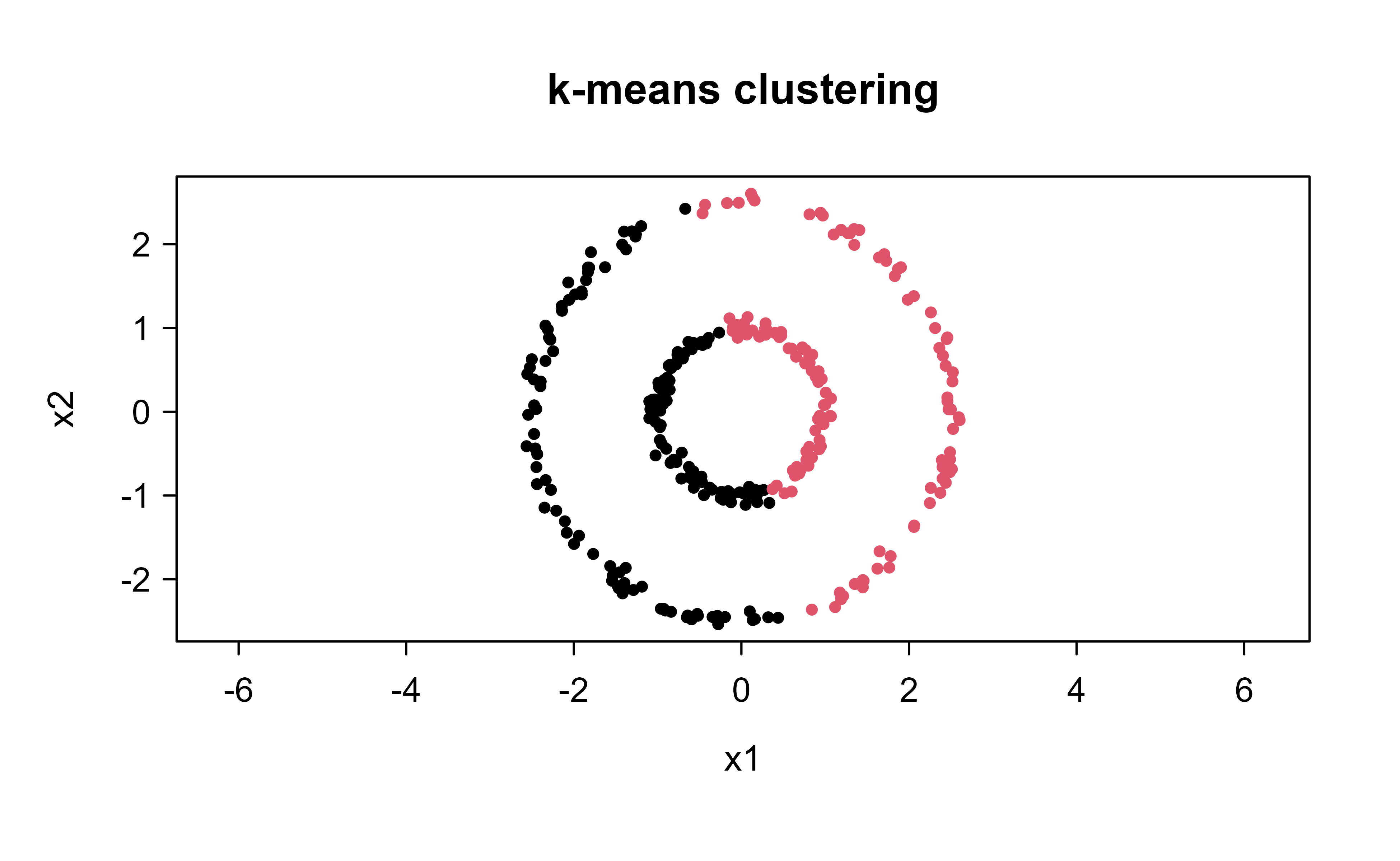
First, plain k-means with two centers. Figure 25.1 shows it slicing the rings down the middle rather than separating inner from outer, because no two centroids can wrap around a ring.
Show code
km<-kmeans(X, centers =2, nstart =20)plot(X, col =km$cluster, pch =19, cex =0.6, xlab ="x1", ylab ="x2", asp =1, main ="k-means clustering")
Figure 25.1: K-means on two concentric rings. The two centroids split the plane with a straight boundary, cutting each ring in half instead of separating the inner ring from the outer ring.
Now the spectral algorithm. We build a Gaussian affinity graph, form the symmetric normalized Laplacian, take its two smallest eigenvectors, row-normalize, and run k-means on the rows.
Show code
# 1. Gaussian similarity graph (fully connected, local bandwidth)D2<-as.matrix(dist(X))^2sigma<-0.3W<-exp(-D2/(2*sigma^2))diag(W)<-0# 2. Symmetric normalized Laplacian L_sym = I - D^{-1/2} W D^{-1/2}deg<-rowSums(W)Dm12<-diag(1/sqrt(deg))Lsym<-diag(n)-Dm12%*%W%*%Dm12# 3. k smallest eigenvectorsk<-2eig<-eigen(Lsym, symmetric =TRUE)idx<-order(eig$values)[1:k]U<-eig$vectors[, idx, drop =FALSE]# 4. row-normalize (Ng-Jordan-Weiss)Tmat<-U/sqrt(rowSums(U^2))# 5. k-means on the embedded rowssc<-kmeans(Tmat, centers =k, nstart =20)
The eigenvalues confirm the structure: the two smallest are essentially zero and there is a clear gap before the rest, the eigengap signal for two well-separated groups.
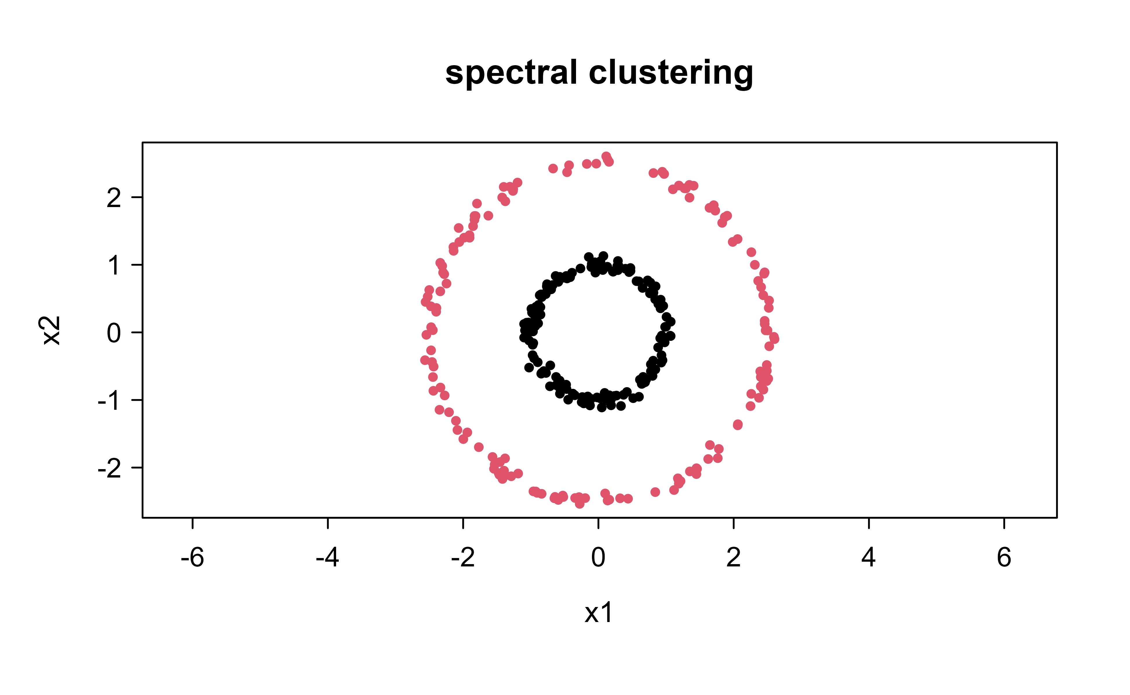
Figure 25.2 shows the spectral labels mapped back onto the original points. Inner and outer rings are now cleanly separated, the grouping k-means could not produce.
Show code
plot(X, col =sc$cluster, pch =19, cex =0.6, xlab ="x1", ylab ="x2", asp =1, main ="spectral clustering")
Figure 25.2: Spectral clustering of the same two rings. Clustering the graph Laplacian eigenvectors recovers the inner and outer rings exactly, the non-convex grouping that defeats k-means.
Finally we quantify the difference. We report clustering accuracy against the known ring labels, taking the better of the two label matchings since cluster numbering is arbitrary.
K-means lands near \(0.5\), no better than chance on this geometry, while spectral clustering recovers the rings essentially perfectly. The lesson generalizes: whenever the meaningful groups are connected but not convex, moving from raw coordinates to a graph-Laplacian embedding turns an impossible k-means problem into an easy one.
Tip
For real work, prefer the kernlab package (specc) or Spectrum, which handle sparse \(k\)NN graphs, eigengap-based selection of \(k\), and automatic bandwidth tuning. The hand-rolled code above is for understanding the mechanics, not for production at scale.
25.7 Summary
Spectral clustering reframes clustering as a graph-partitioning problem and solves a continuous relaxation of it. Build a similarity graph, form a graph Laplacian, and the balanced-cut objective (RatioCut or Ncut) relaxes through the Rayleigh quotient to an eigenvector problem in which the constant first eigenvector is trivial and the informative split lives in the second and subsequent eigenvectors. Embedding the points by the \(k\) smallest eigenvectors and running k-means on the rows then recovers groups, including the non-convex shapes such as concentric rings that k-means (Chapter 23) cannot find. The eigenvector embedding is a nonlinear dimension reduction (Chapter 27) closely tied to the spectral graph theory behind graph neural networks (Chapter 44). The price is an \(O(n^3)\) eigendecomposition and sensitivity to the graph construction, both managed in practice with sparse graphs, iterative eigensolvers, and the Nystrom approximation.
Source Code
# Spectral Clustering {#sec-spectral-clustering}```{r}#| include: falsesource("_common.R")```K-means (@sec-cluster) carves space into convex pieces. It asks, for each point, which centroid is nearest, and a region of points closer to one center than to all others is always convex. That works beautifully when the groups really are compact blobs, and it fails just as reliably when they are not. Picture two thin rings, one nested inside the other, like a dartboard. Every human sees two groups instantly. K-means sees one cloud of points and slices it down the middle, splitting each ring in half, because no placement of two centroids can wrap a center around a ring.Spectral clustering solves exactly this problem, and it does so with a change of viewpoint that is worth stating up front. Instead of trusting raw geometric distance, we build a graph: each observation is a node, and we connect nodes that are close, weighting the connection by how close they are. Two points on the same ring are linked through a long chain of near neighbors, even though the ends of the chain are far apart in Euclidean terms. Clustering then becomes a question about the graph, namely how to cut it into pieces while severing as few (and as weak) connections as possible. The surprising and beautiful fact is that the best such cut is encoded in the eigenvectors of a matrix attached to the graph, the graph Laplacian. Computing a few eigenvectors and running ordinary k-means on them recovers groups that raw k-means could never find.This chapter develops that story in full. We construct the similarity graph, define the unnormalized and normalized graph Laplacians and prove their core properties, derive how the combinatorial cut objective relaxes to an eigenvector problem (this is where the Rayleigh quotient and the "second eigenvector" enter), state the complete algorithm, explain when and why it beats k-means, and close with a runnable base-R demonstration on two concentric rings. Spectral clustering sits at the intersection of clustering (@sec-cluster), dimension reduction (@sec-dimension-reduction), since the eigenvectors are a nonlinear embedding, and the spectral graph theory that also underlies graph neural networks (@sec-graph-neural-networks).::: {.callout-important title="Key idea"}Spectral clustering does not cluster the data points. It clusters a low-dimensional embedding of the points built from the eigenvectors of a graph Laplacian. The hard, non-convex grouping problem in the original space becomes an easy, convex one in the embedded space, where plain k-means suffices.:::## The Similarity GraphThe first ingredient is a way to say which observations are "connected" and how strongly. Given data points $x_1, \dots, x_n$, we form a weighted undirected graph $G = (V, E)$ with one vertex per point. The edge weights are collected in a symmetric similarity (or affinity) matrix $W \in \mathbb{R}^{n \times n}$, where $w_{ij} \ge 0$ measures how similar points $i$ and $j$ are, with $w_{ij} = 0$ meaning no edge. Symmetry $w_{ij} = w_{ji}$ makes the graph undirected. Note the reversal relative to @sec-cluster, where we worked with a dissimilarity matrix $\mathbf{D}$ that is *small* for similar points; here $W$ is *large* for similar points.The standard recipe turns distances into similarities through a Gaussian (radial) kernel,$$w_{ij} = \exp\!\left( -\frac{\lVert x_i - x_j \rVert^2}{2 \sigma^2} \right),$$ {#eq-spectral-clustering-gaussian-affinity}with $w_{ii}$ usually set to $0$ so a point is not its own neighbor. The bandwidth $\sigma$ controls locality: small $\sigma$ keeps only very near points connected, large $\sigma$ links everything. This is the same kernel that appears in kernel smoothing (@sec-kernel) and Gaussian process regression (@sec-gaussian-process-reg), and the connection is not a coincidence, since spectral clustering can be read as kernel k-means.In practice one rarely uses the full dense $W$. Three standard sparsifications keep only local structure, which is both cheaper and more faithful to the manifold the data lie on.- The $\varepsilon$-neighborhood graph connects $i$ and $j$ if $\lVert x_i - x_j \rVert \le \varepsilon$. Because all kept edges have roughly equal length, edges are often left unweighted.- The $k$-nearest-neighbor graph connects $i$ to $j$ if $j$ is among the $k$ nearest neighbors of $i$. This relation is not symmetric, so one symmetrizes, either by connecting if *either* is a neighbor of the other (the usual choice) or only if *both* are (the mutual $k$NN graph).- The fully connected graph keeps every edge with weight from @eq-spectral-clustering-gaussian-affinity. This is sensible only with a local kernel like the Gaussian, whose weights decay fast.::: {.callout-warning}The result of spectral clustering can change substantially with the graph construction and the scale parameter ($\sigma$ or $k$ or $\varepsilon$). There is no single correct choice. Treat graph construction as a modeling decision, inspect the resulting graph for isolated points or accidental bridges between groups, and check that conclusions are stable across a range of scales.:::## Graph LaplaciansThe central object is the graph Laplacian. Define the degree of vertex $i$ as the total weight of edges touching it,$$d_i = \sum_{j=1}^n w_{ij},$$ {#eq-spectral-clustering-degree}and let $D = \operatorname{diag}(d_1, \dots, d_n)$ be the diagonal degree matrix. The unnormalized graph Laplacian is$$L = D - W.$$ {#eq-spectral-clustering-unnorm-laplacian}Two normalized variants matter in practice, the symmetric Laplacian and the random-walk Laplacian,$$L_{\mathrm{sym}} = D^{-1/2} L\, D^{-1/2} = I - D^{-1/2} W D^{-1/2},\qquadL_{\mathrm{rw}} = D^{-1} L = I - D^{-1} W .$$ {#eq-spectral-clustering-norm-laplacians}The name $L_{\mathrm{rw}}$ comes from the random walk on the graph whose transition matrix is $P = D^{-1} W$; then $L_{\mathrm{rw}} = I - P$, and clustering by $L_{\mathrm{rw}}$ amounts to finding sets the random walk seldom leaves.The single most important property of $L$ is the quadratic-form identity, which says $L$ measures how much a function varies across edges.::: {.callout-note title="The Laplacian quadratic form"}For any vector $f \in \mathbb{R}^n$,$$f^\top L f = \frac{1}{2} \sum_{i=1}^n \sum_{j=1}^n w_{ij}\, (f_i - f_j)^2 .$$ {#eq-spectral-clustering-quadratic-form}:::To see @eq-spectral-clustering-quadratic-form, expand using $d_i = \sum_j w_{ij}$,$$\begin{aligned}f^\top L f&= f^\top D f - f^\top W f = \sum_i d_i f_i^2 - \sum_{i,j} w_{ij} f_i f_j \\&= \frac{1}{2}\Big( \sum_i d_i f_i^2 - 2\sum_{i,j} w_{ij} f_i f_j + \sum_j d_j f_j^2 \Big) \\&= \frac{1}{2} \sum_{i,j} w_{ij}\, (f_i - f_j)^2 .\end{aligned}$$ {#eq-spectral-clustering-quadratic-derivation}The middle step rewrites $\sum_i d_i f_i^2 = \tfrac12(\sum_i d_i f_i^2 + \sum_j d_j f_j^2)$ and uses $d_i = \sum_j w_{ij}$ to turn each degree term into a double sum. Three consequences follow at once.1. Because every $w_{ij} \ge 0$, @eq-spectral-clustering-quadratic-form gives $f^\top L f \ge 0$, so $L$ is symmetric positive semidefinite. Its eigenvalues are real and nonnegative, $0 = \lambda_1 \le \lambda_2 \le \cdots \le \lambda_n$.2. The constant vector $\mathbf{1} = (1, \dots, 1)^\top$ satisfies $L\mathbf{1} = 0$ since each row of $L$ sums to zero, so $\lambda_1 = 0$ with eigenvector $\mathbf{1}$.3. The multiplicity of the eigenvalue $0$ equals the number of connected components of the graph, and the corresponding eigenspace is spanned by the indicator vectors of those components.Property 3 is the cleanest way to understand why spectral clustering works, so it is worth proving.::: {.callout-note title="Eigenvalue 0 counts connected components"}Let the graph have connected components $A_1, \dots, A_m$. Then the eigenvalue $0$ of $L$ has multiplicity $m$, and its eigenspace is spanned by the indicator vectors $\mathbf{1}_{A_1}, \dots, \mathbf{1}_{A_m}$, where $(\mathbf{1}_{A})_i = 1$ if $i \in A$ and $0$ otherwise.:::For the proof, suppose $Lf = 0$. Then $0 = f^\top L f = \tfrac12 \sum_{i,j} w_{ij}(f_i - f_j)^2$ by @eq-spectral-clustering-quadratic-form. Every term is nonnegative, so each must vanish: whenever $w_{ij} > 0$ we need $f_i = f_j$. Hence $f$ is constant on each connected component (within a component any two vertices are joined by a path of positive-weight edges, forcing equality along the path). So every null vector is a linear combination of the component indicators, and conversely each $\mathbf{1}_{A_\ell}$ is clearly in the null space. The indicators are linearly independent (disjoint supports), giving null-space dimension exactly $m$.This is the ideal case. If the data formed $k$ perfectly separated groups, the $k$ smallest eigenvectors of $L$ would be (rotations of) the cluster indicators, and reading off the clusters would be trivial. Real graphs are connected, so $\lambda_1 = 0$ is simple, but if the data have $k$ well-separated groups joined by only weak edges, the next $k-1$ eigenvalues stay near $0$ and their eigenvectors are nearly piecewise constant on the groups. This near-ideal structure is what k-means on the eigenvectors then recovers, and matrix perturbation theory (the Davis-Kahan theorem) makes the "nearly" precise.## From Graph Cuts to EigenvectorsWe now derive the algorithm by writing clustering as a graph-cut problem and relaxing it. For two disjoint vertex sets $A, B$, define the cut as the total weight of severed edges,$$\operatorname{cut}(A, B) = \sum_{i \in A,\, j \in B} w_{ij} .$$ {#eq-spectral-clustering-cut}A natural objective for splitting the graph into $k$ parts $A_1, \dots, A_k$ is the total weight removed, $\sum_{\ell} \operatorname{cut}(A_\ell, \overline{A_\ell})$. Minimizing this raw cut, though, is a trap: it tends to lop off a single isolated vertex, because cutting off one weakly connected point removes very little weight. We need to insist that the pieces be substantial. The two standard fixes normalize the cut by the size of each part, measured either by the number of vertices $|A|$ or by the volume $\operatorname{vol}(A) = \sum_{i \in A} d_i$,$$\operatorname{RatioCut}(A_1, \dots, A_k) = \sum_{\ell=1}^k \frac{\operatorname{cut}(A_\ell, \overline{A_\ell})}{|A_\ell|},\qquad\operatorname{Ncut}(A_1, \dots, A_k) = \sum_{\ell=1}^k \frac{\operatorname{cut}(A_\ell, \overline{A_\ell})}{\operatorname{vol}(A_\ell)} .$$ {#eq-spectral-clustering-ncut-ratiocut}RatioCut balances by vertex count and leads to the unnormalized $L$; Ncut balances by volume and leads to $L_{\mathrm{rw}}$ and $L_{\mathrm{sym}}$. Both are NP-hard to minimize exactly, since each is a combinatorial optimization over all partitions. Spectral clustering is the continuous relaxation of these problems, and the relaxation is what produces an eigenvector computation.### The two-cluster relaxationTake $k = 2$ and RatioCut, which is the cleanest case and the one where the "second eigenvector" appears explicitly. We want to split $V$ into $A$ and $\overline{A}$. Encode the partition in a single vector $f \in \mathbb{R}^n$ with the clever values$$f_i =\begin{cases}\ \ \sqrt{\,|\overline{A}| / |A|\,}, & i \in A, \\[4pt]-\sqrt{\,|A| / |\overline{A}|\,}, & i \in \overline{A}.\end{cases}$$ {#eq-spectral-clustering-indicator}These specific magnitudes look arbitrary but are engineered so that three things hold simultaneously. First, plug $f$ into the Laplacian quadratic form. Only edges crossing between $A$ and $\overline{A}$ contribute (within a side $f_i - f_j = 0$), and each crossing edge contributes $(f_i - f_j)^2 = \big(\sqrt{|\overline A|/|A|} + \sqrt{|A|/|\overline A|}\big)^2$. A short simplification of that square gives$$\begin{aligned}f^\top L f&= \tfrac12 \sum_{i,j} w_{ij}(f_i - f_j)^2 = \operatorname{cut}(A, \overline{A})\left( \frac{|\overline{A}|}{|A|} + \frac{|A|}{|\overline{A}|} + 2 \right) \\&= \operatorname{cut}(A, \overline{A})\, \frac{(|A| + |\overline{A}|)^2}{|A|\,|\overline{A}|} = n\left( \frac{\operatorname{cut}(A,\overline A)}{|A|} + \frac{\operatorname{cut}(A,\overline A)}{|\overline A|} \right) = n \cdot \operatorname{RatioCut}(A, \overline{A}),\end{aligned}$$ {#eq-spectral-clustering-ratiocut-objective}using $|A| + |\overline A| = n$. So minimizing RatioCut is exactly minimizing $f^\top L f$ over vectors $f$ of the form @eq-spectral-clustering-indicator. Second, this encoding makes $f$ orthogonal to the constant vector,$$\sum_i f_i = |A|\sqrt{\tfrac{|\overline A|}{|A|}} - |\overline A|\sqrt{\tfrac{|A|}{|\overline A|}} = \sqrt{|A|\,|\overline A|} - \sqrt{|A|\,|\overline A|} = 0,$$ {#eq-spectral-clustering-orthogonality}that is $f \perp \mathbf{1}$. Third, the encoding fixes the scale, $\lVert f \rVert^2 = \sum_i f_i^2 = |A|\frac{|\overline A|}{|A|} + |\overline A|\frac{|A|}{|\overline A|} = n$, so $\lVert f \rVert = \sqrt{n}$.Collecting these, exact RatioCut minimization is$$\min_{A}\ f^\top L f\quad \text{subject to} \quadf \perp \mathbf{1},\quad \lVert f \rVert = \sqrt{n},$$ {#eq-spectral-clustering-discrete-problem}with $f$ further restricted to the two-valued form of @eq-spectral-clustering-indicator. That discreteness, the requirement that $f$ take only the two special values, is what makes this NP-hard. The relaxation simply drops that last constraint and lets $f$ range over all real vectors,$$\min_{f \in \mathbb{R}^n}\ f^\top L f\quad \text{subject to} \quadf \perp \mathbf{1},\quad \lVert f \rVert = \sqrt{n}.$$ {#eq-spectral-clustering-relaxed-problem}### Why the second eigenvectorProblem @eq-spectral-clustering-relaxed-problem is a Rayleigh-quotient minimization. The Rayleigh quotient of a symmetric matrix $L$ is $R(f) = \dfrac{f^\top L f}{f^\top f}$, and the Courant-Fischer theorem says its constrained minima are the eigenvectors of $L$. Concretely, the unconstrained minimizer of $R$ is the eigenvector of the smallest eigenvalue, which here is $\mathbf{1}$ with eigenvalue $0$. But we have explicitly forbidden $f \propto \mathbf{1}$ via the constraint $f \perp \mathbf{1}$. Minimizing the Rayleigh quotient over the subspace orthogonal to the first eigenvector yields the second eigenvector, the one belonging to the second-smallest eigenvalue $\lambda_2$.To see this with a Lagrange multiplier, minimize $f^\top L f$ subject to $\lVert f \rVert^2 = n$ (and $f \perp \mathbf 1$). The stationarity condition of $f^\top L f - \mu(f^\top f - n)$ is$$2 L f - 2 \mu f = 0 \quad\Longrightarrow\quad L f = \mu f,$$ {#eq-spectral-clustering-lagrange}so any solution is an eigenvector of $L$, and at such an $f$ the objective equals $f^\top L f = \mu \lVert f\rVert^2 = \mu n$. To make the objective small we want the smallest eigenvalue $\mu$, but the constraint $f \perp \mathbf 1$ rules out $\mu = \lambda_1 = 0$. The smallest admissible choice is $\mu = \lambda_2$, with $f$ the second eigenvector $u_2$, the so-called Fiedler vector. This is the precise sense in which "the second eigenvector matters": the first eigenvector is the trivial constant that the balancing constraint removes, and the first *informative* direction, the one that splits the graph, is the second.We then recover a discrete partition by thresholding $u_2$, for example assigning $i \in A$ when $u_{2,i} \ge 0$ and $i \in \overline A$ otherwise. The same derivation with the volume-weighted indicator and the generalized eigenproblem $L u = \lambda D u$ (equivalently the eigenvectors of $L_{\mathrm{rw}}$) yields Ncut instead of RatioCut.::: {.callout-tip}The relaxation is genuinely a relaxation, so the cut it returns is not guaranteed to equal the true optimum. There exist constructed graphs where the gap is large. In practice the relaxation is excellent precisely when the clusters are well separated, which is the regime where we want clustering to work anyway.:::### From two clusters to $k$For general $k$ we use the $k$ smallest eigenvectors at once. Stack $u_1, \dots, u_k$ as columns of $U \in \mathbb{R}^{n \times k}$. The relaxed multiway RatioCut problem is the trace minimization$$\min_{U \in \mathbb{R}^{n \times k}}\ \operatorname{tr}(U^\top L\, U)\quad \text{subject to} \quad U^\top U = I_k,$$ {#eq-spectral-clustering-trace-min}whose solution (again by Courant-Fischer, in its trace form) is the matrix of the $k$ eigenvectors with smallest eigenvalues, unique up to rotation. Each row of $U$ is the embedding of one data point into $\mathbb{R}^k$. In the ideal disconnected case those rows collapse to $k$ distinct points (the indicator structure of the previous section), so running k-means on the rows is the natural way to convert the relaxed, continuous embedding back into a hard clustering.## The AlgorithmThe pieces assemble into the normalized spectral clustering of Ng, Jordan, and Weiss, which uses $L_{\mathrm{sym}}$ and an extra row-normalization step.1. Build the similarity matrix $W$ from the data via @eq-spectral-clustering-gaussian-affinity (with an $\varepsilon$-, $k$NN, or full graph), and set $\operatorname{diag}(W) = 0$.2. Compute degrees $d_i = \sum_j w_{ij}$, form $D$, and the Laplacian. For the normalized version, $L_{\mathrm{sym}} = I - D^{-1/2} W D^{-1/2}$.3. Compute the $k$ eigenvectors $u_1, \dots, u_k$ of $L_{\mathrm{sym}}$ with the $k$ smallest eigenvalues, and stack them as columns of $U \in \mathbb{R}^{n \times k}$.4. Form $T$ by normalizing each row of $U$ to unit length, $T_{ij} = U_{ij} / (\sum_\ell U_{i\ell}^2)^{1/2}$. (This row-normalization is what distinguishes $L_{\mathrm{sym}}$ from $L_{\mathrm{rw}}$; it undoes the degree scaling that $D^{-1/2}$ introduced into the eigenvectors.)5. Treat each row of $T$ as a point in $\mathbb{R}^k$ and cluster the rows with k-means into $k$ groups.6. Assign original point $i$ to the cluster that received row $i$.Choosing $k$ uses the eigengap heuristic: order the eigenvalues $\lambda_1 \le \lambda_2 \le \cdots$ and pick $k$ so that $\lambda_1, \dots, \lambda_k$ are small while $\lambda_{k+1}$ is comparatively large. A large gap after the $k$-th eigenvalue signals $k$ well-separated groups, mirroring the exact "multiplicity equals number of components" result.::: {.callout-note title="Complexity"}Forming a dense $W$ and the eigendecomposition cost $O(n^2)$ memory and up to $O(n^3)$ time, so naive spectral clustering does not scale to very large $n$. The standard remedies are a sparse $k$NN graph (so $W$ has $O(nk)$ nonzeros), a Lanczos-type iterative solver that returns only the few smallest eigenvectors at roughly $O(\text{nnz} \cdot k)$ per iteration, and the Nystrom method, which approximates the eigenvectors from a sampled subset of columns. These bring spectral clustering within reach of large datasets at the cost of approximation.:::## When It Beats K-Means, and When It Does NotSpectral clustering's advantage is its ability to find non-convex, non-spherical clusters that k-means cannot. K-means assigns by Euclidean distance to a centroid, so its clusters are always convex blobs of comparable spread. Two interlocking moons, two concentric rings, or a small ball nested inside a large shell all defeat it. Spectral clustering escapes this because it never compares points by raw distance once the graph is built; it compares them by connectivity through the graph, and connectivity follows the shape of the data manifold rather than straight-line geometry. The eigenvector embedding then maps each connected, manifold-shaped group to a tight blob, exactly the situation k-means handles well, which is why k-means is run on the embedding rather than on the original data. This is closely related to using the embedding as a nonlinear feature map, the same spirit as kernel methods and the spectral view of graph neural networks (@sec-graph-neural-networks).The cost of this power is sensitivity and expense. Results depend on the graph and on the scale parameter $\sigma$, an unlucky bandwidth bridges two groups or fragments one. The $O(n^3)$ eigendecomposition is far heavier than the $O(nKpI)$ of k-means. There is no centroid to assign new out-of-sample points, so labeling fresh data requires re-running or an explicit out-of-sample extension. And the method still needs $k$ specified, though the eigengap offers more guidance than k-means usually has. A reasonable rule of thumb: reach for k-means or a Gaussian mixture when groups are roughly elliptical blobs, and reach for spectral clustering when you have reason to expect connected but curved or interlocking structure, or when a meaningful similarity graph is more natural than a coordinate representation.## A Runnable Demonstration: Two Concentric RingsWe now make the headline example concrete. We generate two concentric rings, the case where k-means provably fails, and show that the spectral algorithm recovers them exactly. The code uses only base R (`dist`, `eigen`, `kmeans`).```{r}#| label: spectral-rings-setupset.seed(1)# Two concentric rings: inner radius 1, outer radius 2.5make_ring <-function(n, r, noise) { theta <-runif(n, 0, 2* pi) rad <- r +rnorm(n, 0, noise)cbind(rad *cos(theta), rad *sin(theta))}n_per <-150X <-rbind(make_ring(n_per, 1.0, 0.06),make_ring(n_per, 2.5, 0.06))truth <-rep(c(1, 2), each = n_per)n <-nrow(X)```First, plain k-means with two centers. @fig-spectral-clustering-kmeans shows it slicing the rings down the middle rather than separating inner from outer, because no two centroids can wrap around a ring.```{r}#| label: fig-spectral-clustering-kmeans#| fig-cap: "K-means on two concentric rings. The two centroids split the plane with a straight boundary, cutting each ring in half instead of separating the inner ring from the outer ring."km <-kmeans(X, centers =2, nstart =20)plot(X, col = km$cluster, pch =19, cex =0.6,xlab ="x1", ylab ="x2", asp =1,main ="k-means clustering")```Now the spectral algorithm. We build a Gaussian affinity graph, form the symmetric normalized Laplacian, take its two smallest eigenvectors, row-normalize, and run k-means on the rows.```{r}#| label: spectral-rings-fit# 1. Gaussian similarity graph (fully connected, local bandwidth)D2 <-as.matrix(dist(X))^2sigma <-0.3W <-exp(-D2 / (2* sigma^2))diag(W) <-0# 2. Symmetric normalized Laplacian L_sym = I - D^{-1/2} W D^{-1/2}deg <-rowSums(W)Dm12 <-diag(1/sqrt(deg))Lsym <-diag(n) - Dm12 %*% W %*% Dm12# 3. k smallest eigenvectorsk <-2eig <-eigen(Lsym, symmetric =TRUE)idx <-order(eig$values)[1:k]U <- eig$vectors[, idx, drop =FALSE]# 4. row-normalize (Ng-Jordan-Weiss)Tmat <- U /sqrt(rowSums(U^2))# 5. k-means on the embedded rowssc <-kmeans(Tmat, centers = k, nstart =20)```The eigenvalues confirm the structure: the two smallest are essentially zero and there is a clear gap before the rest, the eigengap signal for two well-separated groups.```{r}#| label: spectral-rings-eigvalsround(sort(eig$values)[1:6], 4)```@fig-spectral-clustering-result shows the spectral labels mapped back onto the original points. Inner and outer rings are now cleanly separated, the grouping k-means could not produce.```{r}#| label: fig-spectral-clustering-result#| fig-cap: "Spectral clustering of the same two rings. Clustering the graph Laplacian eigenvectors recovers the inner and outer rings exactly, the non-convex grouping that defeats k-means."plot(X, col = sc$cluster, pch =19, cex =0.6,xlab ="x1", ylab ="x2", asp =1,main ="spectral clustering")```Finally we quantify the difference. We report clustering accuracy against the known ring labels, taking the better of the two label matchings since cluster numbering is arbitrary.```{r}#| label: spectral-rings-accuracyagree <-function(a, b) max(mean(a == b), mean(a == (3- b)))c(kmeans =round(agree(km$cluster, truth), 3),spectral =round(agree(sc$cluster, truth), 3))```K-means lands near $0.5$, no better than chance on this geometry, while spectral clustering recovers the rings essentially perfectly. The lesson generalizes: whenever the meaningful groups are connected but not convex, moving from raw coordinates to a graph-Laplacian embedding turns an impossible k-means problem into an easy one.::: {.callout-tip}For real work, prefer the `kernlab` package (`specc`) or `Spectrum`, which handle sparse $k$NN graphs, eigengap-based selection of $k$, and automatic bandwidth tuning. The hand-rolled code above is for understanding the mechanics, not for production at scale.:::## SummarySpectral clustering reframes clustering as a graph-partitioning problem and solves a continuous relaxation of it. Build a similarity graph, form a graph Laplacian, and the balanced-cut objective (RatioCut or Ncut) relaxes through the Rayleigh quotient to an eigenvector problem in which the constant first eigenvector is trivial and the informative split lives in the second and subsequent eigenvectors. Embedding the points by the $k$ smallest eigenvectors and running k-means on the rows then recovers groups, including the non-convex shapes such as concentric rings that k-means (@sec-cluster) cannot find. The eigenvector embedding is a nonlinear dimension reduction (@sec-dimension-reduction) closely tied to the spectral graph theory behind graph neural networks (@sec-graph-neural-networks). The price is an $O(n^3)$ eigendecomposition and sensitivity to the graph construction, both managed in practice with sparse graphs, iterative eigensolvers, and the Nystrom approximation.