Most of the methods in this book assume that the rows of a data set are exchangeable: we could shuffle them without losing anything, and a random train/test split is a fair test of generalization. Time series break that assumption. A measurement at noon is not interchangeable with a measurement at midnight, last month’s value tells you a great deal about this month’s, and the future is, by definition, the part of the data you have not seen yet. Forecasting is the task of using the ordered past to say something useful about the ordered future.
This chapter builds the topic from the ground up. We start with the forecasting setup and the notation, explain why naive cross-validation leaks information across time, and then construct the two ingredients that make modern machine-learning forecasters work: lag features and rolling-window summaries. With those in hand we compare three families of forecasters on a real series: classical statistical baselines (the naive forecast, exponential smoothing, and ARIMA), tree-based machine learning (gradient boosting, Chapter 12), and a brief look at deep sequence models. Throughout, the running example forecasts monthly airline passenger counts, and every claim about accuracy is backed by a rolling-origin evaluation rather than a single lucky split.
Intuition
A forecaster is a function that maps “everything known up to now” into “a guess about what comes next.” The art is choosing what to feed it (features) and how to score it honestly (evaluation that respects time).
88.1 The Forecasting Setup
Let \(\{y_t\}_{t=1}^{T}\) be a univariate time series observed at regular intervals, where \(t\) indexes time and \(y_t \in \mathbb{R}\) is the value at time \(t\). We may also observe exogenous predictors \(\mathbf{x}_t \in \mathbb{R}^{p}\) (for example a holiday flag or a promotion indicator). The information set available at time \(t\) is
\[
\mathcal{F}_t = \{\, y_s, \mathbf{x}_s : s \le t \,\},
\]
the entire ordered history through time \(t\). A point forecast made at the forecast origin \(t\) for a target \(h\) steps ahead is written
read as “the prediction of \(y_{t+h}\) given information through \(t\).” The integer \(h \ge 1\) is the forecast horizon. Forecasting one step ahead (\(h=1\)) is the easiest case; multi-step forecasting (\(h > 1\)) is harder because errors accumulate and because the inputs you would like to use (recent values of \(y\)) are themselves unknown for the steps in between.
The quantity we ultimately care about is the forecast error,
\[
e_{t+h} = y_{t+h} - \hat{y}_{t+h\mid t},
\]
and a forecasting model is good if these errors are small and unbiased across many origins.
Key idea
Two numbers define every forecasting problem before you write any code: the horizon \(h\) (how far ahead) and the origin (the last time point you are allowed to use). Fixing them up front prevents almost every subtle mistake that follows.
88.1.1 Decomposition and What Models Try to Capture
A classical way to reason about a series is to imagine it as the sum of unobserved components,
\[
y_t = T_t + S_t + R_t,
\]
where \(T_t\) is a slowly varying trend, \(S_t\) is a seasonal pattern that repeats with known period \(m\) (for monthly data with yearly seasonality, \(m=12\)), and \(R_t\) is the remainder (the irregular part). When seasonal swings grow with the level of the series, a multiplicative form \(y_t = T_t \times S_t \times R_t\) fits better, and taking logs turns it back into an additive problem because \(\log y_t = \log T_t + \log S_t + \log R_t\). Every forecasting method in this chapter is, in effect, a different bet about how trend, seasonality, and noise combine.
88.2 Splitting Time Honestly: Backtesting and Leakage
The single most common error in applied forecasting is evaluating a model with a random split or with standard \(k\)-fold cross-validation. Both place future observations in the training set and past observations in the test set, which lets the model “peek” at information it would never have at deployment time. The result is an optimistic accuracy estimate that collapses in production.
Warning
Never shuffle a time series before splitting, and never use plain \(k\)-fold cross-validation on raw temporal data. Any procedure that lets a training point come from after a test point is leaking the future.
The honest alternative is rolling-origin evaluation, also called time-series cross-validation or backtesting. We pick an initial training window, forecast the next \(h\) steps, record the error, then move the origin forward and repeat. There are two common variants:
Expanding window: the training set grows as the origin advances (use all history up to the origin). Good when more history always helps.
Sliding window: the training set keeps a fixed length and drops the oldest points. Good when the data-generating process drifts and old data is misleading.
Formally, with origins \(t = t_0, t_0+1, \dots, T-h\), the rolling-origin estimate of a loss \(L\) at horizon \(h\) is the average over origins,
\[
\widehat{\text{CV}}_h = \frac{1}{N}\sum_{t=t_0}^{T-h} L\!\left(y_{t+h},\, \hat{y}_{t+h\mid t}\right),
\qquad N = T - h - t_0 + 1 .
\]
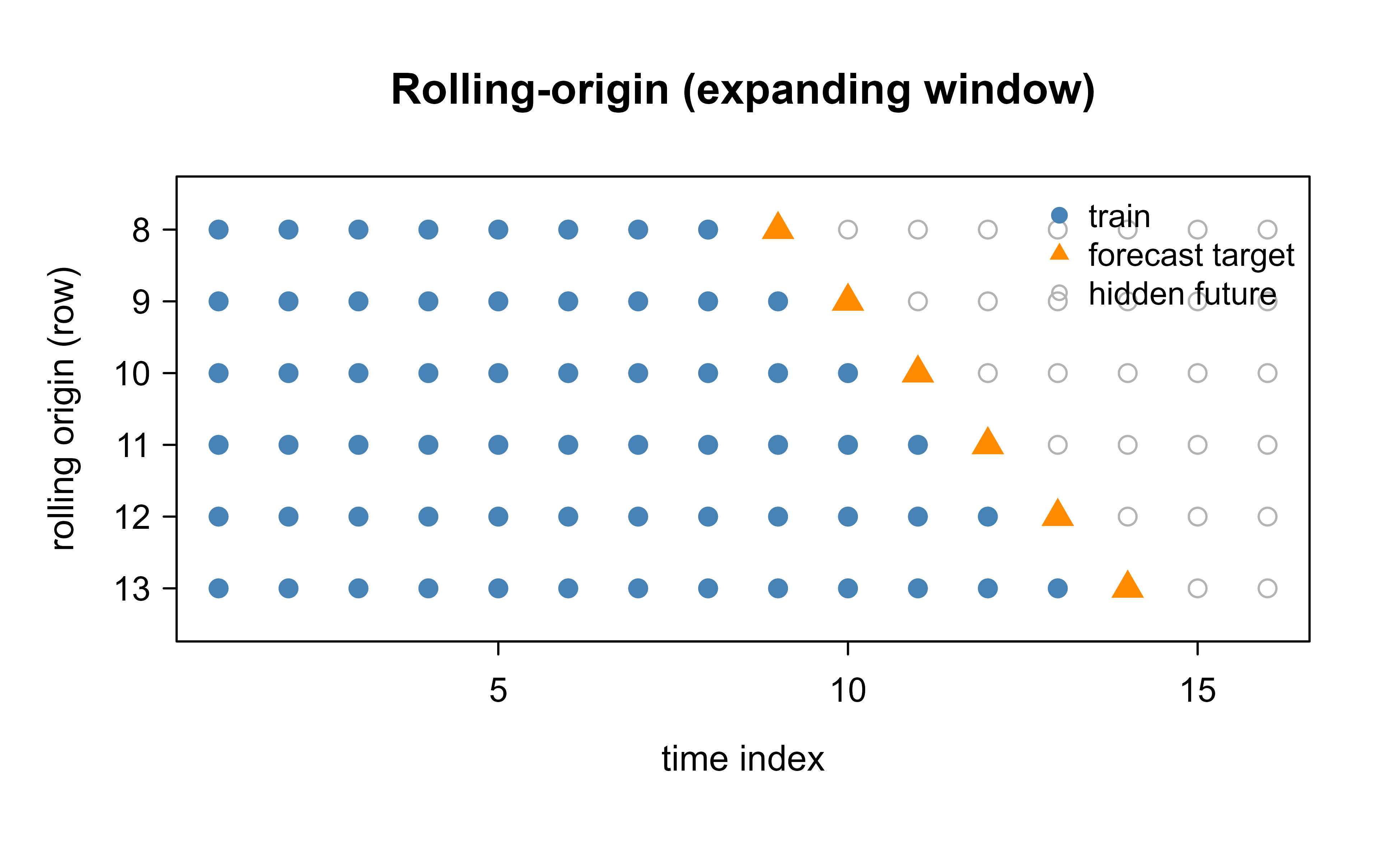
Figure 88.1 illustrates the expanding-window scheme: each row is one origin, blue points are training, the orange point is the value being forecast, and gray points are not yet visible to the model.
Show code
set.seed(1)n_pts<-16origins<-8:13plot(NA, xlim =c(1, n_pts), ylim =c(length(origins)+0.5, 0.5), xlab ="time index", ylab ="rolling origin (row)", yaxt ="n", main ="Rolling-origin (expanding window)")axis(2, at =seq_along(origins), labels =origins, las =1)for(rinseq_along(origins)){o<-origins[r]train<-1:otest<-o+1future<-if(test<n_pts)(test+1):n_ptselseinteger(0)points(train, rep(r, length(train)), pch =19, col ="steelblue", cex =1.1)points(test, r, pch =17, col ="darkorange", cex =1.5)if(length(future))points(future, rep(r, length(future)), pch =1, col ="gray70", cex =1.1)}legend("topright", legend =c("train", "forecast target", "hidden future"), pch =c(19, 17, 1), col =c("steelblue", "darkorange", "gray70"), bty ="n", cex =0.9)
Figure 88.1: Expanding-window rolling-origin evaluation. Each horizontal row is one forecast origin; the model trains on the blue points and is scored on the orange (future) point, while the gray points remain hidden. The origin advances downward, so no training point ever comes from after the point being scored.
Figure 88.1 makes the rule visual: read any row left to right and the orange target always sits to the right of every blue training point.
Note
Leakage also hides inside feature engineering. If you scale features using the mean and standard deviation of the whole series, or impute missing values with a global statistic, the training rows have absorbed information from the test period. Compute every such statistic on the training window only, inside each fold.
88.3 Turning a Time Series into a Supervised Learning Problem
Machine-learning regressors such as linear models, random forests, and gradient boosting do not know about time. They expect a feature matrix \(\mathbf{X}\) and a target vector \(\mathbf{y}\). The bridge from a series to that format is lag embedding: we define the target as the value \(h\) steps ahead and the features as a window of recent past values.
For one-step-ahead forecasting with \(k\) lags, the design is
so each training row is a length-\(k\) snapshot of history paired with the next value. This is exactly the autoregressive idea: the order-\(k\) autoregressive model \(\text{AR}(k)\) is the special case where \(f\) is linear,
\[
\hat{y}_{t} = c + \sum_{j=1}^{k}\phi_j\, y_{t-j}.
\]
Replacing that linear \(f\) with a tree ensemble or any other learner gives a nonlinear autoregression, which is the workhorse of machine-learning forecasting.
Two enrichments make lag features much stronger:
Rolling-window summaries. Beyond raw lags, summarize recent history with a moving statistic computed strictly from past values, for example a trailing mean over the last \(w\) points, \(\bar{y}_{t-1}^{(w)} = \frac{1}{w}\sum_{j=1}^{w} y_{t-j}\), or a trailing standard deviation. These smooth out noise and hand the model a ready-made notion of “recent level” and “recent volatility.”
Calendar features. Encode the position in the seasonal cycle (month of year, day of week) so the model can learn seasonality directly. For monthly data the month index \(1,\dots,12\) is enough for a tree; linear models prefer sine/cosine pairs such as \(\sin(2\pi m_t / 12)\) and \(\cos(2\pi m_t / 12)\).
Warning
Every feature must be computable at the forecast origin. A lag of order 1 uses \(y_{t-1}\), which is fine. A “centered” moving average that averages \(y_{t-1}, y_t, y_{t+1}\) is not: it uses the future. When in doubt, ask whether the feature could have been written down the moment before \(y_t\) was observed.
88.3.1 Multi-Step Horizons: Recursive vs Direct
Once we want \(h > 1\) steps, there are two standard strategies.
The recursive strategy trains a single one-step model and feeds its own predictions back as inputs: forecast \(\hat{y}_{t+1\mid t}\), then treat it as if observed to forecast \(\hat{y}_{t+2\mid t}\), and so on. It is simple and data-efficient but lets one-step errors compound across the horizon.
The direct strategy trains a separate model for each horizon, with target \(y_{t+h}\) regressed on features available at \(t\), for each \(h = 1, \dots, H\). It avoids error feedback at the cost of fitting \(H\) models and ignoring the relationship between consecutive horizons.
When to use this
Use the recursive strategy when you have little data or a short horizon, and the direct strategy when the horizon is long, you have enough data to fit several models, and you can tolerate the extra bookkeeping. Hybrid schemes exist, but starting with recursive and checking whether direct helps is a sound default.
88.4 A Worked Comparison on AirPassengers
We now forecast the built-in AirPassengers series: monthly totals of international airline passengers from 1949 to 1960, a classic example with a clear upward trend and strong yearly seasonality whose amplitude grows over time. We hold out the final 24 months as a test set, forecast them, and compare a naive seasonal baseline, exponential smoothing (ETS), ARIMA, and an xgboost regressor built on lag and calendar features.
The multiplicative seasonality (swings widen as the level rises) is exactly the case where a log transform helps, so the machine-learning model is trained on \(\log y_t\) and predictions are exponentiated back.
We construct lag features (orders 1, 2, 3, and the seasonal lag 12), trailing rolling summaries computed only from past values, and the month index. The helper below returns a data frame aligned so that row \(t\) holds the target \(y_t\) and features that were all knowable at time \(t-1\).
The first 12 rows have no seasonal lag and are dropped by complete.cases. This is normal: lag features always cost you a warm-up period equal to the largest lag.
88.4.2 Fitting the Models
We train ETS and ARIMA with the forecast package on the original scale (they handle the trend and seasonality internally), and an xgboost model on the engineered log-scale features. The seasonal naive forecast, which simply repeats the value from 12 months earlier, is our floor: any method that cannot beat it is not worth its complexity.
Show code
train_ts<-ts(y[train_idx], frequency =freq, start =c(1949, 1))# Classical baselinesfit_snaive<-snaive(train_ts, h =h_test)fit_ets<-forecast(ets(train_ts), h =h_test)fit_arima<-forecast(auto.arima(train_ts), h =h_test)# xgboost on engineered features (recursive multi-step below)tr<-sup_complete[sup_complete$row<=max(train_idx), ]dtrain<-xgb.DMatrix(as.matrix(tr[, feat_cols]), label =tr$target)set.seed(42)xgb_fit<-xgb.train( params =list(objective ="reg:squarederror", max_depth =3, eta =0.1, subsample =0.9, colsample_bytree =0.9), data =dtrain, nrounds =300, verbose =0)
The boosting model is one-step-ahead by construction, so to cover the 24-month horizon we forecast recursively: predict the next month, append the prediction to the history, recompute the lag and rolling features, and step forward.
Show code
recursive_forecast<-function(model, y_log_hist, month_future, h,lags=c(1, 2, 3, 12),roll_windows=c(3, 12), feat_cols){hist<-y_log_hist# log-scale history, grows as we predictpreds<-numeric(h)for(iinseq_len(h)){Ncur<-length(hist)row<-list(month =month_future[i])for(Linlags)row[[paste0("lag", L)]]<-hist[Ncur-L+1]for(winroll_windows){win<-hist[(Ncur-w+1):Ncur]row[[paste0("rollmean", w)]]<-mean(win)row[[paste0("rollsd", w)]]<-sd(win)}xrow<-as.matrix(as.data.frame(row)[, feat_cols, drop =FALSE])p<-predict(model, xgb.DMatrix(xrow))preds[i]<-phist<-c(hist, p)# feed prediction back}preds}month_future<-month_of_year[test_idx]xgb_log_pred<-recursive_forecast(xgb_fit, log(y[train_idx]), month_future, h_test, feat_cols =feat_cols)xgb_pred<-exp(xgb_log_pred)# back to passenger counts
88.4.3 Visualizing the Forecasts
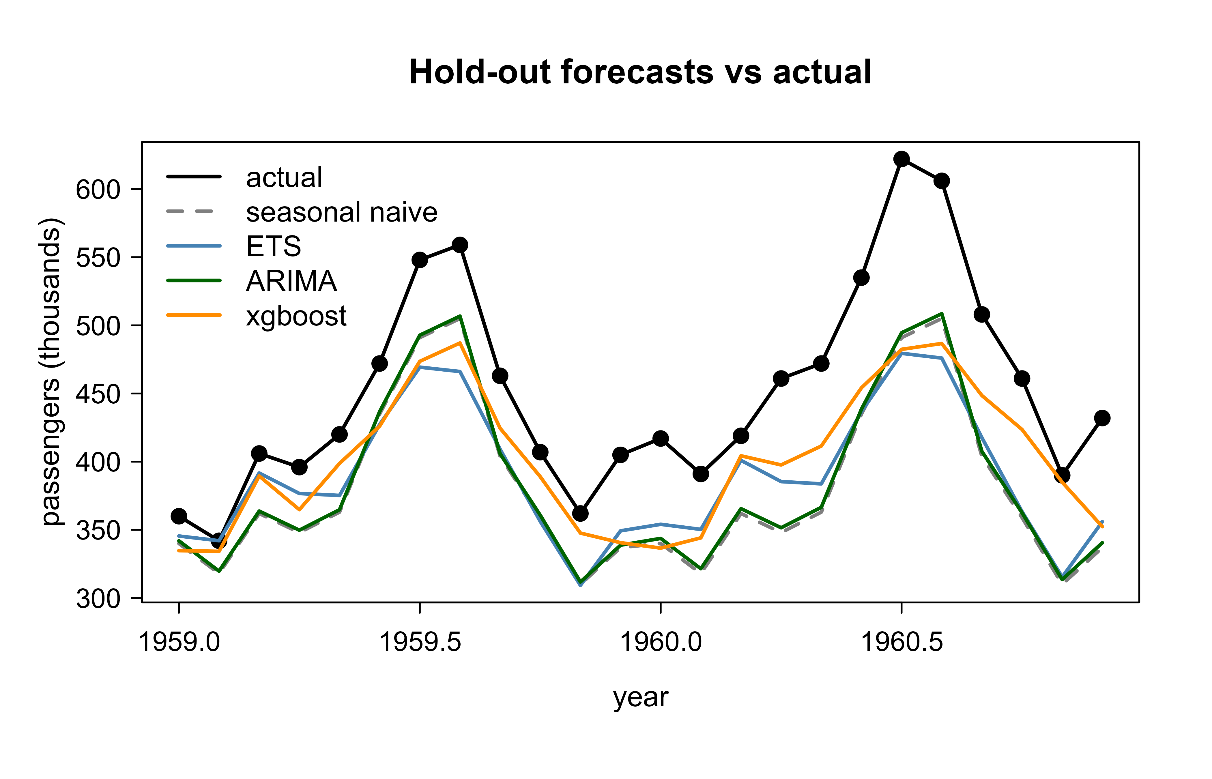
Figure 88.2 overlays the four forecasts on the held-out period. The seasonal naive forecast keeps the right shape but misses the growth; ETS and ARIMA track both trend and seasonality closely; the boosting model, trained only on lags and calendar position, recovers the seasonal pattern from data alone.
Show code
actual<-y[test_idx]time_test<-time(AirPassengers)[test_idx]plot(time_test, actual, type ="o", pch =19, lwd =2, ylim =range(actual, fit_ets$mean, fit_arima$mean, xgb_pred,fit_snaive$mean), xlab ="year", ylab ="passengers (thousands)", main ="Hold-out forecasts vs actual")lines(time_test, as.numeric(fit_snaive$mean), col ="gray50", lwd =2, lty =2)lines(time_test, as.numeric(fit_ets$mean), col ="steelblue", lwd =2)lines(time_test, as.numeric(fit_arima$mean), col ="darkgreen", lwd =2)lines(time_test, xgb_pred, col ="darkorange", lwd =2)legend("topleft", bty ="n", lwd =2, lty =c(1, 2, 1, 1, 1), col =c("black", "gray50", "steelblue", "darkgreen", "darkorange"), legend =c("actual", "seasonal naive", "ETS", "ARIMA", "xgboost"))
Figure 88.2: Forecasts of monthly AirPassengers counts over the 24-month hold-out period. The black line is the truth; colored lines are the seasonal naive, ETS, ARIMA, and xgboost forecasts. ETS, ARIMA, and xgboost all capture trend and seasonality, while the seasonal naive baseline misses the upward growth.
Figure 88.2 is a single-split snapshot. To judge the methods fairly we must average over many origins, which is the next step.
88.4.4 Rolling-Origin Evaluation
We score each method with an expanding-window backtest at horizon \(h=1\). Starting from an initial window of 100 months, we forecast the next month, advance the origin, and repeat to the end of the series. The error metrics are the mean absolute error (MAE) and the root mean squared error (RMSE),
and the mean absolute scaled error (MASE), which divides MAE by the in-sample MAE of the seasonal naive forecast so that a value below 1 means “better than the seasonal naive baseline.”
Show code
init<-100Lorigins<-init:(n-1L)# one-step-ahead originserr_snaive<-err_ets<-err_arima<-err_xgb<-numeric(length(origins))for(kinseq_along(origins)){o<-origins[k]ytr<-ts(y[1:o], frequency =freq, start =c(1949, 1))truth<-y[o+1]# Seasonal naive: value from 12 months earliersn<-y[o+1-freq]# ETS and ARIMA refit each origin (small series, fast)e1<-as.numeric(forecast(ets(ytr), h =1)$mean)a1<-as.numeric(forecast(auto.arima(ytr), h =1)$mean)# xgboost: rebuild supervised frame on log scale up to o, fit, predict 1 stepsup_o<-make_supervised(log(y[1:o]), month_of_year[1:o])sup_o<-sup_o[stats::complete.cases(sup_o), ]d_o<-xgb.DMatrix(as.matrix(sup_o[, feat_cols]), label =sup_o$target)set.seed(42)m_o<-xgb.train( params =list(objective ="reg:squarederror", max_depth =3, eta =0.1, subsample =0.9, colsample_bytree =0.9), data =d_o, nrounds =200, verbose =0)x1<-recursive_forecast(m_o, log(y[1:o]), month_of_year[o+1], 1, feat_cols =feat_cols)xg<-exp(x1)err_snaive[k]<-truth-snerr_ets[k]<-truth-e1err_arima[k]<-truth-a1err_xgb[k]<-truth-xg}# In-sample seasonal-naive MAE for MASE scalingscale_mae<-mean(abs(diff(y, lag =freq)))summarise_err<-function(e){c(MAE =mean(abs(e)), RMSE =sqrt(mean(e^2)), MASE =mean(abs(e))/scale_mae)}results<-rbind( `Seasonal naive` =summarise_err(err_snaive), `ETS` =summarise_err(err_ets), `ARIMA` =summarise_err(err_arima), `xgboost` =summarise_err(err_xgb))results<-round(results, 3)
Table 88.1 reports the rolling-origin errors across 44 one-step forecasts. Lower is better on all three columns, and a MASE below 1 beats the seasonal naive baseline.
Show code
knitr::kable(results, caption ="Rolling-origin (expanding-window) one-step-ahead forecast accuracy on AirPassengers, averaged over all origins from month 100 to the end of the series. MAE and RMSE are in passenger-count units; MASE is scaled so that values below 1 beat the seasonal naive baseline.")
Table 88.1: Rolling-origin (expanding-window) one-step-ahead forecast accuracy on AirPassengers, averaged over all origins from month 100 to the end of the series. MAE and RMSE are in passenger-count units; MASE is scaled so that values below 1 beat the seasonal naive baseline.
MAE
RMSE
MASE
Seasonal naive
37.409
42.587
1.168
ETS
14.856
18.785
0.464
ARIMA
12.189
15.333
0.381
xgboost
23.749
30.387
0.741
Table 88.1 tells the realistic story: the statistical models (ETS, ARIMA) are very strong on a clean, strongly seasonal series like this one, and a generic boosting model trained on a handful of lag features is competitive but does not automatically dominate. That ordering is typical and worth internalizing.
Key idea
On short, clean, strongly seasonal univariate series, well-tuned classical methods are hard to beat. Machine-learning forecasters earn their keep when you have many related series, many exogenous predictors, nonlinear interactions, or irregular structure that ARIMA and ETS cannot express.
88.5 Where Deep Sequence Models Fit
When the data is long, high-dimensional, or shared across thousands of related series (retail demand across stores and products, sensor networks, energy load), deep models become attractive. Recurrent networks (LSTM, GRU) carry a hidden state forward through time, and Transformer-style architectures use self-attention to relate distant time points directly. These models can learn cross-series patterns through global training, which is exactly where the per-series classical methods struggle. The neural-network architectures behind them are developed in the chapters on neural networks (Chapter 15) and Transformers (Chapter 38); the code below is an illustrative Keras sketch of an LSTM forecaster and is not executed here, because it needs the Python/TensorFlow backend.
Show code
# Illustrative only (requires keras + TensorFlow Python backend).library(keras)# Suppose X has shape (samples, timesteps, features) and yv is the target.model<-keras_model_sequential()|>layer_lstm(units =32, input_shape =c(dim(X)[2], dim(X)[3]))|>layer_dense(units =1)model|>compile(optimizer ="adam", loss ="mse")model|>fit(X, yv, epochs =50, batch_size =16, validation_split =0.2)preds<-model|>predict(X_future)
When to use this
Reach for deep sequence models when you are forecasting many series jointly, have rich covariates, or need to capture long-range and nonlinear dependencies. For a single short series, they are usually overkill and underperform a tuned ETS or ARIMA.
88.6 Practical Guidance and Pitfalls
Forecasting projects fail in predictable ways. The recurring lessons:
Always benchmark against naive methods. The seasonal naive and the last-value naive forecasts are free. If your elaborate model cannot beat them on a rolling-origin backtest, the complexity is not buying anything.
Evaluate with the deployment horizon. If you will forecast 12 weeks ahead, backtest at \(h=12\), not \(h=1\). One-step accuracy is a poor proxy for multi-step accuracy because errors compound.
Refit inside the backtest loop. Statistics used by features (means, scales) and model parameters must be recomputed on each training window. Fitting once on all data and then “evaluating” leaks the future, exactly the trap Table 88.1 avoids by refitting at every origin.
Mind non-stationarity. Trends and changing variance violate the assumptions of many models. Differencing (\(\nabla y_t = y_t - y_{t-1}\)), seasonal differencing, and log or Box-Cox transforms are the standard fixes; ARIMA’s middle “I” is integrated differencing.
Watch the warm-up cost. Large lags shorten your usable training data. A seasonal lag of 12 throws away the first year before any row is complete.
Tune the right thing. For boosting, the number of rounds, tree depth, and learning rate interact; tune them with the same rolling-origin scheme you use for evaluation, never with a random split.
Prediction intervals matter. A point forecast without uncertainty is half a forecast. ETS and ARIMA give intervals analytically; for machine-learning models use quantile loss (see the quantile regression chapter, Chapter 21) or backtest the empirical error distribution.
Warning
The most damaging bugs in forecasting are silent: a feature that secretly uses the future, a scaler fit on the whole series, or a backtest that forgot to refit. They inflate accuracy on paper and only reveal themselves after deployment. Audit every feature against the question “could this have been computed at the origin?” before trusting any number.
88.7 Further Reading
Hyndman, R. J., and Athanasopoulos, G. (2021). Forecasting: Principles and Practice, 3rd edition. The standard open-access reference for ETS, ARIMA, and modern evaluation; the source of the MASE metric and the rolling-origin philosophy used here.
Box, G. E. P., Jenkins, G. M., Reinsel, G. C., and Ljung, G. M. (2015). Time Series Analysis: Forecasting and Control. The foundational treatment of ARIMA modeling.
Hyndman, R. J., Koehler, A. B., Ord, J. K., and Snyder, R. D. (2008). Forecasting with Exponential Smoothing: The State Space Approach. The theory behind the ETS framework.
Bergmeir, C., and Benitez, J. M. (2012). “On the use of cross-validation for time series predictor evaluation.” Information Sciences. On why and when time-aware validation is necessary.
Makridakis, S., Spiliotis, E., and Assimakopoulos, V. (2020). “The M4 Competition: 100,000 time series and 61 forecasting methods.” International Journal of Forecasting. Large-scale empirical comparison of statistical and machine-learning forecasters.
Januschowski, T., Gasthaus, J., Wang, Y., Salinas, D., Flunkert, V., Bohlke-Schneider, M., and Callot, L. (2020). “Criteria for classifying forecasting methods.” International Journal of Forecasting. A clear taxonomy of local vs global and statistical vs machine-learning approaches.
Source Code
# Machine Learning for Time-Series Forecasting {#sec-time-series-forecasting}```{r}#| include: falsesource("_common.R")```Most of the methods in this book assume that the rows of a data set are exchangeable: we could shuffle them without losing anything, and a random train/test split is a fair test of generalization. Time series break that assumption. A measurement at noon is not interchangeable with a measurement at midnight, last month's value tells you a great deal about this month's, and the future is, by definition, the part of the data you have not seen yet. Forecasting is the task of using the ordered past to say something useful about the ordered future.This chapter builds the topic from the ground up. We start with the forecasting setup and the notation, explain why naive cross-validation leaks information across time, and then construct the two ingredients that make modern machine-learning forecasters work: lag features and rolling-window summaries. With those in hand we compare three families of forecasters on a real series: classical statistical baselines (the naive forecast, exponential smoothing, and ARIMA), tree-based machine learning (gradient boosting, @sec-gradient-boosting), and a brief look at deep sequence models. Throughout, the running example forecasts monthly airline passenger counts, and every claim about accuracy is backed by a rolling-origin evaluation rather than a single lucky split.::: {.callout-tip title="Intuition"}A forecaster is a function that maps "everything known up to now" into "a guess about what comes next." The art is choosing what to feed it (features) and how to score it honestly (evaluation that respects time).:::## The Forecasting SetupLet $\{y_t\}_{t=1}^{T}$ be a univariate time series observed at regular intervals, where $t$ indexes time and $y_t \in \mathbb{R}$ is the value at time $t$. We may also observe exogenous predictors $\mathbf{x}_t \in \mathbb{R}^{p}$ (for example a holiday flag or a promotion indicator). The information set available at time $t$ is$$\mathcal{F}_t = \{\, y_s, \mathbf{x}_s : s \le t \,\},$$the entire ordered history through time $t$. A point forecast made at the forecast origin $t$ for a target $h$ steps ahead is written$$\hat{y}_{t+h\mid t} = f\!\left(\mathcal{F}_t\right),$$read as "the prediction of $y_{t+h}$ given information through $t$." The integer $h \ge 1$ is the forecast horizon. Forecasting one step ahead ($h=1$) is the easiest case; multi-step forecasting ($h > 1$) is harder because errors accumulate and because the inputs you would like to use (recent values of $y$) are themselves unknown for the steps in between.The quantity we ultimately care about is the forecast error,$$e_{t+h} = y_{t+h} - \hat{y}_{t+h\mid t},$$and a forecasting model is good if these errors are small and unbiased across many origins.::: {.callout-important title="Key idea"}Two numbers define every forecasting problem before you write any code: the horizon $h$ (how far ahead) and the origin (the last time point you are allowed to use). Fixing them up front prevents almost every subtle mistake that follows.:::### Decomposition and What Models Try to CaptureA classical way to reason about a series is to imagine it as the sum of unobserved components,$$y_t = T_t + S_t + R_t,$$where $T_t$ is a slowly varying trend, $S_t$ is a seasonal pattern that repeats with known period $m$ (for monthly data with yearly seasonality, $m=12$), and $R_t$ is the remainder (the irregular part). When seasonal swings grow with the level of the series, a multiplicative form $y_t = T_t \times S_t \times R_t$ fits better, and taking logs turns it back into an additive problem because $\log y_t = \log T_t + \log S_t + \log R_t$. Every forecasting method in this chapter is, in effect, a different bet about how trend, seasonality, and noise combine.## Splitting Time Honestly: Backtesting and LeakageThe single most common error in applied forecasting is evaluating a model with a random split or with standard $k$-fold cross-validation. Both place future observations in the training set and past observations in the test set, which lets the model "peek" at information it would never have at deployment time. The result is an optimistic accuracy estimate that collapses in production.::: {.callout-warning}Never shuffle a time series before splitting, and never use plain $k$-fold cross-validation on raw temporal data. Any procedure that lets a training point come from after a test point is leaking the future.:::The honest alternative is rolling-origin evaluation, also called time-series cross-validation or backtesting. We pick an initial training window, forecast the next $h$ steps, record the error, then move the origin forward and repeat. There are two common variants:- Expanding window: the training set grows as the origin advances (use all history up to the origin). Good when more history always helps.- Sliding window: the training set keeps a fixed length and drops the oldest points. Good when the data-generating process drifts and old data is misleading.Formally, with origins $t = t_0, t_0+1, \dots, T-h$, the rolling-origin estimate of a loss $L$ at horizon $h$ is the average over origins,$$\widehat{\text{CV}}_h = \frac{1}{N}\sum_{t=t_0}^{T-h} L\!\left(y_{t+h},\, \hat{y}_{t+h\mid t}\right),\qquad N = T - h - t_0 + 1 .$$@fig-time-series-forecasting-rolling-origin illustrates the expanding-window scheme: each row is one origin, blue points are training, the orange point is the value being forecast, and gray points are not yet visible to the model.```{r fig-time-series-forecasting-rolling-origin, fig.cap="Expanding-window rolling-origin evaluation. Each horizontal row is one forecast origin; the model trains on the blue points and is scored on the orange (future) point, while the gray points remain hidden. The origin advances downward, so no training point ever comes from after the point being scored.", fig.width=6.5, fig.height=4}set.seed(1)n_pts <-16origins <-8:13plot(NA, xlim =c(1, n_pts), ylim =c(length(origins) +0.5, 0.5),xlab ="time index", ylab ="rolling origin (row)", yaxt ="n",main ="Rolling-origin (expanding window)")axis(2, at =seq_along(origins), labels = origins, las =1)for (r inseq_along(origins)) { o <- origins[r] train <-1:o test <- o +1 future <-if (test < n_pts) (test +1):n_pts elseinteger(0)points(train, rep(r, length(train)), pch =19, col ="steelblue", cex =1.1)points(test, r, pch =17, col ="darkorange", cex =1.5)if (length(future))points(future, rep(r, length(future)), pch =1, col ="gray70", cex =1.1)}legend("topright", legend =c("train", "forecast target", "hidden future"),pch =c(19, 17, 1), col =c("steelblue", "darkorange", "gray70"),bty ="n", cex =0.9)```@fig-time-series-forecasting-rolling-origin makes the rule visual: read any row left to right and the orange target always sits to the right of every blue training point.::: {.callout-note}Leakage also hides inside feature engineering. If you scale features using the mean and standard deviation of the whole series, or impute missing values with a global statistic, the training rows have absorbed information from the test period. Compute every such statistic on the training window only, inside each fold.:::## Turning a Time Series into a Supervised Learning ProblemMachine-learning regressors such as linear models, random forests, and gradient boosting do not know about time. They expect a feature matrix $\mathbf{X}$ and a target vector $\mathbf{y}$. The bridge from a series to that format is lag embedding: we define the target as the value $h$ steps ahead and the features as a window of recent past values.For one-step-ahead forecasting with $k$ lags, the design is$$\underbrace{y_t}_{\text{target}} \;\longleftarrow\; \big(\, y_{t-1},\, y_{t-2},\, \dots,\, y_{t-k} \,\big),$$so each training row is a length-$k$ snapshot of history paired with the next value. This is exactly the autoregressive idea: the order-$k$ autoregressive model $\text{AR}(k)$ is the special case where $f$ is linear,$$\hat{y}_{t} = c + \sum_{j=1}^{k}\phi_j\, y_{t-j}.$$Replacing that linear $f$ with a tree ensemble or any other learner gives a nonlinear autoregression, which is the workhorse of machine-learning forecasting.Two enrichments make lag features much stronger:- Rolling-window summaries. Beyond raw lags, summarize recent history with a moving statistic computed strictly from past values, for example a trailing mean over the last $w$ points, $\bar{y}_{t-1}^{(w)} = \frac{1}{w}\sum_{j=1}^{w} y_{t-j}$, or a trailing standard deviation. These smooth out noise and hand the model a ready-made notion of "recent level" and "recent volatility."- Calendar features. Encode the position in the seasonal cycle (month of year, day of week) so the model can learn seasonality directly. For monthly data the month index $1,\dots,12$ is enough for a tree; linear models prefer sine/cosine pairs such as $\sin(2\pi m_t / 12)$ and $\cos(2\pi m_t / 12)$.::: {.callout-warning}Every feature must be computable at the forecast origin. A lag of order 1 uses $y_{t-1}$, which is fine. A "centered" moving average that averages $y_{t-1}, y_t, y_{t+1}$ is not: it uses the future. When in doubt, ask whether the feature could have been written down the moment before $y_t$ was observed.:::### Multi-Step Horizons: Recursive vs DirectOnce we want $h > 1$ steps, there are two standard strategies.The recursive strategy trains a single one-step model and feeds its own predictions back as inputs: forecast $\hat{y}_{t+1\mid t}$, then treat it as if observed to forecast $\hat{y}_{t+2\mid t}$, and so on. It is simple and data-efficient but lets one-step errors compound across the horizon.The direct strategy trains a separate model for each horizon, with target $y_{t+h}$ regressed on features available at $t$, for each $h = 1, \dots, H$. It avoids error feedback at the cost of fitting $H$ models and ignoring the relationship between consecutive horizons.::: {.callout-tip title="When to use this"}Use the recursive strategy when you have little data or a short horizon, and the direct strategy when the horizon is long, you have enough data to fit several models, and you can tolerate the extra bookkeeping. Hybrid schemes exist, but starting with recursive and checking whether direct helps is a sound default.:::## A Worked Comparison on AirPassengersWe now forecast the built-in `AirPassengers` series: monthly totals of international airline passengers from 1949 to 1960, a classic example with a clear upward trend and strong yearly seasonality whose amplitude grows over time. We hold out the final 24 months as a test set, forecast them, and compare a naive seasonal baseline, exponential smoothing (ETS), ARIMA, and an `xgboost` regressor built on lag and calendar features.The multiplicative seasonality (swings widen as the level rises) is exactly the case where a log transform helps, so the machine-learning model is trained on $\log y_t$ and predictions are exponentiated back.```{r time-series-forecasting-setup}suppressPackageStartupMessages({library(forecast)library(xgboost)library(Metrics)})data("AirPassengers")y <-as.numeric(AirPassengers)n <-length(y)freq <-12Lh_test <-24L # hold out final 2 yearstrain_idx <-1:(n - h_test)test_idx <- (n - h_test +1):n# Calendar position (month of year) for every observationmonth_of_year <-as.integer(cycle(AirPassengers))```### Building the Supervised FrameWe construct lag features (orders 1, 2, 3, and the seasonal lag 12), trailing rolling summaries computed only from past values, and the month index. The helper below returns a data frame aligned so that row $t$ holds the target $y_t$ and features that were all knowable at time $t-1$.```{r time-series-forecasting-features}make_supervised <-function(y, month, lags =c(1, 2, 3, 12),roll_windows =c(3, 12)) { N <-length(y) df <-data.frame(target = y, month = month)for (L in lags) { df[[paste0("lag", L)]] <-c(rep(NA, L), y[1:(N - L)]) }# Trailing rolling mean/sd that END at t-1 (no leakage)for (w in roll_windows) { rm_ <-rep(NA_real_, N) rs_ <-rep(NA_real_, N)for (t inseq_len(N)) {if (t -1>= w) { win <- y[(t - w):(t -1)] rm_[t] <-mean(win) rs_[t] <-sd(win) } } df[[paste0("rollmean", w)]] <- rm_ df[[paste0("rollsd", w)]] <- rs_ } df}# Train on the log scale because seasonality is multiplicativesup <-make_supervised(log(y), month_of_year)sup_complete <- sup[stats::complete.cases(sup), ]sup_complete$row <-as.integer(rownames(sup_complete))feat_cols <-setdiff(names(sup_complete), c("target", "row"))head(sup_complete[, c("row", "target", "lag1", "lag12", "rollmean3", "month")])```::: {.callout-note}The first 12 rows have no seasonal lag and are dropped by `complete.cases`. This is normal: lag features always cost you a warm-up period equal to the largest lag.:::### Fitting the ModelsWe train ETS and ARIMA with the `forecast` package on the original scale (they handle the trend and seasonality internally), and an `xgboost` model on the engineered log-scale features. The seasonal naive forecast, which simply repeats the value from 12 months earlier, is our floor: any method that cannot beat it is not worth its complexity.```{r time-series-forecasting-fit}train_ts <-ts(y[train_idx], frequency = freq, start =c(1949, 1))# Classical baselinesfit_snaive <-snaive(train_ts, h = h_test)fit_ets <-forecast(ets(train_ts), h = h_test)fit_arima <-forecast(auto.arima(train_ts), h = h_test)# xgboost on engineered features (recursive multi-step below)tr <- sup_complete[sup_complete$row <=max(train_idx), ]dtrain <-xgb.DMatrix(as.matrix(tr[, feat_cols]), label = tr$target)set.seed(42)xgb_fit <-xgb.train(params =list(objective ="reg:squarederror", max_depth =3,eta =0.1, subsample =0.9, colsample_bytree =0.9),data = dtrain, nrounds =300, verbose =0)```The boosting model is one-step-ahead by construction, so to cover the 24-month horizon we forecast recursively: predict the next month, append the prediction to the history, recompute the lag and rolling features, and step forward.```{r time-series-forecasting-recursive}recursive_forecast <-function(model, y_log_hist, month_future, h,lags =c(1, 2, 3, 12),roll_windows =c(3, 12), feat_cols) { hist <- y_log_hist # log-scale history, grows as we predict preds <-numeric(h)for (i inseq_len(h)) { Ncur <-length(hist) row <-list(month = month_future[i])for (L in lags) row[[paste0("lag", L)]] <- hist[Ncur - L +1]for (w in roll_windows) { win <- hist[(Ncur - w +1):Ncur] row[[paste0("rollmean", w)]] <-mean(win) row[[paste0("rollsd", w)]] <-sd(win) } xrow <-as.matrix(as.data.frame(row)[, feat_cols, drop =FALSE]) p <-predict(model, xgb.DMatrix(xrow)) preds[i] <- p hist <-c(hist, p) # feed prediction back } preds}month_future <- month_of_year[test_idx]xgb_log_pred <-recursive_forecast( xgb_fit, log(y[train_idx]), month_future, h_test, feat_cols = feat_cols)xgb_pred <-exp(xgb_log_pred) # back to passenger counts```### Visualizing the Forecasts@fig-time-series-forecasting-forecasts overlays the four forecasts on the held-out period. The seasonal naive forecast keeps the right shape but misses the growth; ETS and ARIMA track both trend and seasonality closely; the boosting model, trained only on lags and calendar position, recovers the seasonal pattern from data alone.```{r fig-time-series-forecasting-forecasts, fig.cap="Forecasts of monthly AirPassengers counts over the 24-month hold-out period. The black line is the truth; colored lines are the seasonal naive, ETS, ARIMA, and xgboost forecasts. ETS, ARIMA, and xgboost all capture trend and seasonality, while the seasonal naive baseline misses the upward growth.", fig.width=7, fig.height=4.5}actual <- y[test_idx]time_test <-time(AirPassengers)[test_idx]plot(time_test, actual, type ="o", pch =19, lwd =2,ylim =range(actual, fit_ets$mean, fit_arima$mean, xgb_pred, fit_snaive$mean),xlab ="year", ylab ="passengers (thousands)",main ="Hold-out forecasts vs actual")lines(time_test, as.numeric(fit_snaive$mean), col ="gray50", lwd =2, lty =2)lines(time_test, as.numeric(fit_ets$mean), col ="steelblue", lwd =2)lines(time_test, as.numeric(fit_arima$mean), col ="darkgreen", lwd =2)lines(time_test, xgb_pred, col ="darkorange", lwd =2)legend("topleft", bty ="n", lwd =2,lty =c(1, 2, 1, 1, 1),col =c("black", "gray50", "steelblue", "darkgreen", "darkorange"),legend =c("actual", "seasonal naive", "ETS", "ARIMA", "xgboost"))```@fig-time-series-forecasting-forecasts is a single-split snapshot. To judge the methods fairly we must average over many origins, which is the next step.### Rolling-Origin EvaluationWe score each method with an expanding-window backtest at horizon $h=1$. Starting from an initial window of 100 months, we forecast the next month, advance the origin, and repeat to the end of the series. The error metrics are the mean absolute error (MAE) and the root mean squared error (RMSE),$$\text{MAE} = \frac{1}{N}\sum_{i=1}^{N}\lvert e_i\rvert,\qquad\text{RMSE} = \sqrt{\frac{1}{N}\sum_{i=1}^{N} e_i^{2}} ,$$and the mean absolute scaled error (MASE), which divides MAE by the in-sample MAE of the seasonal naive forecast so that a value below 1 means "better than the seasonal naive baseline."```{r time-series-forecasting-backtest}init <-100Lorigins <- init:(n -1L) # one-step-ahead originserr_snaive <- err_ets <- err_arima <- err_xgb <-numeric(length(origins))for (k inseq_along(origins)) { o <- origins[k] ytr <-ts(y[1:o], frequency = freq, start =c(1949, 1)) truth <- y[o +1]# Seasonal naive: value from 12 months earlier sn <- y[o +1- freq]# ETS and ARIMA refit each origin (small series, fast) e1 <-as.numeric(forecast(ets(ytr), h =1)$mean) a1 <-as.numeric(forecast(auto.arima(ytr), h =1)$mean)# xgboost: rebuild supervised frame on log scale up to o, fit, predict 1 step sup_o <-make_supervised(log(y[1:o]), month_of_year[1:o]) sup_o <- sup_o[stats::complete.cases(sup_o), ] d_o <-xgb.DMatrix(as.matrix(sup_o[, feat_cols]), label = sup_o$target)set.seed(42) m_o <-xgb.train(params =list(objective ="reg:squarederror", max_depth =3,eta =0.1, subsample =0.9, colsample_bytree =0.9),data = d_o, nrounds =200, verbose =0 ) x1 <-recursive_forecast(m_o, log(y[1:o]), month_of_year[o +1], 1,feat_cols = feat_cols) xg <-exp(x1) err_snaive[k] <- truth - sn err_ets[k] <- truth - e1 err_arima[k] <- truth - a1 err_xgb[k] <- truth - xg}# In-sample seasonal-naive MAE for MASE scalingscale_mae <-mean(abs(diff(y, lag = freq)))summarise_err <-function(e) {c(MAE =mean(abs(e)), RMSE =sqrt(mean(e^2)), MASE =mean(abs(e)) / scale_mae)}results <-rbind(`Seasonal naive`=summarise_err(err_snaive),`ETS`=summarise_err(err_ets),`ARIMA`=summarise_err(err_arima),`xgboost`=summarise_err(err_xgb))results <-round(results, 3)```@tbl-time-series-forecasting-results reports the rolling-origin errors across `r length(origins)` one-step forecasts. Lower is better on all three columns, and a MASE below 1 beats the seasonal naive baseline.```{r tbl-time-series-forecasting-results}knitr::kable( results,caption ="Rolling-origin (expanding-window) one-step-ahead forecast accuracy on AirPassengers, averaged over all origins from month 100 to the end of the series. MAE and RMSE are in passenger-count units; MASE is scaled so that values below 1 beat the seasonal naive baseline.")```@tbl-time-series-forecasting-results tells the realistic story: the statistical models (ETS, ARIMA) are very strong on a clean, strongly seasonal series like this one, and a generic boosting model trained on a handful of lag features is competitive but does not automatically dominate. That ordering is typical and worth internalizing.::: {.callout-important title="Key idea"}On short, clean, strongly seasonal univariate series, well-tuned classical methods are hard to beat. Machine-learning forecasters earn their keep when you have many related series, many exogenous predictors, nonlinear interactions, or irregular structure that ARIMA and ETS cannot express.:::## Where Deep Sequence Models FitWhen the data is long, high-dimensional, or shared across thousands of related series (retail demand across stores and products, sensor networks, energy load), deep models become attractive. Recurrent networks (LSTM, GRU) carry a hidden state forward through time, and Transformer-style architectures use self-attention to relate distant time points directly. These models can learn cross-series patterns through global training, which is exactly where the per-series classical methods struggle. The neural-network architectures behind them are developed in the chapters on neural networks (@sec-neural-networks) and Transformers (@sec-transformers); the code below is an illustrative Keras sketch of an LSTM forecaster and is not executed here, because it needs the Python/TensorFlow backend.```{r time-series-forecasting-lstm-sketch, eval=FALSE}# Illustrative only (requires keras + TensorFlow Python backend).library(keras)# Suppose X has shape (samples, timesteps, features) and yv is the target.model <-keras_model_sequential() |>layer_lstm(units =32, input_shape =c(dim(X)[2], dim(X)[3])) |>layer_dense(units =1)model |>compile(optimizer ="adam", loss ="mse")model |>fit(X, yv, epochs =50, batch_size =16, validation_split =0.2)preds <- model |>predict(X_future)```::: {.callout-tip title="When to use this"}Reach for deep sequence models when you are forecasting many series jointly, have rich covariates, or need to capture long-range and nonlinear dependencies. For a single short series, they are usually overkill and underperform a tuned ETS or ARIMA.:::## Practical Guidance and PitfallsForecasting projects fail in predictable ways. The recurring lessons:- Always benchmark against naive methods. The seasonal naive and the last-value naive forecasts are free. If your elaborate model cannot beat them on a rolling-origin backtest, the complexity is not buying anything.- Evaluate with the deployment horizon. If you will forecast 12 weeks ahead, backtest at $h=12$, not $h=1$. One-step accuracy is a poor proxy for multi-step accuracy because errors compound.- Refit inside the backtest loop. Statistics used by features (means, scales) and model parameters must be recomputed on each training window. Fitting once on all data and then "evaluating" leaks the future, exactly the trap @tbl-time-series-forecasting-results avoids by refitting at every origin.- Mind non-stationarity. Trends and changing variance violate the assumptions of many models. Differencing ($\nabla y_t = y_t - y_{t-1}$), seasonal differencing, and log or Box-Cox transforms are the standard fixes; ARIMA's middle "I" is integrated differencing.- Watch the warm-up cost. Large lags shorten your usable training data. A seasonal lag of 12 throws away the first year before any row is complete.- Tune the right thing. For boosting, the number of rounds, tree depth, and learning rate interact; tune them with the same rolling-origin scheme you use for evaluation, never with a random split.- Prediction intervals matter. A point forecast without uncertainty is half a forecast. ETS and ARIMA give intervals analytically; for machine-learning models use quantile loss (see the quantile regression chapter, @sec-quantile-reg) or backtest the empirical error distribution.::: {.callout-warning}The most damaging bugs in forecasting are silent: a feature that secretly uses the future, a scaler fit on the whole series, or a backtest that forgot to refit. They inflate accuracy on paper and only reveal themselves after deployment. Audit every feature against the question "could this have been computed at the origin?" before trusting any number.:::## Further Reading- Hyndman, R. J., and Athanasopoulos, G. (2021). *Forecasting: Principles and Practice*, 3rd edition. The standard open-access reference for ETS, ARIMA, and modern evaluation; the source of the MASE metric and the rolling-origin philosophy used here.- Box, G. E. P., Jenkins, G. M., Reinsel, G. C., and Ljung, G. M. (2015). *Time Series Analysis: Forecasting and Control*. The foundational treatment of ARIMA modeling.- Hyndman, R. J., Koehler, A. B., Ord, J. K., and Snyder, R. D. (2008). *Forecasting with Exponential Smoothing: The State Space Approach*. The theory behind the ETS framework.- Bergmeir, C., and Benitez, J. M. (2012). "On the use of cross-validation for time series predictor evaluation." *Information Sciences*. On why and when time-aware validation is necessary.- Makridakis, S., Spiliotis, E., and Assimakopoulos, V. (2020). "The M4 Competition: 100,000 time series and 61 forecasting methods." *International Journal of Forecasting*. Large-scale empirical comparison of statistical and machine-learning forecasters.- Januschowski, T., Gasthaus, J., Wang, Y., Salinas, D., Flunkert, V., Bohlke-Schneider, M., and Callot, L. (2020). "Criteria for classifying forecasting methods." *International Journal of Forecasting*. A clear taxonomy of local vs global and statistical vs machine-learning approaches.