Suppose we administer a battery of tests to a large group of students: vocabulary, reading comprehension, arithmetic, geometry, and logical reasoning. The five scores are correlated, but not for any mechanical reason. The intuition that has driven factor analysis for over a century is that a small number of unobserved traits, perhaps something like “verbal ability” and “quantitative ability”, generate all five observed scores. A student who happens to be strong on the verbal trait tends to score well on vocabulary and reading at once, which is exactly why those two columns correlate. The traits themselves are never measured; we only ever see the test scores, plus test-specific quirks (the arithmetic test had an ambiguous question, the reading passage was about sailing) that affect one score and no other.
Factor analysis turns this story into a probabilistic model. It posits a handful of latent variables, called common factors, that are shared across the observed variables and explain why they move together, plus a private noise term for each observed variable that captures everything idiosyncratic to it. The goal is to learn how strongly each observed variable loads onto each latent factor, and in doing so to explain a \(p \times p\) correlation matrix with far fewer than \(p^2\) numbers.
This places factor analysis squarely in the family of latent-variable and dimension-reduction methods. It is close kin to principal components analysis from Chapter 27, but the two answer different questions, and the difference is the conceptual heart of this chapter. It is also the linear, Gaussian ancestor of the deep latent-variable models in Chapter 41 and Chapter 42: a linear factor model with Gaussian factors is essentially a linear variational autoencoder, and the expectation-maximization algorithm we derive below is the exact analogue of the inference step in those models.
Key idea
Factor analysis decomposes the covariance of the data into a low-rank part, the variance that observed variables share through common factors, plus a diagonal part, the variance unique to each variable. PCA instead reproduces the total variance with no diagonal noise term. Modeling shared versus total variance is the one distinction from which every other difference between the two methods follows.
30.1 The latent-factor model
Let \(\mathbf{x} \in \mathbb{R}^p\) be a vector of observed variables. The Gaussian factor model introduces a vector of \(k\) latent common factors \(\mathbf{f} \in \mathbb{R}^k\), with \(k < p\) (usually \(k \ll p\)), and writes each observation as a linear function of those factors plus noise:
Here \(\boldsymbol{\mu} \in \mathbb{R}^p\) is the mean, \(\boldsymbol{\Lambda} \in \mathbb{R}^{p \times k}\) is the loading matrix whose entry \(\Lambda_{jl}\) says how strongly variable \(j\) responds to factor \(l\), and \(\boldsymbol{\varepsilon} \in \mathbb{R}^p\) is the unique or specific noise. The defining assumptions are
with \(\mathbf{f}\) and \(\boldsymbol{\varepsilon}\) independent. Two choices carry all the modeling content. First, the factors are standardized to unit variance and mutual independence, so the scale and correlation structure of the factors are fixed by convention and only the loadings are free. Second, and this is the crucial one, the noise covariance \(\boldsymbol{\Psi}\) is diagonal. The noise terms for different observed variables are uncorrelated. Every bit of correlation between two observed variables must therefore be routed through the shared factors. If \(x_1\) and \(x_2\) covary, the model is forced to explain it with overlapping rows of \(\boldsymbol{\Lambda}\), never by letting their private noises conspire.
Intuition
Think of \(\boldsymbol{\Lambda}\mathbf{f}\) as the part of each variable that is shared with the rest of the battery, and \(\boldsymbol{\varepsilon}\) as the part that belongs to that variable alone. The diagonal \(\boldsymbol{\Psi}\) is the formal statement that “alone” means uncorrelated with everything else. Common factors are the only currency in which correlation is allowed to be paid.
30.1.1 Marginal mean and covariance
Because Equation 30.1 is a linear transformation of jointly Gaussian variables, \(\mathbf{x}\) is itself Gaussian, and we only need its first two moments. The mean is immediate from \(\mathbb{E}[\mathbf{f}] = \mathbf{0}\) and \(\mathbb{E}[\boldsymbol{\varepsilon}] = \mathbf{0}\):
For the covariance, subtract the mean and expand the outer product, using independence of \(\mathbf{f}\) and \(\boldsymbol{\varepsilon}\) to kill the cross terms:
Equation Equation 30.4 is the engine of the entire method. It says the population covariance is a rank-\(k\) matrix \(\boldsymbol{\Lambda}\boldsymbol{\Lambda}^{\mathsf{T}}\) plus a diagonal \(\boldsymbol{\Psi}\). The off-diagonal entries of \(\boldsymbol{\Sigma}\) are supplied entirely by the low-rank term, because \(\boldsymbol{\Psi}\) contributes only to the diagonal. The diagonal entries split into two parts,
where the communality\(h_j^2\) is the variance of variable \(j\) explained by the common factors and \(\psi_j\) is the leftover unique variance. Fitting the model means choosing \(\boldsymbol{\Lambda}\) and \(\boldsymbol{\Psi}\) so that \(\boldsymbol{\Lambda}\boldsymbol{\Lambda}^{\mathsf{T}} + \boldsymbol{\Psi}\) reproduces the observed covariance as closely as possible.
A quick parameter count shows why this is a genuine reduction. A free covariance has \(p(p+1)/2\) parameters. The factor model has \(pk\) loadings plus \(p\) uniquenesses, and after removing the \(k(k-1)/2\) redundant degrees of freedom from rotational indeterminacy (derived below), the effective count is \(pk + p - k(k-1)/2\). The degrees of freedom of the fit,
must be nonnegative for the model to be identified, which caps how many factors a given \(p\) can support.
30.2 Maximum-likelihood estimation
Given a centered data matrix with \(n\) rows \(\mathbf{x}_1, \dots, \mathbf{x}_n\) and sample covariance \(\mathbf{S} = \tfrac{1}{n}\sum_i (\mathbf{x}_i - \boldsymbol{\mu})(\mathbf{x}_i - \boldsymbol{\mu})^{\mathsf{T}}\), the Gaussian log-likelihood as a function of \(\boldsymbol{\Sigma} = \boldsymbol{\Lambda}\boldsymbol{\Lambda}^{\mathsf{T}} + \boldsymbol{\Psi}\) is, up to a constant,
Maximizing Equation 30.7 directly is awkward because \(\boldsymbol{\Lambda}\) and \(\boldsymbol{\Psi}\) are tangled inside the inverse and determinant. The clean route treats the factors \(\mathbf{f}_i\) as missing data and applies expectation-maximization, exactly the strategy used for the Gaussian mixtures of Chapter 23.
30.2.1 The E step: posterior over factors
With \(\mathbf{x}\) and \(\mathbf{f}\) jointly Gaussian, the conditional distribution of the latent factors given an observation is again Gaussian. Stacking \((\mathbf{f}, \mathbf{x})\) and reading off the blocks, \(\operatorname{Cov}(\mathbf{f}, \mathbf{x}) = \boldsymbol{\Lambda}^{\mathsf{T}}\) and \(\operatorname{Cov}(\mathbf{x}) = \boldsymbol{\Lambda}\boldsymbol{\Lambda}^{\mathsf{T}} + \boldsymbol{\Psi}\), so the standard Gaussian conditioning formula gives the posterior mean and covariance
which is what makes the algorithm cheap when \(k \ll p\). Writing \(\widehat{\mathbf{f}}_i = \boldsymbol{\beta}(\mathbf{x}_i - \boldsymbol{\mu})\) for the posterior mean of observation \(i\), the two sufficient statistics the M step needs are
The expected complete-data log-likelihood is a quadratic in \(\boldsymbol{\Lambda}\) (because \(\mathbf{x} \mid \mathbf{f}\) is Gaussian with mean \(\boldsymbol{\mu} + \boldsymbol{\Lambda}\mathbf{f}\)). Treating it as a weighted regression of the centered data onto the inferred factors, differentiating with respect to \(\boldsymbol{\Lambda}\) and setting the result to zero yields the closed-form updates
The \(\operatorname{diag}(\cdot)\) in Equation 30.13 enforces the modeling assumption that \(\boldsymbol{\Psi}\) is diagonal: we keep only the diagonal of the residual covariance and discard the off-diagonal entries, which by construction the common factors are responsible for. Alternating the E step and the M step monotonically increases Equation 30.7 until it converges to a (local) maximum, with the usual EM caveat that several random starts may be needed to avoid poor optima.
Heywood cases
Nothing in Equation 30.13 prevents an estimated uniqueness \(\psi_j\) from being driven to zero or negative. A zero uniqueness, called a Heywood case, means a variable is claimed to be a perfect noiseless combination of the factors, which is usually a symptom of too many factors, too small a sample, or a near-singular correlation matrix. Software typically floors \(\psi_j\) at a small positive value and warns you; treat the warning as a sign to reconsider \(k\).
30.3 Rotational indeterminacy and varimax
The factor model has a built-in non-uniqueness that is not a defect of estimation but a property of the likelihood itself. Let \(\mathbf{R}\) be any \(k \times k\) orthogonal matrix, so \(\mathbf{R}\mathbf{R}^{\mathsf{T}} = \mathbf{I}_k\), and define rotated loadings \(\widetilde{\boldsymbol{\Lambda}} = \boldsymbol{\Lambda}\mathbf{R}\). Then
so \(\boldsymbol{\Lambda}\) and \(\widetilde{\boldsymbol{\Lambda}}\) produce exactly the same marginal covariance Equation 30.4 and therefore exactly the same likelihood. The data can never distinguish a set of loadings from any orthogonal rotation of them. Equivalently, rotating the factors by \(\mathbf{R}^{\mathsf{T}}\) leaves their unit-variance, uncorrelated distribution unchanged. This is the source of the \(k(k-1)/2\) redundant parameters subtracted in Equation 30.6, since the dimension of the orthogonal group \(O(k)\) is exactly \(k(k-1)/2\).
Rotational freedom is liberating rather than troubling, because it means we may choose, among all statistically equivalent solutions, the one that is easiest to interpret. The dominant criterion is varimax, which seeks a rotation that pushes each loading toward either large magnitude or near zero, so that every variable loads heavily on as few factors as possible (the goal of “simple structure”). Varimax maximizes the sum across factors of the variance of the squared loadings,
A column with a few large loadings and many near-zero loadings has high squared-loading variance, so maximizing Equation 30.15 favors columns that each implicate only a handful of variables. The fitted communalities \(h_j^2\) in Equation 30.5 are rotation-invariant, so varimax redistributes shared variance across factors without changing how much total variance each variable shares.
Oblique rotations
Varimax keeps factors orthogonal. When the latent traits are expected to be correlated (verbal and quantitative ability genuinely covary in a population), an oblique rotation such as promax or oblimin relaxes orthogonality, letting the factor axes tilt toward the data at the cost of factors that are no longer uncorrelated. The interpretation then splits into a pattern matrix and a structure matrix.
30.4 Factor analysis versus PCA
Factor analysis and PCA (Chapter 27) are routinely confused because both produce a low-dimensional linear summary, and on data with tiny uniquenesses they even give similar loadings. They are nonetheless different models answering different questions, and Equation 30.4 makes the difference precise.
PCA diagonalizes the total covariance \(\mathbf{S} = \mathbf{V}\mathbf{D}\mathbf{V}^{\mathsf{T}}\) and keeps the top components; the discarded variance is simply thrown away, and there is no separate noise term. Its low-rank approximation \(\sum_{l \le k} d_l \mathbf{v}_l \mathbf{v}_l^{\mathsf{T}}\) tries to match the whole of \(\mathbf{S}\), diagonal and off-diagonal at once. Factor analysis instead reproduces only the off-diagonal (shared) part with \(\boldsymbol{\Lambda}\boldsymbol{\Lambda}^{\mathsf{T}}\) and absorbs the per-variable leftover into \(\boldsymbol{\Psi}\). The consequences:
Table 30.1: Factor analysis contrasted with PCA.
Property
Factor analysis
PCA
Probabilistic model
Yes, Gaussian latent variable
No, an algebraic projection
Variance modeled
Shared (common) variance only
Total variance
Noise term
Diagonal \(\boldsymbol{\Psi}\), per-variable
None
Reverses with scaling
Scale-equivariant (correlation-based fit invariant)
Not scale-invariant
Components
Inferred, not observed; rotation-free
Deterministic, orthogonal directions
Target of fit
Off-diagonal of \(\mathbf{S}\)
All of \(\mathbf{S}\)
Table 30.1 highlights one practical asymmetry worth dwelling on: scale behavior. Because PCA maximizes raw variance, rescaling a variable changes its influence, and PCA on the covariance matrix differs from PCA on the correlation matrix. Maximum-likelihood factor analysis, by contrast, is equivariant under rescaling of the variables: a diagonal rescaling \(\mathbf{x} \mapsto \mathbf{D}\mathbf{x}\) maps \(\boldsymbol{\Lambda} \mapsto \mathbf{D}\boldsymbol{\Lambda}\) and \(\boldsymbol{\Psi} \mapsto \mathbf{D}\boldsymbol{\Psi}\mathbf{D}\), leaving the fitted correlation structure and the likelihood ratio invariant. Fitting to the correlation matrix and to the covariance matrix yield the same standardized solution. The probabilistic noise model is what buys this invariance.
There is also a useful limiting connection. If we constrain the noise to be isotropic, \(\boldsymbol{\Psi} = \sigma^2 \mathbf{I}\), the model becomes probabilistic PCA, whose maximum-likelihood loadings span exactly the top-\(k\) principal subspace. Ordinary factor analysis generalizes this by letting each variable have its own noise level \(\psi_j\), which is why it can downweight a noisy variable instead of letting its large variance dominate the leading directions. PCA is thus the zero-noise, equal-noise corner of the same family.
30.5 Practical workflow
A disciplined factor analysis proceeds in a few stages. First, decide whether the data are even suitable: the variables should be at least moderately correlated, since with a near-identity correlation matrix there is no shared variance to model. Second, choose the number of factors \(k\). The honest answer combines several signals: a scree plot of eigenvalues, parallel analysis (comparing observed eigenvalues to those from random data of the same size), the likelihood-ratio goodness-of-fit test that the Gaussian model makes available, and substantive interpretability. Overfactoring tends to fragment a clean factor into pieces and invites Heywood cases; underfactoring smears two real factors into one. Third, fit by maximum likelihood, preferably with multiple starts. Fourth, rotate (varimax for orthogonal, promax for oblique) and interpret the loadings, naming a factor by the cluster of variables that load on it. Finally, if you need per-observation factor values for downstream use, compute factor scores by the regression (posterior-mean) method of Equation 30.8.
Reading a loading matrix
After rotation, scan each column for the handful of variables with large absolute loadings; those define and name the factor. Variables that load on nothing strongly have low communality and may not belong in the battery. Variables that load on several factors are ambiguous and complicate interpretation. Simple structure, each variable owned by one factor, is the goal varimax chases.
The complexity per EM iteration is \(O(npk + pk^2 + k^3)\) thanks to the Woodbury reduction in Equation 30.10, so the method scales comfortably to many variables as long as \(k\) stays small. The main failure modes are non-identifiability when Equation 30.6 is negative, Heywood cases, sensitivity to non-Gaussianity and outliers (the likelihood is Gaussian), and the temptation to over-interpret factors that are statistical artifacts rather than real latent traits.
30.6 A runnable demonstration
We generate data from a known two-factor structure, recover it with R’s built-in factanal (maximum likelihood, in the stats package, no extra installs), and confirm that the fitted loadings match the truth after accounting for rotation. We also fit the same data with a small from-scratch EM loop so the mechanics of the E and M steps are visible, and we contrast the result with PCA.
Show code
set.seed(2024)p<-8# observed variablesk<-2# true number of common factorsn<-1500# observations## True loading matrix: variables 1-4 load on factor 1, variables 5-8 on factor 2.Lambda_true<-matrix(0, nrow =p, ncol =k)Lambda_true[1:4, 1]<-c(0.80, 0.75, 0.70, 0.65)Lambda_true[5:8, 2]<-c(0.85, 0.70, 0.60, 0.55)## True per-variable unique variances (diagonal Psi).psi_true<-c(0.30, 0.35, 0.40, 0.45, 0.25, 0.45, 0.55, 0.60)## Simulate x = Lambda f + eps with standard-normal factors and diagonal noise.f<-matrix(rnorm(n*k), nrow =n, ncol =k)eps<-sapply(sqrt(psi_true), function(s)rnorm(n, sd =s))X<-f%*%t(Lambda_true)+epscolnames(X)<-paste0("V", 1:p)## Maximum-likelihood factor analysis with a varimax rotation (the default).fa<-factanal(x =X, factors =k, rotation ="varimax", scores ="none")Lambda_hat<-matrix(as.numeric(fa$loadings), nrow =p, ncol =k)## Loadings are identified only up to column permutation/sign. Align the## estimated columns to the true ones by best absolute correlation, then fix signs.align<-function(Lhat, Ltrue){cmat<-abs(cor(Lhat, Ltrue))perm<-apply(cmat, 2, which.max)# which est column matches each true columnLhat<-Lhat[, perm, drop =FALSE]for(linseq_len(ncol(Lhat))){if(sum(Lhat[, l]*Ltrue[, l])<0)Lhat[, l]<--Lhat[, l]}Lhat}Lambda_hat<-align(Lambda_hat, Lambda_true)plot_df<-data.frame( truth =as.vector(Lambda_true), estimated =as.vector(Lambda_hat), factor =factor(rep(paste("Factor", 1:k), each =p)))library(ggplot2)ggplot(plot_df, aes(truth, estimated, colour =factor))+geom_abline(slope =1, intercept =0, linetype ="dashed", colour ="grey55")+geom_point(size =2.4, alpha =0.9)+labs(x ="True loading", y ="Estimated loading (varimax)", colour =NULL, title ="Factor analysis recovers the planted loading structure")+theme_book()
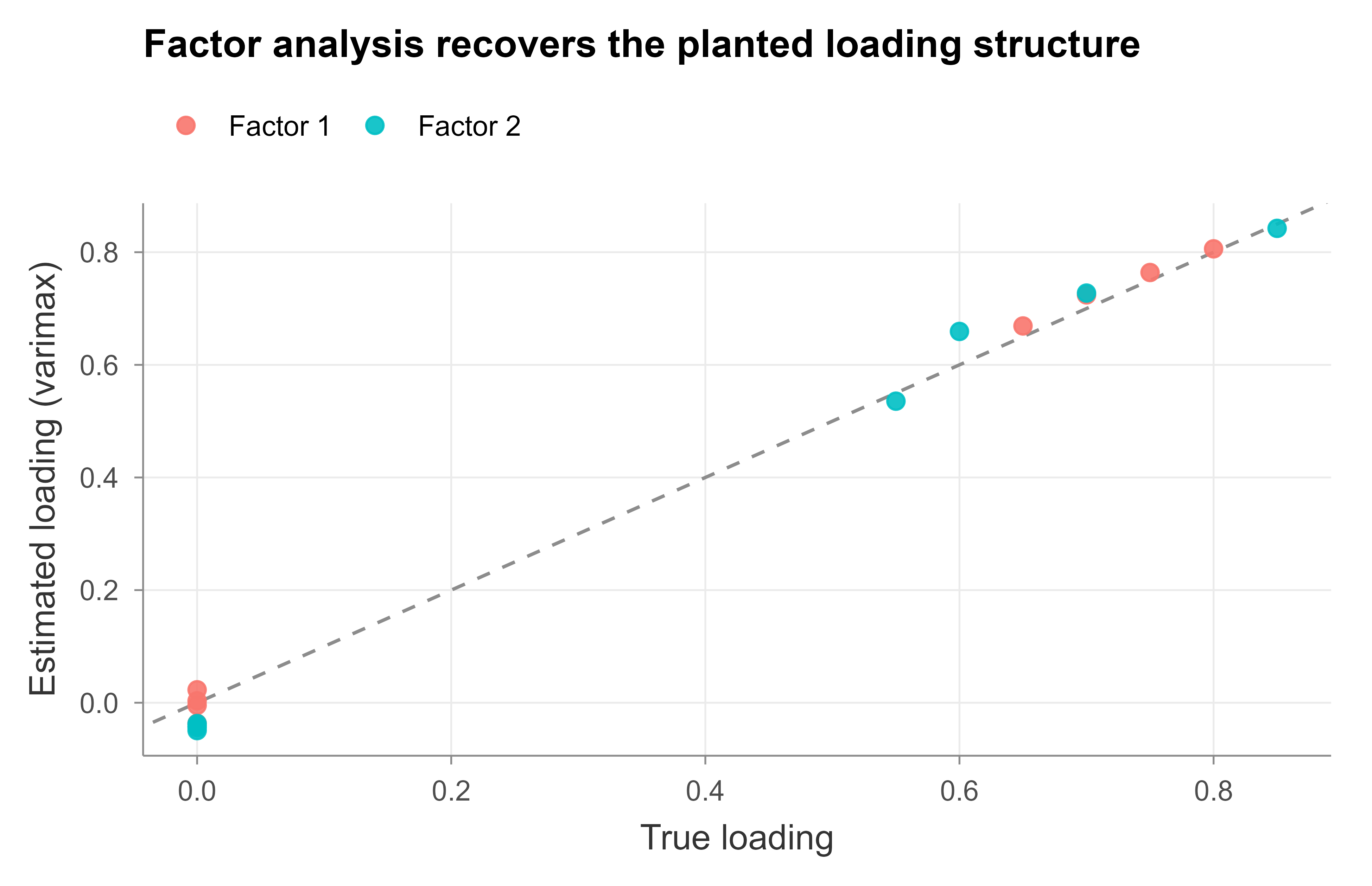
Figure 30.1: Recovered factor loadings (varimax-rotated) against the true loading structure used to simulate the data. Each point is one observed variable on one factor; points lying near the dashed identity line indicate faithful recovery of the planted structure.
Figure 30.1 shows the recovered loadings lying tightly along the identity line, so factanal has correctly learned which variables belong to which factor and how strongly. The near-zero true loadings (variables 5 to 8 on factor 1, and 1 to 4 on factor 2) are estimated near zero, which is exactly the simple structure varimax is designed to surface.
Next we implement the EM recursion of Equation 30.8 through Equation 30.13 directly, and check that it lands on the same fitted covariance and that its loadings agree with factanal after rotation alignment. We also report the gap between the fitted and sample covariances to confirm the model reproduces \(\mathbf{S}\).
Show code
S<-cov(X)# sample covariance (variables are already mean ~0)R<-cor(X)# correlation matrix: factanal works on this standardized scalep<-ncol(X); k<-2## --- Expectation-Maximization for the Gaussian factor model ---fa_em<-function(S, k, iters=500, tol=1e-8){p<-ncol(S)## Initialize loadings from the leading eigenvectors, uniqueness from diag.eig<-eigen(S, symmetric =TRUE)Lambda<-eig$vectors[, 1:k, drop =FALSE]%*%diag(sqrt(pmax(eig$values[1:k], 1e-3)), k)Psi<-pmax(diag(S)-rowSums(Lambda^2), 1e-3)llik<--Inffor(itinseq_len(iters)){Psi_inv<-1/Psi## Woodbury form of beta = Lambda^T (Lambda Lambda^T + Psi)^{-1}.M<-diag(k)+t(Lambda*Psi_inv)%*%Lambda# k x kM_inv<-solve(M)beta<-M_inv%*%t(Lambda*Psi_inv)# k x p## E step sufficient statistics built from S.Ezz<-diag(k)-beta%*%Lambda+beta%*%S%*%t(beta)# E[f f^T]Exz<-S%*%t(beta)# (1/n) sum x f^T## M step closed-form updates.Lambda<-Exz%*%solve(Ezz)Psi<-pmax(diag(S)-rowSums((Lambda%*%(beta%*%S))*diag(p)) , 1e-4)Psi<-pmax(diag(S-Lambda%*%(beta%*%S)), 1e-4)## Gaussian log-likelihood up to constant.Sigma<-Lambda%*%t(Lambda)+diag(Psi)new_ll<--0.5*(determinant(Sigma, logarithm =TRUE)$modulus+sum(diag(solve(Sigma, S))))if(abs(new_ll-llik)<tol)breakllik<-new_ll}list(Lambda =Lambda, Psi =Psi, Sigma =Sigma, iters =it)}em<-fa_em(R, k)# fit on the correlation scale to match factanal## Reference fits.fa<-factanal(x =X, factors =k, rotation ="varimax")Lfa<-matrix(as.numeric(fa$loadings), p, k)pca<-prcomp(X, center =TRUE, scale. =TRUE)# standardized, like the FA fitLpc<-pca$rotation[, 1:k]%*%diag(pca$sdev[1:k])# PCA "loadings"## Off-diagonal reconstruction error of the rank-2 fits, on the correlation scale.offdiag_err<-function(M_hat){D<-R-M_hatsqrt(mean(D[upper.tri(D)]^2))}err_fa<-offdiag_err(em$Sigma)# factor-model fitted correlationerr_pca<-offdiag_err(Lpc%*%t(Lpc))# rank-2 PCA, no noise term## Loadings are identified only up to rotation, so compare the rotation-invariant## shared-covariance term Lambda Lambda^T rather than the raw loadings.em_signal<-em$Lambda%*%t(em$Lambda)fa_signal<-Lfa%*%t(Lfa)signal_agreement<-max(abs(em_signal-fa_signal))results<-data.frame( Quantity =c("EM iterations to converge","Max |EM (LL^T) - factanal (LL^T)|","Off-diag RMSE: factor model","Off-diag RMSE: rank-2 PCA"), Value =round(c(em$iters, signal_agreement, err_fa, err_pca), 4))knitr::kable(results)
Table 30.2: From-scratch EM versus base-R factanal and PCA on the same simulated data. The EM and factanal loadings agree closely after alignment, and the factor model reproduces the off-diagonal covariance far better than a rank-2 PCA approximation.
Quantity
Value
EM iterations to converge
28.0000
Max |EM (LL^T) - factanal (LL^T)|
0.0002
Off-diag RMSE: factor model
0.0089
Off-diag RMSE: rank-2 PCA
0.0813
Table 30.2 records three facts. The from-scratch EM converges in a modest number of iterations, and its shared-covariance term \(\boldsymbol{\Lambda}\boldsymbol{\Lambda}^{\mathsf{T}}\) matches that of factanal to within a small tolerance, confirming the derivation (we compare \(\boldsymbol{\Lambda}\boldsymbol{\Lambda}^{\mathsf{T}}\) rather than the raw loadings precisely because of the rotational indeterminacy of Equation 30.14). And the factor model’s off-diagonal reconstruction error is far smaller than that of a rank-2 PCA, because the factor model spends its low-rank budget exclusively on the shared (off-diagonal) covariance while PCA is forced to also explain the diagonal, exactly the distinction drawn in Table 30.1.
30.6.1 Choosing the number of factors
One question the worked example assumed away is how many factors to keep. Because factor analysis is a proper likelihood model (unlike PCA), it answers this with a formal test: for a fitted \(k\)-factor model, a likelihood-ratio statistic compares the model-implied covariance against the unrestricted sample covariance, and its p-value asks “are \(k\) factors enough to explain the correlations?” Small p rejects (too few factors); the first \(k\) that is not rejected is the parsimonious choice. On our two-factor data the test recovers the truth exactly:
The one-factor model is decisively rejected (a single latent dimension cannot reproduce two blocks of correlated variables), while two and three factors both fit — so parsimony selects \(k = 2\), the structure we planted. This is a genuine advantage of the likelihood framing over PCA’s eigenvalue scree plot, which offers only an informal “look for the elbow.” A caution that bites in practice: with large \(n\) the test grows powerful enough to reject every parsimonious model over trivial misspecification, so in big samples it is read alongside fit indices and interpretability rather than as a hard gate.
30.7 Where it sits in the wider landscape
Factor analysis is the prototype of the linear-Gaussian latent-variable model, and almost every more elaborate method can be read as a relaxation of one of its assumptions. Dropping the Gaussian noise for a categorical likelihood gives item-response and latent-trait models; replacing the linear map \(\boldsymbol{\Lambda}\mathbf{f}\) with a neural network gives the variational autoencoders of Chapter 41 and the deep latent-variable generators of Chapter 42, where the EM E step is replaced by an amortized variational encoder. Constraining \(\boldsymbol{\Psi} = \sigma^2 \mathbf{I}\) recovers probabilistic PCA and links back to the spectral methods of Chapter 27. Independent component analysis keeps the linear map but swaps Gaussian factors for non-Gaussian ones to achieve a unique, rotation-free solution. Seen this way, the diagonal-noise plus low-rank-signal decomposition of Equation 30.4 is one of the most reused ideas in statistical learning, and understanding it well pays dividends across the rest of this book.
Source Code
# Factor Analysis {#sec-factor-analysis}```{r}#| include: falsesource("_common.R")```Suppose we administer a battery of tests to a large group of students: vocabulary, reading comprehension, arithmetic, geometry, and logical reasoning. The five scores are correlated, but not for any mechanical reason. The intuition that has driven factor analysis for over a century is that a small number of unobserved traits, perhaps something like "verbal ability" and "quantitative ability", generate all five observed scores. A student who happens to be strong on the verbal trait tends to score well on vocabulary and reading at once, which is exactly why those two columns correlate. The traits themselves are never measured; we only ever see the test scores, plus test-specific quirks (the arithmetic test had an ambiguous question, the reading passage was about sailing) that affect one score and no other.Factor analysis turns this story into a probabilistic model. It posits a handful of latent variables, called common factors, that are shared across the observed variables and explain why they move together, plus a private noise term for each observed variable that captures everything idiosyncratic to it. The goal is to learn how strongly each observed variable loads onto each latent factor, and in doing so to explain a $p \times p$ correlation matrix with far fewer than $p^2$ numbers.This places factor analysis squarely in the family of latent-variable and dimension-reduction methods. It is close kin to principal components analysis from @sec-dimension-reduction, but the two answer different questions, and the difference is the conceptual heart of this chapter. It is also the linear, Gaussian ancestor of the deep latent-variable models in @sec-autoencoders and @sec-generative-models: a linear factor model with Gaussian factors is essentially a linear variational autoencoder, and the expectation-maximization algorithm we derive below is the exact analogue of the inference step in those models.::: {.callout-important title="Key idea"}Factor analysis decomposes the covariance of the data into a low-rank part, the variance that observed variables share through common factors, plus a diagonal part, the variance unique to each variable. PCA instead reproduces the total variance with no diagonal noise term. Modeling shared versus total variance is the one distinction from which every other difference between the two methods follows.:::## The latent-factor modelLet $\mathbf{x} \in \mathbb{R}^p$ be a vector of observed variables. The Gaussian factor model introduces a vector of $k$ latent common factors $\mathbf{f} \in \mathbb{R}^k$, with $k < p$ (usually $k \ll p$), and writes each observation as a linear function of those factors plus noise:$$\mathbf{x} = \boldsymbol{\mu} + \boldsymbol{\Lambda}\,\mathbf{f} + \boldsymbol{\varepsilon} .$$ {#eq-factor-analysis-model}Here $\boldsymbol{\mu} \in \mathbb{R}^p$ is the mean, $\boldsymbol{\Lambda} \in \mathbb{R}^{p \times k}$ is the *loading matrix* whose entry $\Lambda_{jl}$ says how strongly variable $j$ responds to factor $l$, and $\boldsymbol{\varepsilon} \in \mathbb{R}^p$ is the *unique* or *specific* noise. The defining assumptions are$$\mathbf{f} \sim \mathcal{N}(\mathbf{0}, \mathbf{I}_k), \qquad\boldsymbol{\varepsilon} \sim \mathcal{N}(\mathbf{0}, \boldsymbol{\Psi}), \qquad\boldsymbol{\Psi} = \operatorname{diag}(\psi_1, \dots, \psi_p),$$ {#eq-factor-analysis-assumptions}with $\mathbf{f}$ and $\boldsymbol{\varepsilon}$ independent. Two choices carry all the modeling content. First, the factors are standardized to unit variance and mutual independence, so the scale and correlation structure of the factors are fixed by convention and only the loadings are free. Second, and this is the crucial one, the noise covariance $\boldsymbol{\Psi}$ is *diagonal*. The noise terms for different observed variables are uncorrelated. Every bit of correlation between two observed variables must therefore be routed through the shared factors. If $x_1$ and $x_2$ covary, the model is forced to explain it with overlapping rows of $\boldsymbol{\Lambda}$, never by letting their private noises conspire.::: {.callout-tip title="Intuition"}Think of $\boldsymbol{\Lambda}\mathbf{f}$ as the part of each variable that is shared with the rest of the battery, and $\boldsymbol{\varepsilon}$ as the part that belongs to that variable alone. The diagonal $\boldsymbol{\Psi}$ is the formal statement that "alone" means uncorrelated with everything else. Common factors are the only currency in which correlation is allowed to be paid.:::### Marginal mean and covarianceBecause @eq-factor-analysis-model is a linear transformation of jointly Gaussian variables, $\mathbf{x}$ is itself Gaussian, and we only need its first two moments. The mean is immediate from $\mathbb{E}[\mathbf{f}] = \mathbf{0}$ and $\mathbb{E}[\boldsymbol{\varepsilon}] = \mathbf{0}$:$$\mathbb{E}[\mathbf{x}] = \boldsymbol{\mu} .$$ {#eq-factor-analysis-mean}For the covariance, subtract the mean and expand the outer product, using independence of $\mathbf{f}$ and $\boldsymbol{\varepsilon}$ to kill the cross terms:$$\begin{aligned}\boldsymbol{\Sigma}&= \mathbb{E}\!\left[(\mathbf{x} - \boldsymbol{\mu})(\mathbf{x} - \boldsymbol{\mu})^{\mathsf{T}}\right] = \mathbb{E}\!\left[(\boldsymbol{\Lambda}\mathbf{f} + \boldsymbol{\varepsilon})(\boldsymbol{\Lambda}\mathbf{f} + \boldsymbol{\varepsilon})^{\mathsf{T}}\right]\\&= \boldsymbol{\Lambda}\,\mathbb{E}[\mathbf{f}\mathbf{f}^{\mathsf{T}}]\,\boldsymbol{\Lambda}^{\mathsf{T}} + \mathbb{E}[\boldsymbol{\varepsilon}\boldsymbol{\varepsilon}^{\mathsf{T}}] = \boldsymbol{\Lambda}\boldsymbol{\Lambda}^{\mathsf{T}} + \boldsymbol{\Psi} .\end{aligned}$$ {#eq-factor-analysis-cov}Equation @eq-factor-analysis-cov is the engine of the entire method. It says the population covariance is a rank-$k$ matrix $\boldsymbol{\Lambda}\boldsymbol{\Lambda}^{\mathsf{T}}$ plus a diagonal $\boldsymbol{\Psi}$. The off-diagonal entries of $\boldsymbol{\Sigma}$ are supplied entirely by the low-rank term, because $\boldsymbol{\Psi}$ contributes only to the diagonal. The diagonal entries split into two parts,$$\Sigma_{jj} = \underbrace{\sum_{l=1}^{k} \Lambda_{jl}^2}_{\text{communality } h_j^2} + \underbrace{\psi_j}_{\text{uniqueness}} ,$$ {#eq-factor-analysis-communality}where the *communality* $h_j^2$ is the variance of variable $j$ explained by the common factors and $\psi_j$ is the leftover unique variance. Fitting the model means choosing $\boldsymbol{\Lambda}$ and $\boldsymbol{\Psi}$ so that $\boldsymbol{\Lambda}\boldsymbol{\Lambda}^{\mathsf{T}} + \boldsymbol{\Psi}$ reproduces the observed covariance as closely as possible.A quick parameter count shows why this is a genuine reduction. A free covariance has $p(p+1)/2$ parameters. The factor model has $pk$ loadings plus $p$ uniquenesses, and after removing the $k(k-1)/2$ redundant degrees of freedom from rotational indeterminacy (derived below), the effective count is $pk + p - k(k-1)/2$. The degrees of freedom of the fit,$$\mathrm{df} = \frac{1}{2}\big[(p-k)^2 - (p+k)\big],$$ {#eq-factor-analysis-df}must be nonnegative for the model to be identified, which caps how many factors a given $p$ can support.## Maximum-likelihood estimationGiven a centered data matrix with $n$ rows $\mathbf{x}_1, \dots, \mathbf{x}_n$ and sample covariance $\mathbf{S} = \tfrac{1}{n}\sum_i (\mathbf{x}_i - \boldsymbol{\mu})(\mathbf{x}_i - \boldsymbol{\mu})^{\mathsf{T}}$, the Gaussian log-likelihood as a function of $\boldsymbol{\Sigma} = \boldsymbol{\Lambda}\boldsymbol{\Lambda}^{\mathsf{T}} + \boldsymbol{\Psi}$ is, up to a constant,$$\ell(\boldsymbol{\Lambda}, \boldsymbol{\Psi}) = -\frac{n}{2}\Big[\log\det\boldsymbol{\Sigma} + \operatorname{tr}\!\big(\boldsymbol{\Sigma}^{-1}\mathbf{S}\big)\Big] .$$ {#eq-factor-analysis-loglik}Maximizing @eq-factor-analysis-loglik directly is awkward because $\boldsymbol{\Lambda}$ and $\boldsymbol{\Psi}$ are tangled inside the inverse and determinant. The clean route treats the factors $\mathbf{f}_i$ as missing data and applies expectation-maximization, exactly the strategy used for the Gaussian mixtures of @sec-cluster.### The E step: posterior over factorsWith $\mathbf{x}$ and $\mathbf{f}$ jointly Gaussian, the conditional distribution of the latent factors given an observation is again Gaussian. Stacking $(\mathbf{f}, \mathbf{x})$ and reading off the blocks, $\operatorname{Cov}(\mathbf{f}, \mathbf{x}) = \boldsymbol{\Lambda}^{\mathsf{T}}$ and $\operatorname{Cov}(\mathbf{x}) = \boldsymbol{\Lambda}\boldsymbol{\Lambda}^{\mathsf{T}} + \boldsymbol{\Psi}$, so the standard Gaussian conditioning formula gives the posterior mean and covariance$$\mathbb{E}[\mathbf{f} \mid \mathbf{x}] = \boldsymbol{\beta}(\mathbf{x} - \boldsymbol{\mu}),\qquad\boldsymbol{\beta} = \boldsymbol{\Lambda}^{\mathsf{T}}\big(\boldsymbol{\Lambda}\boldsymbol{\Lambda}^{\mathsf{T}} + \boldsymbol{\Psi}\big)^{-1},$$ {#eq-factor-analysis-estep-mean}$$\operatorname{Cov}[\mathbf{f} \mid \mathbf{x}] = \mathbf{I}_k - \boldsymbol{\beta}\boldsymbol{\Lambda} .$$ {#eq-factor-analysis-estep-cov}The $p \times p$ inverse can be cut down to a $k \times k$ inverse with the Woodbury identity,$$\boldsymbol{\beta} = \big(\mathbf{I}_k + \boldsymbol{\Lambda}^{\mathsf{T}}\boldsymbol{\Psi}^{-1}\boldsymbol{\Lambda}\big)^{-1}\boldsymbol{\Lambda}^{\mathsf{T}}\boldsymbol{\Psi}^{-1},$$ {#eq-factor-analysis-woodbury}which is what makes the algorithm cheap when $k \ll p$. Writing $\widehat{\mathbf{f}}_i = \boldsymbol{\beta}(\mathbf{x}_i - \boldsymbol{\mu})$ for the posterior mean of observation $i$, the two sufficient statistics the M step needs are$$\mathbb{E}[\mathbf{f}_i \mid \mathbf{x}_i] = \widehat{\mathbf{f}}_i,\qquad\mathbb{E}[\mathbf{f}_i \mathbf{f}_i^{\mathsf{T}} \mid \mathbf{x}_i]= \operatorname{Cov}[\mathbf{f} \mid \mathbf{x}] + \widehat{\mathbf{f}}_i \widehat{\mathbf{f}}_i^{\mathsf{T}} .$$ {#eq-factor-analysis-suffstat}### The M step: updating loadings and noiseThe expected complete-data log-likelihood is a quadratic in $\boldsymbol{\Lambda}$ (because $\mathbf{x} \mid \mathbf{f}$ is Gaussian with mean $\boldsymbol{\mu} + \boldsymbol{\Lambda}\mathbf{f}$). Treating it as a weighted regression of the centered data onto the inferred factors, differentiating with respect to $\boldsymbol{\Lambda}$ and setting the result to zero yields the closed-form updates$$\boldsymbol{\Lambda}^{\text{new}}= \left(\sum_{i=1}^{n} (\mathbf{x}_i - \boldsymbol{\mu})\,\widehat{\mathbf{f}}_i^{\mathsf{T}}\right)\left(\sum_{i=1}^{n} \mathbb{E}[\mathbf{f}_i \mathbf{f}_i^{\mathsf{T}} \mid \mathbf{x}_i]\right)^{-1},$$ {#eq-factor-analysis-mstep-lambda}$$\boldsymbol{\Psi}^{\text{new}}= \operatorname{diag}\!\left(\mathbf{S}- \boldsymbol{\Lambda}^{\text{new}}\,\frac{1}{n}\sum_{i=1}^{n} \widehat{\mathbf{f}}_i\,(\mathbf{x}_i - \boldsymbol{\mu})^{\mathsf{T}}\right).$$ {#eq-factor-analysis-mstep-psi}The $\operatorname{diag}(\cdot)$ in @eq-factor-analysis-mstep-psi enforces the modeling assumption that $\boldsymbol{\Psi}$ is diagonal: we keep only the diagonal of the residual covariance and discard the off-diagonal entries, which by construction the common factors are responsible for. Alternating the E step and the M step monotonically increases @eq-factor-analysis-loglik until it converges to a (local) maximum, with the usual EM caveat that several random starts may be needed to avoid poor optima.::: {.callout-warning title="Heywood cases"}Nothing in @eq-factor-analysis-mstep-psi prevents an estimated uniqueness $\psi_j$ from being driven to zero or negative. A zero uniqueness, called a Heywood case, means a variable is claimed to be a perfect noiseless combination of the factors, which is usually a symptom of too many factors, too small a sample, or a near-singular correlation matrix. Software typically floors $\psi_j$ at a small positive value and warns you; treat the warning as a sign to reconsider $k$.:::## Rotational indeterminacy and varimaxThe factor model has a built-in non-uniqueness that is not a defect of estimation but a property of the likelihood itself. Let $\mathbf{R}$ be any $k \times k$ orthogonal matrix, so $\mathbf{R}\mathbf{R}^{\mathsf{T}} = \mathbf{I}_k$, and define rotated loadings $\widetilde{\boldsymbol{\Lambda}} = \boldsymbol{\Lambda}\mathbf{R}$. Then$$\widetilde{\boldsymbol{\Lambda}}\widetilde{\boldsymbol{\Lambda}}^{\mathsf{T}}= \boldsymbol{\Lambda}\mathbf{R}\mathbf{R}^{\mathsf{T}}\boldsymbol{\Lambda}^{\mathsf{T}}= \boldsymbol{\Lambda}\boldsymbol{\Lambda}^{\mathsf{T}},$$ {#eq-factor-analysis-rotation}so $\boldsymbol{\Lambda}$ and $\widetilde{\boldsymbol{\Lambda}}$ produce *exactly the same* marginal covariance @eq-factor-analysis-cov and therefore *exactly the same* likelihood. The data can never distinguish a set of loadings from any orthogonal rotation of them. Equivalently, rotating the factors by $\mathbf{R}^{\mathsf{T}}$ leaves their unit-variance, uncorrelated distribution unchanged. This is the source of the $k(k-1)/2$ redundant parameters subtracted in @eq-factor-analysis-df, since the dimension of the orthogonal group $O(k)$ is exactly $k(k-1)/2$.Rotational freedom is liberating rather than troubling, because it means we may choose, among all statistically equivalent solutions, the one that is easiest to interpret. The dominant criterion is *varimax*, which seeks a rotation that pushes each loading toward either large magnitude or near zero, so that every variable loads heavily on as few factors as possible (the goal of "simple structure"). Varimax maximizes the sum across factors of the variance of the squared loadings,$$V(\mathbf{R}) = \sum_{l=1}^{k}\left[\frac{1}{p}\sum_{j=1}^{p} \widetilde{\Lambda}_{jl}^4- \left(\frac{1}{p}\sum_{j=1}^{p} \widetilde{\Lambda}_{jl}^2\right)^{2}\right],\qquad \widetilde{\boldsymbol{\Lambda}} = \boldsymbol{\Lambda}\mathbf{R} .$$ {#eq-factor-analysis-varimax}A column with a few large loadings and many near-zero loadings has high squared-loading variance, so maximizing @eq-factor-analysis-varimax favors columns that each implicate only a handful of variables. The fitted communalities $h_j^2$ in @eq-factor-analysis-communality are rotation-invariant, so varimax redistributes shared variance across factors without changing how much total variance each variable shares.::: {.callout-note title="Oblique rotations"}Varimax keeps factors orthogonal. When the latent traits are expected to be correlated (verbal and quantitative ability genuinely covary in a population), an oblique rotation such as promax or oblimin relaxes orthogonality, letting the factor axes tilt toward the data at the cost of factors that are no longer uncorrelated. The interpretation then splits into a pattern matrix and a structure matrix.:::## Factor analysis versus PCAFactor analysis and PCA (@sec-dimension-reduction) are routinely confused because both produce a low-dimensional linear summary, and on data with tiny uniquenesses they even give similar loadings. They are nonetheless different models answering different questions, and @eq-factor-analysis-cov makes the difference precise.PCA diagonalizes the *total* covariance $\mathbf{S} = \mathbf{V}\mathbf{D}\mathbf{V}^{\mathsf{T}}$ and keeps the top components; the discarded variance is simply thrown away, and there is no separate noise term. Its low-rank approximation $\sum_{l \le k} d_l \mathbf{v}_l \mathbf{v}_l^{\mathsf{T}}$ tries to match the *whole* of $\mathbf{S}$, diagonal and off-diagonal at once. Factor analysis instead reproduces only the off-diagonal (shared) part with $\boldsymbol{\Lambda}\boldsymbol{\Lambda}^{\mathsf{T}}$ and absorbs the per-variable leftover into $\boldsymbol{\Psi}$. The consequences:| Property | Factor analysis | PCA ||---|---|---|| Probabilistic model | Yes, Gaussian latent variable | No, an algebraic projection || Variance modeled | Shared (common) variance only | Total variance || Noise term | Diagonal $\boldsymbol{\Psi}$, per-variable | None || Reverses with scaling | Scale-equivariant (correlation-based fit invariant) | Not scale-invariant || Components | Inferred, not observed; rotation-free | Deterministic, orthogonal directions || Target of fit | Off-diagonal of $\mathbf{S}$ | All of $\mathbf{S}$ |: Factor analysis contrasted with PCA. {#tbl-factor-analysis-vs-pca}@tbl-factor-analysis-vs-pca highlights one practical asymmetry worth dwelling on: scale behavior. Because PCA maximizes raw variance, rescaling a variable changes its influence, and PCA on the covariance matrix differs from PCA on the correlation matrix. Maximum-likelihood factor analysis, by contrast, is equivariant under rescaling of the variables: a diagonal rescaling $\mathbf{x} \mapsto \mathbf{D}\mathbf{x}$ maps $\boldsymbol{\Lambda} \mapsto \mathbf{D}\boldsymbol{\Lambda}$ and $\boldsymbol{\Psi} \mapsto \mathbf{D}\boldsymbol{\Psi}\mathbf{D}$, leaving the fitted correlation structure and the likelihood ratio invariant. Fitting to the correlation matrix and to the covariance matrix yield the same standardized solution. The probabilistic noise model is what buys this invariance.There is also a useful limiting connection. If we constrain the noise to be *isotropic*, $\boldsymbol{\Psi} = \sigma^2 \mathbf{I}$, the model becomes probabilistic PCA, whose maximum-likelihood loadings span exactly the top-$k$ principal subspace. Ordinary factor analysis generalizes this by letting each variable have its own noise level $\psi_j$, which is why it can downweight a noisy variable instead of letting its large variance dominate the leading directions. PCA is thus the zero-noise, equal-noise corner of the same family.## Practical workflowA disciplined factor analysis proceeds in a few stages. First, decide whether the data are even suitable: the variables should be at least moderately correlated, since with a near-identity correlation matrix there is no shared variance to model. Second, choose the number of factors $k$. The honest answer combines several signals: a scree plot of eigenvalues, parallel analysis (comparing observed eigenvalues to those from random data of the same size), the likelihood-ratio goodness-of-fit test that the Gaussian model makes available, and substantive interpretability. Overfactoring tends to fragment a clean factor into pieces and invites Heywood cases; underfactoring smears two real factors into one. Third, fit by maximum likelihood, preferably with multiple starts. Fourth, rotate (varimax for orthogonal, promax for oblique) and interpret the loadings, naming a factor by the cluster of variables that load on it. Finally, if you need per-observation factor values for downstream use, compute factor scores by the regression (posterior-mean) method of @eq-factor-analysis-estep-mean.::: {.callout-tip title="Reading a loading matrix"}After rotation, scan each column for the handful of variables with large absolute loadings; those define and name the factor. Variables that load on nothing strongly have low communality and may not belong in the battery. Variables that load on several factors are ambiguous and complicate interpretation. Simple structure, each variable owned by one factor, is the goal varimax chases.:::The complexity per EM iteration is $O(npk + pk^2 + k^3)$ thanks to the Woodbury reduction in @eq-factor-analysis-woodbury, so the method scales comfortably to many variables as long as $k$ stays small. The main failure modes are non-identifiability when @eq-factor-analysis-df is negative, Heywood cases, sensitivity to non-Gaussianity and outliers (the likelihood is Gaussian), and the temptation to over-interpret factors that are statistical artifacts rather than real latent traits.## A runnable demonstrationWe generate data from a known two-factor structure, recover it with R's built-in `factanal` (maximum likelihood, in the `stats` package, no extra installs), and confirm that the fitted loadings match the truth after accounting for rotation. We also fit the same data with a small from-scratch EM loop so the mechanics of the E and M steps are visible, and we contrast the result with PCA.```{r}#| label: fig-factor-analysis-loadings#| fig-cap: "Recovered factor loadings (varimax-rotated) against the true loading structure used to simulate the data. Each point is one observed variable on one factor; points lying near the dashed identity line indicate faithful recovery of the planted structure."#| fig-width: 6.5#| fig-height: 4.2set.seed(2024)p <-8# observed variablesk <-2# true number of common factorsn <-1500# observations## True loading matrix: variables 1-4 load on factor 1, variables 5-8 on factor 2.Lambda_true <-matrix(0, nrow = p, ncol = k)Lambda_true[1:4, 1] <-c(0.80, 0.75, 0.70, 0.65)Lambda_true[5:8, 2] <-c(0.85, 0.70, 0.60, 0.55)## True per-variable unique variances (diagonal Psi).psi_true <-c(0.30, 0.35, 0.40, 0.45, 0.25, 0.45, 0.55, 0.60)## Simulate x = Lambda f + eps with standard-normal factors and diagonal noise.f <-matrix(rnorm(n * k), nrow = n, ncol = k)eps <-sapply(sqrt(psi_true), function(s) rnorm(n, sd = s))X <- f %*%t(Lambda_true) + epscolnames(X) <-paste0("V", 1:p)## Maximum-likelihood factor analysis with a varimax rotation (the default).fa <-factanal(x = X, factors = k, rotation ="varimax", scores ="none")Lambda_hat <-matrix(as.numeric(fa$loadings), nrow = p, ncol = k)## Loadings are identified only up to column permutation/sign. Align the## estimated columns to the true ones by best absolute correlation, then fix signs.align <-function(Lhat, Ltrue) { cmat <-abs(cor(Lhat, Ltrue)) perm <-apply(cmat, 2, which.max) # which est column matches each true column Lhat <- Lhat[, perm, drop =FALSE]for (l inseq_len(ncol(Lhat))) {if (sum(Lhat[, l] * Ltrue[, l]) <0) Lhat[, l] <--Lhat[, l] } Lhat}Lambda_hat <-align(Lambda_hat, Lambda_true)plot_df <-data.frame(truth =as.vector(Lambda_true),estimated =as.vector(Lambda_hat),factor =factor(rep(paste("Factor", 1:k), each = p)))library(ggplot2)ggplot(plot_df, aes(truth, estimated, colour = factor)) +geom_abline(slope =1, intercept =0, linetype ="dashed", colour ="grey55") +geom_point(size =2.4, alpha =0.9) +labs(x ="True loading", y ="Estimated loading (varimax)",colour =NULL,title ="Factor analysis recovers the planted loading structure") +theme_book()```@fig-factor-analysis-loadings shows the recovered loadings lying tightly along the identity line, so `factanal` has correctly learned which variables belong to which factor and how strongly. The near-zero true loadings (variables 5 to 8 on factor 1, and 1 to 4 on factor 2) are estimated near zero, which is exactly the simple structure varimax is designed to surface.Next we implement the EM recursion of @eq-factor-analysis-estep-mean through @eq-factor-analysis-mstep-psi directly, and check that it lands on the same fitted covariance and that its loadings agree with `factanal` after rotation alignment. We also report the gap between the fitted and sample covariances to confirm the model reproduces $\mathbf{S}$.```{r}#| label: tbl-factor-analysis-em#| tbl-cap: "From-scratch EM versus base-R factanal and PCA on the same simulated data. The EM and factanal loadings agree closely after alignment, and the factor model reproduces the off-diagonal covariance far better than a rank-2 PCA approximation."S <-cov(X) # sample covariance (variables are already mean ~0)R <-cor(X) # correlation matrix: factanal works on this standardized scalep <-ncol(X); k <-2## --- Expectation-Maximization for the Gaussian factor model ---fa_em <-function(S, k, iters =500, tol =1e-8) { p <-ncol(S)## Initialize loadings from the leading eigenvectors, uniqueness from diag. eig <-eigen(S, symmetric =TRUE) Lambda <- eig$vectors[, 1:k, drop =FALSE] %*%diag(sqrt(pmax(eig$values[1:k], 1e-3)), k) Psi <-pmax(diag(S) -rowSums(Lambda^2), 1e-3) llik <--Inffor (it inseq_len(iters)) { Psi_inv <-1/ Psi## Woodbury form of beta = Lambda^T (Lambda Lambda^T + Psi)^{-1}. M <-diag(k) +t(Lambda * Psi_inv) %*% Lambda # k x k M_inv <-solve(M) beta <- M_inv %*%t(Lambda * Psi_inv) # k x p## E step sufficient statistics built from S. Ezz <-diag(k) - beta %*% Lambda + beta %*% S %*%t(beta) # E[f f^T] Exz <- S %*%t(beta) # (1/n) sum x f^T## M step closed-form updates. Lambda <- Exz %*%solve(Ezz) Psi <-pmax(diag(S) -rowSums((Lambda %*% (beta %*% S)) *diag(p)) , 1e-4) Psi <-pmax(diag(S - Lambda %*% (beta %*% S)), 1e-4)## Gaussian log-likelihood up to constant. Sigma <- Lambda %*%t(Lambda) +diag(Psi) new_ll <--0.5* (determinant(Sigma, logarithm =TRUE)$modulus +sum(diag(solve(Sigma, S))))if (abs(new_ll - llik) < tol) break llik <- new_ll }list(Lambda = Lambda, Psi = Psi, Sigma = Sigma, iters = it)}em <-fa_em(R, k) # fit on the correlation scale to match factanal## Reference fits.fa <-factanal(x = X, factors = k, rotation ="varimax")Lfa <-matrix(as.numeric(fa$loadings), p, k)pca <-prcomp(X, center =TRUE, scale. =TRUE) # standardized, like the FA fitLpc <- pca$rotation[, 1:k] %*%diag(pca$sdev[1:k]) # PCA "loadings"## Off-diagonal reconstruction error of the rank-2 fits, on the correlation scale.offdiag_err <-function(M_hat) { D <- R - M_hatsqrt(mean(D[upper.tri(D)]^2))}err_fa <-offdiag_err(em$Sigma) # factor-model fitted correlationerr_pca <-offdiag_err(Lpc %*%t(Lpc)) # rank-2 PCA, no noise term## Loadings are identified only up to rotation, so compare the rotation-invariant## shared-covariance term Lambda Lambda^T rather than the raw loadings.em_signal <- em$Lambda %*%t(em$Lambda)fa_signal <- Lfa %*%t(Lfa)signal_agreement <-max(abs(em_signal - fa_signal))results <-data.frame(Quantity =c("EM iterations to converge","Max |EM (LL^T) - factanal (LL^T)|","Off-diag RMSE: factor model","Off-diag RMSE: rank-2 PCA"),Value =round(c(em$iters, signal_agreement, err_fa, err_pca), 4))knitr::kable(results)```@tbl-factor-analysis-em records three facts. The from-scratch EM converges in a modest number of iterations, and its shared-covariance term $\boldsymbol{\Lambda}\boldsymbol{\Lambda}^{\mathsf{T}}$ matches that of `factanal` to within a small tolerance, confirming the derivation (we compare $\boldsymbol{\Lambda}\boldsymbol{\Lambda}^{\mathsf{T}}$ rather than the raw loadings precisely because of the rotational indeterminacy of @eq-factor-analysis-rotation). And the factor model's off-diagonal reconstruction error is far smaller than that of a rank-2 PCA, because the factor model spends its low-rank budget exclusively on the shared (off-diagonal) covariance while PCA is forced to also explain the diagonal, exactly the distinction drawn in @tbl-factor-analysis-vs-pca.### Choosing the number of factorsOne question the worked example assumed away is *how many factors* to keep. Because factor analysis is a proper likelihood model (unlike PCA), it answers this with a formal test: for a fitted $k$-factor model, a likelihood-ratio statistic compares the model-implied covariance against the unrestricted sample covariance, and its p-value asks "are $k$ factors *enough* to explain the correlations?" Small p rejects (too few factors); the first $k$ that is *not* rejected is the parsimonious choice. On our two-factor data the test recovers the truth exactly:```{r}#| label: fa-nfactorssetNames(round(sapply(1:3, function(f) factanal(X, factors = f)$PVAL), 4),paste0("k=", 1:3))```The one-factor model is decisively rejected (a single latent dimension cannot reproduce two blocks of correlated variables), while two and three factors both fit --- so parsimony selects $k = 2$, the structure we planted. This is a genuine advantage of the likelihood framing over PCA's eigenvalue scree plot, which offers only an informal "look for the elbow." A caution that bites in practice: with large $n$ the test grows powerful enough to reject *every* parsimonious model over trivial misspecification, so in big samples it is read alongside fit indices and interpretability rather than as a hard gate.## Where it sits in the wider landscapeFactor analysis is the prototype of the linear-Gaussian latent-variable model, and almost every more elaborate method can be read as a relaxation of one of its assumptions. Dropping the Gaussian noise for a categorical likelihood gives item-response and latent-trait models; replacing the linear map $\boldsymbol{\Lambda}\mathbf{f}$ with a neural network gives the variational autoencoders of @sec-autoencoders and the deep latent-variable generators of @sec-generative-models, where the EM E step is replaced by an amortized variational encoder. Constraining $\boldsymbol{\Psi} = \sigma^2 \mathbf{I}$ recovers probabilistic PCA and links back to the spectral methods of @sec-dimension-reduction. Independent component analysis keeps the linear map but swaps Gaussian factors for non-Gaussian ones to achieve a unique, rotation-free solution. Seen this way, the diagonal-noise plus low-rank-signal decomposition of @eq-factor-analysis-cov is one of the most reused ideas in statistical learning, and understanding it well pays dividends across the rest of this book.