Imagine standing in a crowded room where several people speak at once. Two microphones placed in different corners each pick up a different blend of all the voices. From those two mixed recordings, can you reconstruct what each individual speaker said? Your ear does something like this effortlessly, which is why the problem is known as the cocktail-party problem. Independent component analysis (ICA) is the statistical machinery that solves it without knowing anything about the voices or the room: it takes the mixed signals and pulls them back apart into the underlying sources.
This is a deceptively hard task. We never observe the original voices, and we do not know how they were combined. We only see the mixtures. The remarkable claim of ICA is that, under one structural assumption (the sources are statistically independent and at most one of them is Gaussian), the unmixing can be recovered up to harmless ambiguities of scale and ordering. The single idea that makes this possible is that mixing makes signals look more Gaussian, so undoing the mixing amounts to searching for directions in which the data look as non-Gaussian as possible.
ICA belongs to the same family of unsupervised, linear factorizations as principal components analysis (see Chapter 27), and it is often introduced right after it. The two methods look superficially similar (both write the data as linear combinations of latent variables), but they optimize fundamentally different criteria. PCA seeks directions that are uncorrelated and capture maximal variance; ICA seeks directions that are statistically independent. As we will see, independence is a much stronger requirement than uncorrelatedness, and it is exactly what lets ICA separate sources that PCA cannot.
Key idea
PCA decorrelates (removes second-order, linear dependence) and orders directions by variance. ICA goes further and makes the recovered components statistically independent, which requires using information beyond the covariance matrix, namely the non-Gaussian structure of the data.
28.1 The Mixing Model
Let there be \(m\) unobserved source signals collected into a random vector \(\mathbf{s} = (s_1, \dots, s_m)^\top\). We observe \(m\) mixtures \(\mathbf{x} = (x_1, \dots, x_m)^\top\), each a linear combination of the sources. In matrix form the generative model is
where \(\mathbf{A}\) is an unknown invertible \(m \times m\) mixing matrix. In the cocktail-party picture, \(s_j\) is the \(j\)th speaker, \(x_i\) is the \(i\)th microphone, and \(A_{ij}\) encodes how loudly speaker \(j\) reaches microphone \(i\). Given a sample of \(n\) observed vectors, stacked as the rows of an \(n \times m\) matrix \(\mathbf{X}\), the goal is to estimate an unmixing matrix \(\mathbf{W} \approx \mathbf{A}^{-1}\) so that
and that at most one of the \(p_j\) is Gaussian. We also assume the sources have zero mean (we can always center the data) and, without loss of generality, unit variance, because any scaling of a source can be absorbed into the corresponding column of \(\mathbf{A}\).
The two unavoidable ambiguities
ICA can never recover the scale or the order of the sources. If \(\mathbf{P}\) is a permutation matrix and \(\mathbf{D}\) a nonzero diagonal matrix, then \(\mathbf{A}\mathbf{D}^{-1}\mathbf{P}^{-1}\) mixing the rescaled, reordered sources \(\mathbf{P}\mathbf{D}\mathbf{s}\) produces exactly the same observations \(\mathbf{x}\). We fix scale by setting unit variance and accept that the labelling and the sign of each component are arbitrary. Everything else is identifiable.
28.1.1 Why independence and non-Gaussianity identify the sources
The single deepest fact in ICA is that Gaussian sources cannot be separated, while non-Gaussian ones can. Understanding why explains the whole method.
Suppose the sources are jointly Gaussian, independent, with unit variance, so \(\mathbf{s} \sim \mathcal{N}(\mathbf{0}, \mathbf{I})\). Then \(\mathbf{x} = \mathbf{A}\mathbf{s} \sim \mathcal{N}(\mathbf{0}, \mathbf{A}\mathbf{A}^\top)\). Now take any orthogonal matrix \(\mathbf{Q}\) (so \(\mathbf{Q}\mathbf{Q}^\top = \mathbf{I}\)) and define a rotated set of sources \(\mathbf{s}' = \mathbf{Q}\mathbf{s}\). Because the standard Gaussian is rotationally symmetric, \(\mathbf{s}'\) is also\(\mathcal{N}(\mathbf{0}, \mathbf{I})\) with independent components, and the alternative mixing matrix \(\mathbf{A}' = \mathbf{A}\mathbf{Q}^\top\) gives
The pair \((\mathbf{A}', \mathbf{s}')\) explains the data exactly as well as \((\mathbf{A}, \mathbf{s})\), and the two are not related by mere permutation and scaling. The model is unidentifiable: any rotation of jointly Gaussian sources is again valid independent Gaussian sources. Second-order statistics (the covariance) are all a Gaussian has, and the covariance is invariant to rotation, so there is simply no information left to pin down the rotation.
Non-Gaussian sources break this symmetry. To see how, consider any linear combination of the observed mixtures, \(y = \mathbf{w}^\top \mathbf{x} = \mathbf{w}^\top \mathbf{A}\,\mathbf{s} = \mathbf{z}^\top \mathbf{s}\), where \(\mathbf{z} = \mathbf{A}^\top \mathbf{w}\). So every candidate unmixing direction \(\mathbf{w}\) produces an output \(y\) that is a weighted sum of the independent sources, \(y = \sum_j z_j s_j\). The classical central limit theorem says that sums of independent random variables tend toward a Gaussian. Therefore a generic mixture \(\sum_j z_j s_j\) is more Gaussian than any single source. The output \(y\) is least Gaussian precisely when the sum collapses onto a single source, that is, when \(\mathbf{z}\) has exactly one nonzero entry. At that point \(y\) equals one of the original \(s_j\) (up to scale). This gives a constructive recipe:
To recover a source, search over directions \(\mathbf{w}\) for the one that makes \(y = \mathbf{w}^\top \mathbf{x}\) as far from Gaussian as possible.
Maximizing non-Gaussianity is the engine of ICA. Everything that follows is about how to measure “non-Gaussianity” with a tractable contrast function and how to optimize it efficiently.
28.2 Whitening: Reducing the Problem to a Rotation
Before searching for the unmixing directions, it pays to preprocess the data so that the remaining work is as simple as possible. The preprocessing is whitening (also called sphering), and it is essentially the same linear-algebra step that powers PCA.
Center the observed data and compute the sample covariance \(\mathbf{C} = \mathbb{E}[\mathbf{x}\mathbf{x}^\top]\). Diagonalize it with its eigendecomposition \(\mathbf{C} = \mathbf{E}\,\boldsymbol{\Lambda}\,\mathbf{E}^\top\), where \(\mathbf{E}\) holds the orthonormal eigenvectors and \(\boldsymbol{\Lambda} = \operatorname{diag}(\lambda_1, \dots, \lambda_m)\) the eigenvalues. Define the whitening matrix
Whitening removes all linear correlation and equalizes variance, which is exactly the second-order, PCA-level structure. What it cannot do is achieve independence, because that involves higher-order statistics. The crucial payoff is that, after whitening, the remaining mixing is a pure rotation. Writing \(\tilde{\mathbf{x}} = \mathbf{V}\mathbf{A}\,\mathbf{s} = \tilde{\mathbf{A}}\,\mathbf{s}\) and using that \(\mathbf{s}\) has identity covariance,
so \(\tilde{\mathbf{A}}\) is orthogonal. The full unmixing problem (\(m^2\) unknowns) has been reduced to finding an orthogonal matrix (\(m(m-1)/2\) free parameters), which is just the search for the rotation that the identifiability argument said Gaussian data could never reveal but non-Gaussian data can. This is why ICA pipelines always whiten first: it halves the work and lets the contrast-function search operate on an orthonormal frame.
Mental model
Whitening turns an arbitrary elliptical cloud into a spherical one. For Gaussian data the sphere looks the same from every angle, which is exactly why no rotation is special. For non-Gaussian data the sphere has lumpy, non-uniform structure, and ICA rotates the axes to line up with the lumps.
To turn “as non-Gaussian as possible” into an objective we can optimize, we need a scalar measure of how far a (zero-mean, unit-variance) random variable \(y\) is from Gaussian. Two classical choices are kurtosis and negentropy.
For a Gaussian, \(\mathbb{E}[y^4] = 3(\mathbb{E}[y^2])^2\), so kurtosis is exactly zero; any nonzero value signals non-Gaussianity. Distributions with positive kurtosis are super-Gaussian (heavy-tailed, spiky, like speech or a Laplace density), while negative kurtosis indicates sub-Gaussian variables (flat-topped, like a uniform distribution or many digital signals). Kurtosis is attractive because it is simple and, for unit-variance variables, behaves nicely under linear combination: if \(y = \sum_j z_j s_j\) with independent \(s_j\) and \(\sum_j z_j^2 = 1\), then
Maximizing \(|\operatorname{kurt}(y)|\) over the unit sphere \(\sum_j z_j^2 = 1\) drives the weight onto a single coordinate (since the quartic \(\sum z_j^4\) is maximized at a vertex), exactly recovering one source. The drawback is statistical: kurtosis depends on fourth moments and is therefore extremely sensitive to outliers, which can dominate the estimate. For this reason practitioners usually prefer negentropy with a robust nonlinearity.
28.3.2 Negentropy
Information theory offers the principled measure. Among all distributions with a fixed variance, the Gaussian has the largest differential entropy. So the entropy gap between \(y\) and a Gaussian of the same variance is a natural, always-nonnegative measure of non-Gaussianity. This is negentropy:
where \(y_{\text{gauss}}\) is Gaussian with the same variance as \(y\). Negentropy is zero if and only if \(y\) is Gaussian and positive otherwise, and unlike kurtosis it uses the entire distribution rather than a single moment, making it statistically well behaved. Its weakness is that it requires the unknown density \(p\). The practical fix, due to Hyvarinen, is the approximation
where \(\nu \sim \mathcal{N}(0,1)\), \(\kappa > 0\) is a constant, and \(G\) is a smooth, slowly growing nonquadratic function. Common choices are \(G(u) = \tfrac{1}{a}\log\cosh(au)\) (so \(g = G' = \tanh(au)\)) and \(G(u) = -e^{-u^2/2}\). These robust contrasts recover the spirit of kurtosis (the special case \(G(u) = u^4\)) while taming the sensitivity to tails, and they lead directly to the FastICA update.
28.4 The FastICA Fixed-Point Algorithm
FastICA finds, on whitened data, a unit vector \(\mathbf{w}\) that maximizes the negentropy approximation in Equation 28.11. We derive its update rule, which is the centerpiece of practical ICA.
28.4.1 Derivation of the fixed point
Work with whitened data \(\tilde{\mathbf{x}}\) and write \(y = \mathbf{w}^\top \tilde{\mathbf{x}}\). Maximizing the approximation in Equation 28.11 with respect to \(\mathbf{w}\) is, up to constants and sign, the same as finding the stationary points of \(\mathbb{E}[G(\mathbf{w}^\top \tilde{\mathbf{x}})]\) subject to the unit-norm constraint \(\|\mathbf{w}\|^2 = 1\) (the constraint preserves unit variance because the data are whitened). Form the Lagrangian
Here comes the key approximation that gives FastICA its speed. Because the data are whitened, \(\mathbb{E}[\tilde{\mathbf{x}}\tilde{\mathbf{x}}^\top] = \mathbf{I}\), so we approximate the first term by factoring the expectation:
The Jacobian becomes diagonal, \(\big(\mathbb{E}[g'(\mathbf{w}^\top \tilde{\mathbf{x}})] - \beta\big)\mathbf{I}\), so its inverse is trivial. The Newton step \(\mathbf{w} \leftarrow \mathbf{w} - (\partial F/\partial \mathbf{w})^{-1} F(\mathbf{w})\) reads
Multiplying through by the scalar \(\beta - \mathbb{E}[g'(\mathbf{w}^\top \tilde{\mathbf{x}})]\) (which only rescales \(\mathbf{w}\), and we renormalize anyway) collapses this into the celebrated FastICA fixed-point update
Each iteration evaluates a nonlinearity and two sample averages, then renormalizes; there is no step size to tune, and convergence is cubic near a solution, which is why the method is fast. With \(g(u) = \tanh(au)\) we have \(g'(u) = a\big(1 - \tanh^2(au)\big)\), the workhorse choice.
28.4.2 Extracting all components
A single run of Equation 28.17 finds one independent component. To get them all, two schemes are used. In deflation (Gram-Schmidt) we extract components one at a time and, after each update, project out the directions already found,
so the new direction stays orthogonal to all previous ones (orthogonality in the whitened space is exactly the independence-preserving constraint from Equation 28.7). In the symmetric scheme all rows of \(\mathbf{W}\) are updated in parallel and then jointly orthogonalized via \(\mathbf{W} \leftarrow (\mathbf{W}\mathbf{W}^\top)^{-1/2}\mathbf{W}\), which avoids the accumulation of error that deflation can suffer in the later components. The final unmixing matrix on the original data is \(\hat{\mathbf{W}} = \mathbf{W}_{\text{white}}\,\mathbf{V}\), combining the learned rotation with the whitener of Equation 28.5.
28.5 ICA Versus PCA
It is worth stating the contrast with Chapter 27 sharply, because the two methods are so often confused.
Table 28.1: PCA and ICA optimize different things.
Aspect
PCA
ICA
Criterion
maximal variance
maximal independence (non-Gaussianity)
Statistics used
second order (covariance)
higher order (kurtosis, negentropy)
Output relation
uncorrelated, orthogonal
independent, generally non-orthogonal in data space
Ordering
by variance (meaningful)
none (arbitrary sign and order)
Goal
compression, denoising
source separation, latent structure
Table 28.1 makes the central point: uncorrelated is not the same as independent. Independence implies uncorrelatedness, but the converse holds only for Gaussian variables. PCA stops at the covariance and therefore at uncorrelatedness; ICA exploits the non-Gaussian higher-order structure to reach full independence. A useful summary is that PCA does the whitening step of ICA (Section 28.2) and then stops, whereas ICA additionally finds the special rotation of the whitened data that lines the axes up with the independent sources. PCA is the right tool when the goal is to capture variance and compress; ICA is the right tool when the goal is to recover physically meaningful, independent generative factors.
28.6 Assumptions, Properties, and Failure Modes
A careful user should keep the following in mind.
Independence and non-Gaussianity are load-bearing. If two or more sources are Gaussian, those sources occupy a subspace that ICA can identify but cannot resolve internally (the rotation within it is free, by Equation 28.4). At most one Gaussian source is allowed.
Sign, scale, and order are unidentifiable. A recovered component can be flipped, rescaled, or relabelled relative to the true source. Downstream interpretation must account for this.
Square, noiseless model by default. The basic model assumes as many mixtures as sources (\(\mathbf{A}\) square and invertible) and no additive noise. Overcomplete ICA (more sources than sensors) and noisy ICA require richer estimators and are genuinely harder.
Complexity. Whitening costs \(O(nm^2 + m^3)\). Each FastICA iteration over \(m\) components is \(O(nm^2)\), and the fixed point typically converges in a handful of iterations, so ICA scales comfortably to large \(n\) and moderate \(m\).
Statistical conditioning. Kurtosis-based contrasts are fragile to outliers; the robust \(\log\cosh\) contrast (Section 28.3.2) is the safer default. Convergence can land on a local optimum, so multiple random restarts are good practice.
Connections. ICA is a maximum-likelihood method when the source densities are specified, and it can be read as a single-layer linear generative model. This links it to nonlinear and probabilistic latent-variable models such as autoencoders (Chapter 41) and deep generative models (Chapter 42), which relax the linearity of Equation 28.1. It is also a tool for unsupervised structure discovery alongside clustering (Chapter 23) and density estimation (Chapter 32).
When ICA will disappoint you
ICA assumes instantaneous linear mixing. Real audio in a room involves echoes and delays (convolutive mixing), which the basic model does not capture; convolutive ICA or time-frequency methods are needed there. ICA also gives no inherent ranking of components, so do not expect the first recovered component to be the most important one.
28.7 Practical How-To
A reliable ICA workflow looks like this.
Center the data (subtract the column means) and, if features are on very different scales, consider standardizing.
Choose the number of components. With noise or many sensors, first reduce dimension with PCA (Chapter 27), keeping the leading components, then run ICA on that subspace. This both denoises and sets \(m\).
Run FastICA with a robust nonlinearity (\(\tanh\) by default), using the symmetric orthogonalization (Section 28.4.2) and several random initializations.
Interpret with care. Fix signs and an ordering by a convention that suits the application (for example, order by the variance the component explains in the original data, or by kurtosis), and remember these choices are arbitrary.
In R the fastICA package implements all of this. For transparency the demonstration below also includes a from-scratch fixed-point implementation so the mechanics of Equation 28.17 are fully visible.
28.8 A Runnable Demonstration
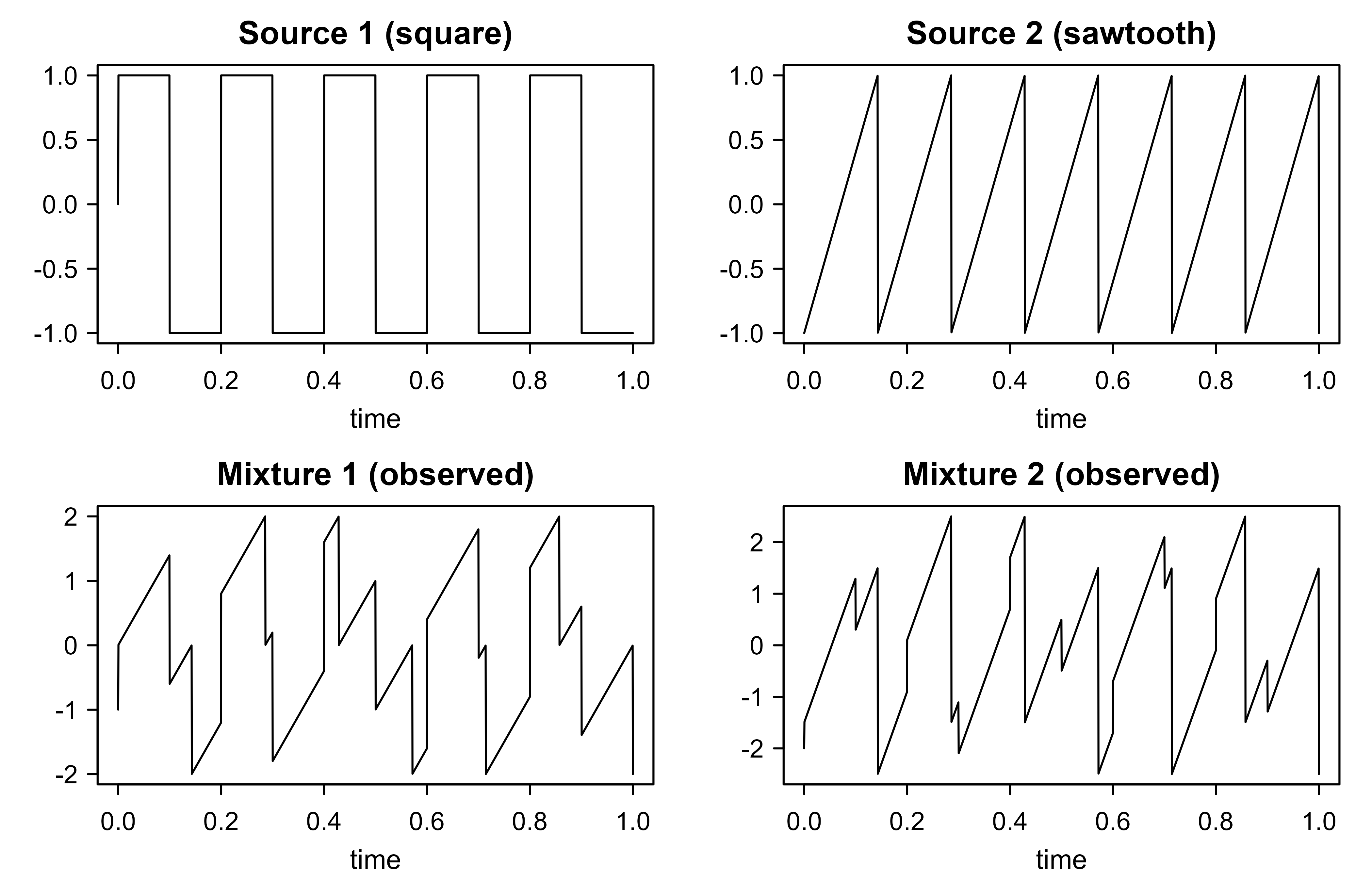
We generate two non-Gaussian sources, a square wave and a sawtooth, mix them linearly, and recover them with a from-scratch FastICA built directly from the equations above. The square and sawtooth are deliberately sub-Gaussian, so their mixtures are visibly more bell-shaped, which is the non-Gaussianity that ICA exploits.
Show code
set.seed(1)n<-2000tt<-seq(0, 1, length.out =n)s1<-sign(sin(2*pi*5*tt))# square waves2<-2*((tt*7)%%1)-1# sawtooth in [-1, 1]S<-cbind(s1, s2)S<-scale(S, center =TRUE, scale =FALSE)# center the sourcesA<-matrix(c(1, 1, 0.5, 2), nrow =2, byrow =TRUE)# mixing matrixX<-S%*%t(A)# observed mixturesop<-par(mfrow =c(2, 2), mar =c(3, 3, 2, 1), mgp =c(1.8, 0.6, 0))plot(tt, S[, 1], type ="l", main ="Source 1 (square)", xlab ="time", ylab ="")plot(tt, S[, 2], type ="l", main ="Source 2 (sawtooth)", xlab ="time", ylab ="")plot(tt, X[, 1], type ="l", main ="Mixture 1 (observed)", xlab ="time", ylab ="")plot(tt, X[, 2], type ="l", main ="Mixture 2 (observed)", xlab ="time", ylab ="")par(op)
Figure 28.1: Two independent source signals (square wave and sawtooth) and the two linear mixtures actually observed. The mixtures interleave both sources, and neither row of the mixtures resembles a clean source.
Figure 28.1 shows the latent sources and the mixtures we actually get to see. Now we whiten and run the fixed-point iteration of Equation 28.17 with the \(\tanh\) nonlinearity, extracting both components by deflation (Equation 28.18).
Show code
# --- whitening (eq. ica-whitener) ---whiten<-function(Z){Z<-sweep(Z, 2, colMeans(Z))# centere<-eigen(cov(Z), symmetric =TRUE)# eigendecomposition of covarianceV<-e$vectors%*%diag(1/sqrt(e$values))%*%t(e$vectors)list(Zw =Z%*%V, V =V)}# --- one FastICA unit via the fixed-point update (eq. fastica-update) ---fastica_one<-function(Xw, w, others, iters=300, tol=1e-10){w<-w/sqrt(sum(w^2))for(iinseq_len(iters)){wx<-as.vector(Xw%*%w)g<-tanh(wx)# g = G'gp<-1-tanh(wx)^2# g' = G''wnew<-colMeans(Xw*g)-mean(gp)*wif(length(others))# deflation: orthogonalize (eq. gram-schmidt)for(kinseq_along(others))wnew<-wnew-sum(wnew*others[[k]])*others[[k]]wnew<-wnew/sqrt(sum(wnew^2))if(1-abs(sum(wnew*w))<tol){w<-wnew; break}w<-wnew}w}wh<-whiten(X)Xw<-wh$ZwW<-list()for(jin1:2){set.seed(10+j)W[[j]]<-fastica_one(Xw, rnorm(2), W)}Wm<-do.call(rbind, W)Shat<-Xw%*%t(Wm)# estimated sources# recovery quality: best absolute correlation with a true sourcerecov<-c(max(abs(cor(Shat[, 1], S))),max(abs(cor(Shat[, 2], S))))round(recov, 3)#> [1] 1 1
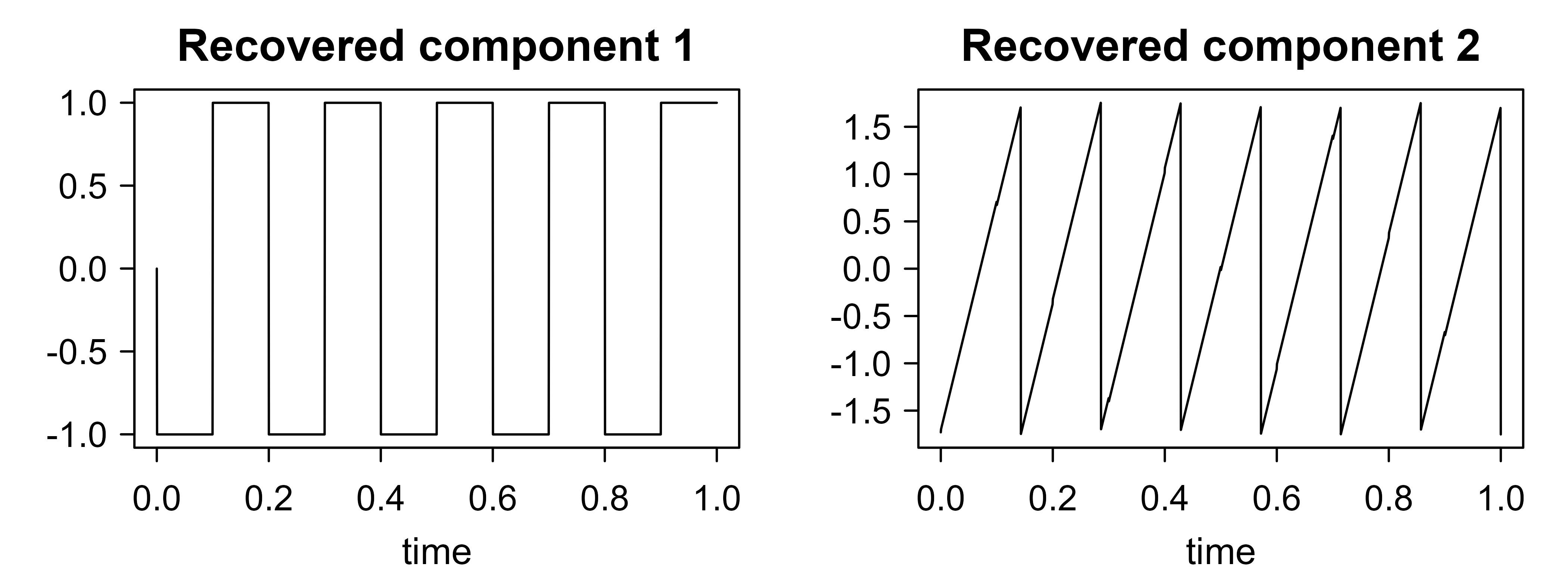
The recovered components match the true sources almost perfectly (absolute correlations near one), confirming that the fixed point of Equation 28.17 has separated the mixtures. Figure 28.2 plots them.
Show code
op<-par(mfrow =c(1, 2), mar =c(3, 3, 2, 1), mgp =c(1.8, 0.6, 0))plot(tt, Shat[, 1], type ="l", main ="Recovered component 1", xlab ="time", ylab ="")plot(tt, Shat[, 2], type ="l", main ="Recovered component 2", xlab ="time", ylab ="")par(op)
Figure 28.2: Sources recovered by the from-scratch FastICA. Up to an arbitrary sign and ordering (the two unavoidable ICA ambiguities), the square wave and sawtooth are cleanly separated from the mixtures.
For everyday use the fastICA package wraps the whitening, the symmetric fixed point, and component extraction into one call. The following reproduces the separation in a single line (it uses the same algorithm we built by hand).
Show code
# install.packages("fastICA")library(fastICA)fit<-fastICA(X, n.comp =2, fun ="logcosh", method ="C")Shat<-fit$S# estimated independent components, one per column
The contrast between this chapter and Chapter 27 is the whole lesson in miniature: PCA would have whitened these mixtures and stopped, leaving two uncorrelated but still mixed signals; ICA found the extra rotation that the non-Gaussianity of the sources made identifiable, and so pulled the voices apart.
Source Code
# Independent Component Analysis {#sec-ica}```{r}#| include: falsesource("_common.R")```Imagine standing in a crowded room where several people speak at once. Two microphones placed in different corners each pick up a different blend of all the voices. From those two mixed recordings, can you reconstruct what each individual speaker said? Your ear does something like this effortlessly, which is why the problem is known as the cocktail-party problem. Independent component analysis (ICA) is the statistical machinery that solves it without knowing anything about the voices or the room: it takes the mixed signals and pulls them back apart into the underlying sources.This is a deceptively hard task. We never observe the original voices, and we do not know how they were combined. We only see the mixtures. The remarkable claim of ICA is that, under one structural assumption (the sources are statistically independent and at most one of them is Gaussian), the unmixing can be recovered up to harmless ambiguities of scale and ordering. The single idea that makes this possible is that mixing makes signals look more Gaussian, so undoing the mixing amounts to searching for directions in which the data look as non-Gaussian as possible.ICA belongs to the same family of unsupervised, linear factorizations as principal components analysis (see @sec-dimension-reduction), and it is often introduced right after it. The two methods look superficially similar (both write the data as linear combinations of latent variables), but they optimize fundamentally different criteria. PCA seeks directions that are uncorrelated and capture maximal variance; ICA seeks directions that are statistically independent. As we will see, independence is a much stronger requirement than uncorrelatedness, and it is exactly what lets ICA separate sources that PCA cannot.::: {.callout-important title="Key idea"}PCA decorrelates (removes second-order, linear dependence) and orders directions by variance. ICA goes further and makes the recovered components statistically independent, which requires using information beyond the covariance matrix, namely the non-Gaussian structure of the data.:::## The Mixing Model {#sec-ica-model}Let there be $m$ unobserved source signals collected into a random vector $\mathbf{s} = (s_1, \dots, s_m)^\top$. We observe $m$ mixtures $\mathbf{x} = (x_1, \dots, x_m)^\top$, each a linear combination of the sources. In matrix form the generative model is$$\mathbf{x} = \mathbf{A}\,\mathbf{s},$$ {#eq-ica-mixing}where $\mathbf{A}$ is an unknown invertible $m \times m$ mixing matrix. In the cocktail-party picture, $s_j$ is the $j$th speaker, $x_i$ is the $i$th microphone, and $A_{ij}$ encodes how loudly speaker $j$ reaches microphone $i$. Given a sample of $n$ observed vectors, stacked as the rows of an $n \times m$ matrix $\mathbf{X}$, the goal is to estimate an unmixing matrix $\mathbf{W} \approx \mathbf{A}^{-1}$ so that$$\hat{\mathbf{s}} = \mathbf{W}\,\mathbf{x}$$ {#eq-ica-unmixing}recovers the sources. The defining modelling assumption is that the components of $\mathbf{s}$ are mutually statistically independent,$$p_{\mathbf{s}}(s_1, \dots, s_m) = \prod_{j=1}^m p_j(s_j),$$ {#eq-ica-indep}and that at most one of the $p_j$ is Gaussian. We also assume the sources have zero mean (we can always center the data) and, without loss of generality, unit variance, because any scaling of a source can be absorbed into the corresponding column of $\mathbf{A}$.::: {.callout-note title="The two unavoidable ambiguities"}ICA can never recover the *scale* or the *order* of the sources. If $\mathbf{P}$ is a permutation matrix and $\mathbf{D}$ a nonzero diagonal matrix, then $\mathbf{A}\mathbf{D}^{-1}\mathbf{P}^{-1}$ mixing the rescaled, reordered sources $\mathbf{P}\mathbf{D}\mathbf{s}$ produces exactly the same observations $\mathbf{x}$. We fix scale by setting unit variance and accept that the labelling and the sign of each component are arbitrary. Everything else is identifiable.:::### Why independence and non-Gaussianity identify the sources {#sec-ica-identifiability}The single deepest fact in ICA is that Gaussian sources cannot be separated, while non-Gaussian ones can. Understanding why explains the whole method.Suppose the sources are jointly Gaussian, independent, with unit variance, so $\mathbf{s} \sim \mathcal{N}(\mathbf{0}, \mathbf{I})$. Then $\mathbf{x} = \mathbf{A}\mathbf{s} \sim \mathcal{N}(\mathbf{0}, \mathbf{A}\mathbf{A}^\top)$. Now take any orthogonal matrix $\mathbf{Q}$ (so $\mathbf{Q}\mathbf{Q}^\top = \mathbf{I}$) and define a rotated set of sources $\mathbf{s}' = \mathbf{Q}\mathbf{s}$. Because the standard Gaussian is rotationally symmetric, $\mathbf{s}'$ is *also* $\mathcal{N}(\mathbf{0}, \mathbf{I})$ with independent components, and the alternative mixing matrix $\mathbf{A}' = \mathbf{A}\mathbf{Q}^\top$ gives$$\mathbf{A}'\mathbf{s}' = \mathbf{A}\mathbf{Q}^\top \mathbf{Q}\,\mathbf{s} = \mathbf{A}\mathbf{s} = \mathbf{x}.$$ {#eq-ica-gauss-rotation}The pair $(\mathbf{A}', \mathbf{s}')$ explains the data exactly as well as $(\mathbf{A}, \mathbf{s})$, and the two are not related by mere permutation and scaling. The model is unidentifiable: any rotation of jointly Gaussian sources is again valid independent Gaussian sources. Second-order statistics (the covariance) are all a Gaussian has, and the covariance is invariant to rotation, so there is simply no information left to pin down the rotation.Non-Gaussian sources break this symmetry. To see how, consider any linear combination of the observed mixtures, $y = \mathbf{w}^\top \mathbf{x} = \mathbf{w}^\top \mathbf{A}\,\mathbf{s} = \mathbf{z}^\top \mathbf{s}$, where $\mathbf{z} = \mathbf{A}^\top \mathbf{w}$. So every candidate unmixing direction $\mathbf{w}$ produces an output $y$ that is a weighted sum of the independent sources, $y = \sum_j z_j s_j$. The classical central limit theorem says that sums of independent random variables tend toward a Gaussian. Therefore a generic mixture $\sum_j z_j s_j$ is *more Gaussian* than any single source. The output $y$ is least Gaussian precisely when the sum collapses onto a single source, that is, when $\mathbf{z}$ has exactly one nonzero entry. At that point $y$ equals one of the original $s_j$ (up to scale). This gives a constructive recipe:> To recover a source, search over directions $\mathbf{w}$ for the one that makes $y = \mathbf{w}^\top \mathbf{x}$ as far from Gaussian as possible.Maximizing non-Gaussianity is the engine of ICA. Everything that follows is about how to measure "non-Gaussianity" with a tractable contrast function and how to optimize it efficiently.## Whitening: Reducing the Problem to a Rotation {#sec-ica-whitening}Before searching for the unmixing directions, it pays to preprocess the data so that the remaining work is as simple as possible. The preprocessing is whitening (also called sphering), and it is essentially the same linear-algebra step that powers PCA.Center the observed data and compute the sample covariance $\mathbf{C} = \mathbb{E}[\mathbf{x}\mathbf{x}^\top]$. Diagonalize it with its eigendecomposition $\mathbf{C} = \mathbf{E}\,\boldsymbol{\Lambda}\,\mathbf{E}^\top$, where $\mathbf{E}$ holds the orthonormal eigenvectors and $\boldsymbol{\Lambda} = \operatorname{diag}(\lambda_1, \dots, \lambda_m)$ the eigenvalues. Define the whitening matrix$$\mathbf{V} = \mathbf{E}\,\boldsymbol{\Lambda}^{-1/2}\,\mathbf{E}^\top,$$ {#eq-ica-whitener}and the whitened data $\tilde{\mathbf{x}} = \mathbf{V}\mathbf{x}$. By construction $\tilde{\mathbf{x}}$ has identity covariance:$$\mathbb{E}[\tilde{\mathbf{x}}\tilde{\mathbf{x}}^\top]= \mathbf{V}\,\mathbf{C}\,\mathbf{V}^\top= \mathbf{E}\boldsymbol{\Lambda}^{-1/2}\mathbf{E}^\top \mathbf{E}\boldsymbol{\Lambda}\mathbf{E}^\top \mathbf{E}\boldsymbol{\Lambda}^{-1/2}\mathbf{E}^\top= \mathbf{I}.$$ {#eq-ica-white-cov}Whitening removes all linear correlation and equalizes variance, which is exactly the second-order, PCA-level structure. What it cannot do is achieve independence, because that involves higher-order statistics. The crucial payoff is that, after whitening, the remaining mixing is a pure rotation. Writing $\tilde{\mathbf{x}} = \mathbf{V}\mathbf{A}\,\mathbf{s} = \tilde{\mathbf{A}}\,\mathbf{s}$ and using that $\mathbf{s}$ has identity covariance,$$\mathbf{I} = \mathbb{E}[\tilde{\mathbf{x}}\tilde{\mathbf{x}}^\top]= \tilde{\mathbf{A}}\,\mathbb{E}[\mathbf{s}\mathbf{s}^\top]\,\tilde{\mathbf{A}}^\top= \tilde{\mathbf{A}}\tilde{\mathbf{A}}^\top,$$ {#eq-ica-orthogonal}so $\tilde{\mathbf{A}}$ is orthogonal. The full unmixing problem ($m^2$ unknowns) has been reduced to finding an orthogonal matrix ($m(m-1)/2$ free parameters), which is just the search for the rotation that the identifiability argument said Gaussian data could never reveal but non-Gaussian data can. This is why ICA pipelines always whiten first: it halves the work and lets the contrast-function search operate on an orthonormal frame.::: {.callout-tip title="Mental model"}Whitening turns an arbitrary elliptical cloud into a spherical one. For Gaussian data the sphere looks the same from every angle, which is exactly why no rotation is special. For non-Gaussian data the sphere has lumpy, non-uniform structure, and ICA rotates the axes to line up with the lumps.:::## Measuring Non-Gaussianity: Contrast Functions {#sec-ica-contrast}To turn "as non-Gaussian as possible" into an objective we can optimize, we need a scalar measure of how far a (zero-mean, unit-variance) random variable $y$ is from Gaussian. Two classical choices are kurtosis and negentropy.### Kurtosis {#sec-ica-kurtosis}The (excess) kurtosis of a zero-mean variable is$$\operatorname{kurt}(y) = \mathbb{E}[y^4] - 3\big(\mathbb{E}[y^2]\big)^2.$$ {#eq-ica-kurtosis}For a Gaussian, $\mathbb{E}[y^4] = 3(\mathbb{E}[y^2])^2$, so kurtosis is exactly zero; any nonzero value signals non-Gaussianity. Distributions with positive kurtosis are super-Gaussian (heavy-tailed, spiky, like speech or a Laplace density), while negative kurtosis indicates sub-Gaussian variables (flat-topped, like a uniform distribution or many digital signals). Kurtosis is attractive because it is simple and, for unit-variance variables, behaves nicely under linear combination: if $y = \sum_j z_j s_j$ with independent $s_j$ and $\sum_j z_j^2 = 1$, then$$\operatorname{kurt}(y) = \sum_{j=1}^m z_j^4 \,\operatorname{kurt}(s_j).$$ {#eq-ica-kurt-additive}Maximizing $|\operatorname{kurt}(y)|$ over the unit sphere $\sum_j z_j^2 = 1$ drives the weight onto a single coordinate (since the quartic $\sum z_j^4$ is maximized at a vertex), exactly recovering one source. The drawback is statistical: kurtosis depends on fourth moments and is therefore extremely sensitive to outliers, which can dominate the estimate. For this reason practitioners usually prefer negentropy with a robust nonlinearity.### Negentropy {#sec-ica-negentropy}Information theory offers the principled measure. Among all distributions with a fixed variance, the Gaussian has the largest differential entropy. So the *entropy gap* between $y$ and a Gaussian of the same variance is a natural, always-nonnegative measure of non-Gaussianity. This is negentropy:$$J(y) = H(y_{\text{gauss}}) - H(y),\qquad H(y) = -\!\int p(u)\log p(u)\,du,$$ {#eq-ica-negentropy}where $y_{\text{gauss}}$ is Gaussian with the same variance as $y$. Negentropy is zero if and only if $y$ is Gaussian and positive otherwise, and unlike kurtosis it uses the entire distribution rather than a single moment, making it statistically well behaved. Its weakness is that it requires the unknown density $p$. The practical fix, due to Hyvarinen, is the approximation$$J(y) \approx \kappa \big(\mathbb{E}[G(y)] - \mathbb{E}[G(\nu)]\big)^2,$$ {#eq-ica-negentropy-approx}where $\nu \sim \mathcal{N}(0,1)$, $\kappa > 0$ is a constant, and $G$ is a smooth, slowly growing nonquadratic function. Common choices are $G(u) = \tfrac{1}{a}\log\cosh(au)$ (so $g = G' = \tanh(au)$) and $G(u) = -e^{-u^2/2}$. These robust contrasts recover the spirit of kurtosis (the special case $G(u) = u^4$) while taming the sensitivity to tails, and they lead directly to the FastICA update.## The FastICA Fixed-Point Algorithm {#sec-ica-fastica}FastICA finds, on whitened data, a unit vector $\mathbf{w}$ that maximizes the negentropy approximation in @eq-ica-negentropy-approx. We derive its update rule, which is the centerpiece of practical ICA.### Derivation of the fixed point {#sec-ica-fastica-derivation}Work with whitened data $\tilde{\mathbf{x}}$ and write $y = \mathbf{w}^\top \tilde{\mathbf{x}}$. Maximizing the approximation in @eq-ica-negentropy-approx with respect to $\mathbf{w}$ is, up to constants and sign, the same as finding the stationary points of $\mathbb{E}[G(\mathbf{w}^\top \tilde{\mathbf{x}})]$ subject to the unit-norm constraint $\|\mathbf{w}\|^2 = 1$ (the constraint preserves unit variance because the data are whitened). Form the Lagrangian$$\mathcal{L}(\mathbf{w}, \beta) = \mathbb{E}\!\left[G(\mathbf{w}^\top \tilde{\mathbf{x}})\right] - \tfrac{\beta}{2}\big(\|\mathbf{w}\|^2 - 1\big).$$ {#eq-ica-lagrangian}Setting the gradient to zero, and writing $g = G'$, gives the stationarity condition$$\mathbb{E}\!\left[\tilde{\mathbf{x}}\, g(\mathbf{w}^\top \tilde{\mathbf{x}})\right] - \beta\,\mathbf{w} = \mathbf{0}.$$ {#eq-ica-stationarity}Denote the left side by $F(\mathbf{w})$. We solve $F(\mathbf{w}) = \mathbf{0}$ with Newton's method, which needs the Jacobian. Differentiating,$$\frac{\partial F}{\partial \mathbf{w}}= \mathbb{E}\!\left[\tilde{\mathbf{x}}\tilde{\mathbf{x}}^\top g'(\mathbf{w}^\top \tilde{\mathbf{x}})\right] - \beta\,\mathbf{I}.$$ {#eq-ica-jacobian}Here comes the key approximation that gives FastICA its speed. Because the data are whitened, $\mathbb{E}[\tilde{\mathbf{x}}\tilde{\mathbf{x}}^\top] = \mathbf{I}$, so we approximate the first term by factoring the expectation:$$\mathbb{E}\!\left[\tilde{\mathbf{x}}\tilde{\mathbf{x}}^\top g'(\mathbf{w}^\top \tilde{\mathbf{x}})\right]\approx \mathbb{E}\!\left[\tilde{\mathbf{x}}\tilde{\mathbf{x}}^\top\right]\,\mathbb{E}\!\left[g'(\mathbf{w}^\top \tilde{\mathbf{x}})\right]= \mathbb{E}\!\left[g'(\mathbf{w}^\top \tilde{\mathbf{x}})\right]\mathbf{I}.$$ {#eq-ica-jac-approx}The Jacobian becomes diagonal, $\big(\mathbb{E}[g'(\mathbf{w}^\top \tilde{\mathbf{x}})] - \beta\big)\mathbf{I}$, so its inverse is trivial. The Newton step $\mathbf{w} \leftarrow \mathbf{w} - (\partial F/\partial \mathbf{w})^{-1} F(\mathbf{w})$ reads$$\mathbf{w} \leftarrow \mathbf{w} - \frac{\mathbb{E}[\tilde{\mathbf{x}}\,g(\mathbf{w}^\top \tilde{\mathbf{x}})] - \beta\,\mathbf{w}}{\mathbb{E}[g'(\mathbf{w}^\top \tilde{\mathbf{x}})] - \beta}.$$ {#eq-ica-newton}Multiplying through by the scalar $\beta - \mathbb{E}[g'(\mathbf{w}^\top \tilde{\mathbf{x}})]$ (which only rescales $\mathbf{w}$, and we renormalize anyway) collapses this into the celebrated FastICA fixed-point update$$\mathbf{w}^{+} = \mathbb{E}\!\left[\tilde{\mathbf{x}}\, g(\mathbf{w}^\top \tilde{\mathbf{x}})\right] - \mathbb{E}\!\left[g'(\mathbf{w}^\top \tilde{\mathbf{x}})\right]\mathbf{w},\qquad\mathbf{w} \leftarrow \frac{\mathbf{w}^{+}}{\|\mathbf{w}^{+}\|}.$$ {#eq-ica-fastica-update}Each iteration evaluates a nonlinearity and two sample averages, then renormalizes; there is no step size to tune, and convergence is cubic near a solution, which is why the method is fast. With $g(u) = \tanh(au)$ we have $g'(u) = a\big(1 - \tanh^2(au)\big)$, the workhorse choice.### Extracting all components {#sec-ica-deflation}A single run of @eq-ica-fastica-update finds one independent component. To get them all, two schemes are used. In *deflation* (Gram-Schmidt) we extract components one at a time and, after each update, project out the directions already found,$$\mathbf{w}_p \leftarrow \mathbf{w}_p - \sum_{j=1}^{p-1} (\mathbf{w}_p^\top \mathbf{w}_j)\,\mathbf{w}_j,\qquad\mathbf{w}_p \leftarrow \frac{\mathbf{w}_p}{\|\mathbf{w}_p\|},$$ {#eq-ica-gram-schmidt}so the new direction stays orthogonal to all previous ones (orthogonality in the whitened space is exactly the independence-preserving constraint from @eq-ica-orthogonal). In the *symmetric* scheme all rows of $\mathbf{W}$ are updated in parallel and then jointly orthogonalized via $\mathbf{W} \leftarrow (\mathbf{W}\mathbf{W}^\top)^{-1/2}\mathbf{W}$, which avoids the accumulation of error that deflation can suffer in the later components. The final unmixing matrix on the original data is $\hat{\mathbf{W}} = \mathbf{W}_{\text{white}}\,\mathbf{V}$, combining the learned rotation with the whitener of @eq-ica-whitener.## ICA Versus PCA {#sec-ica-vs-pca}It is worth stating the contrast with @sec-dimension-reduction sharply, because the two methods are so often confused.| Aspect | PCA | ICA ||---|---|---|| Criterion | maximal variance | maximal independence (non-Gaussianity) || Statistics used | second order (covariance) | higher order (kurtosis, negentropy) || Output relation | uncorrelated, orthogonal | independent, generally non-orthogonal in data space || Ordering | by variance (meaningful) | none (arbitrary sign and order) || Goal | compression, denoising | source separation, latent structure |: PCA and ICA optimize different things. {#tbl-ica-pca}@tbl-ica-pca makes the central point: uncorrelated is not the same as independent. Independence implies uncorrelatedness, but the converse holds only for Gaussian variables. PCA stops at the covariance and therefore at uncorrelatedness; ICA exploits the non-Gaussian higher-order structure to reach full independence. A useful summary is that PCA does the whitening step of ICA (@sec-ica-whitening) and then stops, whereas ICA additionally finds the special rotation of the whitened data that lines the axes up with the independent sources. PCA is the right tool when the goal is to capture variance and compress; ICA is the right tool when the goal is to recover physically meaningful, independent generative factors.## Assumptions, Properties, and Failure Modes {#sec-ica-properties}A careful user should keep the following in mind.- **Independence and non-Gaussianity are load-bearing.** If two or more sources are Gaussian, those sources occupy a subspace that ICA can identify but cannot resolve internally (the rotation within it is free, by @eq-ica-gauss-rotation). At most one Gaussian source is allowed.- **Sign, scale, and order are unidentifiable.** A recovered component can be flipped, rescaled, or relabelled relative to the true source. Downstream interpretation must account for this.- **Square, noiseless model by default.** The basic model assumes as many mixtures as sources ($\mathbf{A}$ square and invertible) and no additive noise. Overcomplete ICA (more sources than sensors) and noisy ICA require richer estimators and are genuinely harder.- **Complexity.** Whitening costs $O(nm^2 + m^3)$. Each FastICA iteration over $m$ components is $O(nm^2)$, and the fixed point typically converges in a handful of iterations, so ICA scales comfortably to large $n$ and moderate $m$.- **Statistical conditioning.** Kurtosis-based contrasts are fragile to outliers; the robust $\log\cosh$ contrast (@sec-ica-negentropy) is the safer default. Convergence can land on a local optimum, so multiple random restarts are good practice.- **Connections.** ICA is a maximum-likelihood method when the source densities are specified, and it can be read as a single-layer linear generative model. This links it to nonlinear and probabilistic latent-variable models such as autoencoders (@sec-autoencoders) and deep generative models (@sec-generative-models), which relax the linearity of @eq-ica-mixing. It is also a tool for unsupervised structure discovery alongside clustering (@sec-cluster) and density estimation (@sec-density-estimation).::: {.callout-warning title="When ICA will disappoint you"}ICA assumes instantaneous linear mixing. Real audio in a room involves echoes and delays (convolutive mixing), which the basic model does not capture; convolutive ICA or time-frequency methods are needed there. ICA also gives no inherent ranking of components, so do not expect the first recovered component to be the most important one.:::## Practical How-To {#sec-ica-howto}A reliable ICA workflow looks like this.1. **Center** the data (subtract the column means) and, if features are on very different scales, consider standardizing.2. **Choose the number of components.** With noise or many sensors, first reduce dimension with PCA (@sec-dimension-reduction), keeping the leading components, then run ICA on that subspace. This both denoises and sets $m$.3. **Whiten** using @eq-ica-whitener.4. **Run FastICA** with a robust nonlinearity ($\tanh$ by default), using the symmetric orthogonalization (@sec-ica-deflation) and several random initializations.5. **Interpret with care.** Fix signs and an ordering by a convention that suits the application (for example, order by the variance the component explains in the original data, or by kurtosis), and remember these choices are arbitrary.In R the `fastICA` package implements all of this. For transparency the demonstration below also includes a from-scratch fixed-point implementation so the mechanics of @eq-ica-fastica-update are fully visible.## A Runnable Demonstration {#sec-ica-demo}We generate two non-Gaussian sources, a square wave and a sawtooth, mix them linearly, and recover them with a from-scratch FastICA built directly from the equations above. The square and sawtooth are deliberately sub-Gaussian, so their mixtures are visibly more bell-shaped, which is the non-Gaussianity that ICA exploits.```{r}#| label: fig-ica-signals#| fig-cap: "Two independent source signals (square wave and sawtooth) and the two linear mixtures actually observed. The mixtures interleave both sources, and neither row of the mixtures resembles a clean source."#| fig-width: 7#| fig-height: 4.5set.seed(1)n <-2000tt <-seq(0, 1, length.out = n)s1 <-sign(sin(2* pi *5* tt)) # square waves2 <-2* ((tt *7) %%1) -1# sawtooth in [-1, 1]S <-cbind(s1, s2)S <-scale(S, center =TRUE, scale =FALSE) # center the sourcesA <-matrix(c(1, 1, 0.5, 2), nrow =2, byrow =TRUE) # mixing matrixX <- S %*%t(A) # observed mixturesop <-par(mfrow =c(2, 2), mar =c(3, 3, 2, 1), mgp =c(1.8, 0.6, 0))plot(tt, S[, 1], type ="l", main ="Source 1 (square)", xlab ="time", ylab ="")plot(tt, S[, 2], type ="l", main ="Source 2 (sawtooth)", xlab ="time", ylab ="")plot(tt, X[, 1], type ="l", main ="Mixture 1 (observed)", xlab ="time", ylab ="")plot(tt, X[, 2], type ="l", main ="Mixture 2 (observed)", xlab ="time", ylab ="")par(op)```@fig-ica-signals shows the latent sources and the mixtures we actually get to see. Now we whiten and run the fixed-point iteration of @eq-ica-fastica-update with the $\tanh$ nonlinearity, extracting both components by deflation (@eq-ica-gram-schmidt).```{r}#| label: ica-fit# --- whitening (eq. ica-whitener) ---whiten <-function(Z) { Z <-sweep(Z, 2, colMeans(Z)) # center e <-eigen(cov(Z), symmetric =TRUE) # eigendecomposition of covariance V <- e$vectors %*%diag(1/sqrt(e$values)) %*%t(e$vectors)list(Zw = Z %*% V, V = V)}# --- one FastICA unit via the fixed-point update (eq. fastica-update) ---fastica_one <-function(Xw, w, others, iters =300, tol =1e-10) { w <- w /sqrt(sum(w^2))for (i inseq_len(iters)) { wx <-as.vector(Xw %*% w) g <-tanh(wx) # g = G' gp <-1-tanh(wx)^2# g' = G'' wnew <-colMeans(Xw * g) -mean(gp) * wif (length(others)) # deflation: orthogonalize (eq. gram-schmidt)for (k inseq_along(others)) wnew <- wnew -sum(wnew * others[[k]]) * others[[k]] wnew <- wnew /sqrt(sum(wnew^2))if (1-abs(sum(wnew * w)) < tol) { w <- wnew; break } w <- wnew } w}wh <-whiten(X)Xw <- wh$ZwW <-list()for (j in1:2) {set.seed(10+ j) W[[j]] <-fastica_one(Xw, rnorm(2), W)}Wm <-do.call(rbind, W)Shat <- Xw %*%t(Wm) # estimated sources# recovery quality: best absolute correlation with a true sourcerecov <-c(max(abs(cor(Shat[, 1], S))),max(abs(cor(Shat[, 2], S))))round(recov, 3)```The recovered components match the true sources almost perfectly (absolute correlations near one), confirming that the fixed point of @eq-ica-fastica-update has separated the mixtures. @fig-ica-recovered plots them.```{r}#| label: fig-ica-recovered#| fig-cap: "Sources recovered by the from-scratch FastICA. Up to an arbitrary sign and ordering (the two unavoidable ICA ambiguities), the square wave and sawtooth are cleanly separated from the mixtures."#| fig-width: 7#| fig-height: 2.6op <-par(mfrow =c(1, 2), mar =c(3, 3, 2, 1), mgp =c(1.8, 0.6, 0))plot(tt, Shat[, 1], type ="l", main ="Recovered component 1", xlab ="time", ylab ="")plot(tt, Shat[, 2], type ="l", main ="Recovered component 2", xlab ="time", ylab ="")par(op)```For everyday use the `fastICA` package wraps the whitening, the symmetric fixed point, and component extraction into one call. The following reproduces the separation in a single line (it uses the same algorithm we built by hand).```{r}#| label: ica-package#| eval: false# install.packages("fastICA")library(fastICA)fit <-fastICA(X, n.comp =2, fun ="logcosh", method ="C")Shat <- fit$S # estimated independent components, one per column```The contrast between this chapter and @sec-dimension-reduction is the whole lesson in miniature: PCA would have whitened these mixtures and stopped, leaving two uncorrelated but still mixed signals; ICA found the extra rotation that the non-Gaussianity of the sources made identifiable, and so pulled the voices apart.