Advanced Data Analysis

Nguyen, Mike

43 Diffusion Models

Picture a clear photograph. Now imagine sprinkling a little static onto it, then a little more, and a little more, until after a few hundred steps nothing is left but pure television snow. That destruction is easy: anyone can add noise. The hard and interesting question is whether a model can learn to run the tape backward, starting from snow and removing noise one careful step at a time until a brand new, never seen photograph emerges. A diffusion model is exactly a learned procedure for reversing noise. It is trained on the easy forward direction, where we know precisely how much noise we added, and it uses that knowledge to take small, confident steps in the hard reverse direction.

This idea now powers most state of the art image, audio, and video generators. It belongs to the family of generative models (Chapter 42) alongside variational autoencoders and generative adversarial networks, but it reaches the goal, a model you can sample from, by a route that is unusually stable to train and unusually clean to analyze. The reason is that every quantity we need has a closed form. We never have to fight an adversary the way a GAN does, and we never have to approximate an intractable posterior the way a plain VAE does. We simply teach a network to predict the noise that was added, and almost everything else follows from Gaussian algebra.

Intuition

Adding noise is a one way street that is trivial to walk forward. A diffusion model learns a guidebook for walking back up that street. Because each forward step is a tiny Gaussian nudge, each backward step is also approximately Gaussian, and predicting one small nudge at a time is far easier than inventing a whole image in one shot.

This chapter develops the model in the order that makes the math honest. We first define the forward noising process and derive its closed form marginal, which is the single fact that makes everything else tractable. We then write the reverse process as a learned Markov chain, connect its training objective to the evidence lower bound (ELBO), and show how that objective collapses into a strikingly simple noise prediction loss. From there we cover sampling (the ancestral DDPM sampler and the deterministic DDIM shortcut), the relationships to VAEs (Chapter 41) and to score based stochastic differential equations, and classifier free guidance. A runnable base R demonstration closes the chapter by forward diffusing a one dimensional distribution and verifying the closed form variance schedule numerically.

43.1 The forward process

Let $\mathbf{x}_0 \in \mathbb{R}^d$ be a data point drawn from the unknown data distribution $q(\mathbf{x}_0)$. The forward process is a fixed (not learned) Markov chain that gradually adds Gaussian noise over $T$ steps, producing latents $\mathbf{x}_1, \dots, \mathbf{x}_T$. Each step is

\[ q(\mathbf{x}_t \mid \mathbf{x}_{t-1}) = \mathcal{N}\!\big(\mathbf{x}_t;\ \sqrt{1-\beta_t}\,\mathbf{x}_{t-1},\ \beta_t \mathbf{I}\big), \tag{43.1}\]

where the variances $\beta_1, \dots, \beta_T \in (0,1)$ form a fixed schedule that usually increases with $t$. The factor $\sqrt{1-\beta_t}$ in the mean shrinks the previous state slightly while $\beta_t \mathbf{I}$ injects fresh noise; this particular pairing is what keeps the total variance from exploding, as we verify below. The full forward chain factorizes as

\[ q(\mathbf{x}_{1:T} \mid \mathbf{x}_0) = \prod_{t=1}^{T} q(\mathbf{x}_t \mid \mathbf{x}_{t-1}). \tag{43.2}\]

If $T$ is large and the schedule is chosen so that $\prod_t (1-\beta_t)$ becomes tiny, then $q(\mathbf{x}_T)$ is essentially a standard normal $\mathcal{N}(\mathbf{0}, \mathbf{I})$ regardless of where $\mathbf{x}_0$ started. That terminal distribution is what we will sample from at generation time, so it must be something we can sample trivially, and the standard normal is.

Key idea

The forward process has no parameters to learn. It is a known corruption recipe. All of the learning happens in the reverse process, whose only job is to undo this recipe one step at a time.

43.1.1 The closed form marginal

The chain in Equation 43.2 looks like it requires $t$ sequential samples to reach $\mathbf{x}_t$. It does not. Because the composition of Gaussians is Gaussian, we can jump from $\mathbf{x}_0$ to any $\mathbf{x}_t$ in a single step. Define

\[ \alpha_t = 1 - \beta_t, \qquad \bar{\alpha}_t = \prod_{s=1}^{t} \alpha_s . \tag{43.3}\]

The claim is the marginal

\[ q(\mathbf{x}_t \mid \mathbf{x}_0) = \mathcal{N}\!\big(\mathbf{x}_t;\ \sqrt{\bar{\alpha}_t}\,\mathbf{x}_0,\ (1-\bar{\alpha}_t)\mathbf{I}\big). \tag{43.4}\]

This is the workhorse of the whole theory. Let us derive it.

Using the reparameterization trick, Equation 43.1 says

\[ \mathbf{x}_t = \sqrt{\alpha_t}\,\mathbf{x}_{t-1} + \sqrt{1-\alpha_t}\,\boldsymbol{\epsilon}_{t-1}, \qquad \boldsymbol{\epsilon}_{t-1} \sim \mathcal{N}(\mathbf{0}, \mathbf{I}), \]

and the noise variables at different steps are independent. Substitute one step into the next:

\[ \begin{aligned} \mathbf{x}_t &= \sqrt{\alpha_t}\big(\sqrt{\alpha_{t-1}}\,\mathbf{x}_{t-2} + \sqrt{1-\alpha_{t-1}}\,\boldsymbol{\epsilon}_{t-2}\big) + \sqrt{1-\alpha_t}\,\boldsymbol{\epsilon}_{t-1} \\ &= \sqrt{\alpha_t \alpha_{t-1}}\,\mathbf{x}_{t-2} + \underbrace{\sqrt{\alpha_t(1-\alpha_{t-1})}\,\boldsymbol{\epsilon}_{t-2} + \sqrt{1-\alpha_t}\,\boldsymbol{\epsilon}_{t-1}}_{\text{sum of two independent Gaussians}}. \end{aligned} \]

The bracketed term is a sum of two independent zero mean Gaussians, so it is itself zero mean Gaussian with variance equal to the sum of the variances,

\[ \alpha_t(1-\alpha_{t-1}) + (1-\alpha_t) = 1 - \alpha_t \alpha_{t-1}. \]

Therefore $\mathbf{x}_t = \sqrt{\alpha_t \alpha_{t-1}}\,\mathbf{x}_{t-2} + \sqrt{1-\alpha_t\alpha_{t-1}}\,\bar{\boldsymbol{\epsilon}}$ with $\bar{\boldsymbol{\epsilon}} \sim \mathcal{N}(\mathbf{0},\mathbf{I})$. Iterating this collapse all the way down to $\mathbf{x}_0$ replaces the product $\alpha_t \alpha_{t-1} \cdots$ with $\bar{\alpha}_t$, giving

\[ \mathbf{x}_t = \sqrt{\bar{\alpha}_t}\,\mathbf{x}_0 + \sqrt{1-\bar{\alpha}_t}\,\boldsymbol{\epsilon}, \qquad \boldsymbol{\epsilon} \sim \mathcal{N}(\mathbf{0}, \mathbf{I}), \tag{43.5}\]

which is precisely Equation 43.4 in sampled form. Two consequences are immediate. First, the signal coefficient $\sqrt{\bar{\alpha}_t}$ and the noise coefficient $\sqrt{1-\bar{\alpha}_t}$ always satisfy $\bar{\alpha}_t + (1-\bar{\alpha}_t) = 1$, so the marginal variance of any coordinate stays bounded as $t$ grows (this is the variance preserving property we verify numerically later). Second, training never needs the intermediate latents: to get a training pair at any timestep $t$ we draw one $\boldsymbol{\epsilon}$ and apply Equation 43.5 directly.

Note

The clean separation in Equation 43.5, a deterministic scaling of the data plus a single Gaussian noise vector, is the reason diffusion training is cheap. We can sample any noise level $t$ in $O(1)$ work rather than simulating $t$ chained steps.

43.1.2 The forward posterior is Gaussian

To build a reverse model we need to know, conditioned on the original $\mathbf{x}_0$, what the previous state $\mathbf{x}_{t-1}$ looked like given $\mathbf{x}_t$. This forward posterior $q(\mathbf{x}_{t-1} \mid \mathbf{x}_t, \mathbf{x}_0)$ is tractable and Gaussian. By Bayes rule within the chain,

\[ q(\mathbf{x}_{t-1} \mid \mathbf{x}_t, \mathbf{x}_0) = \mathcal{N}\!\big(\mathbf{x}_{t-1};\ \tilde{\boldsymbol{\mu}}_t(\mathbf{x}_t, \mathbf{x}_0),\ \tilde{\beta}_t \mathbf{I}\big), \tag{43.6}\]

with

\[ \tilde{\boldsymbol{\mu}}_t = \frac{\sqrt{\bar{\alpha}_{t-1}}\,\beta_t}{1-\bar{\alpha}_t}\,\mathbf{x}_0 + \frac{\sqrt{\alpha_t}\,(1-\bar{\alpha}_{t-1})}{1-\bar{\alpha}_t}\,\mathbf{x}_t, \qquad \tilde{\beta}_t = \frac{1-\bar{\alpha}_{t-1}}{1-\bar{\alpha}_t}\,\beta_t . \tag{43.7}\]

These follow from multiplying the two Gaussians $q(\mathbf{x}_t\mid\mathbf{x}_{t-1})$ and $q(\mathbf{x}_{t-1}\mid\mathbf{x}_0)$ and completing the square in $\mathbf{x}_{t-1}$; the algebra is the standard Gaussian product identity, and the resulting mean is a precision weighted average of the two contributing means. The point of Equation 43.6 is that the true reverse step, when we are allowed to peek at $\mathbf{x}_0$, is exactly Gaussian. The job of the network will be to match this Gaussian without peeking.

43.2 The reverse process and the ELBO

At generation time we do not know $\mathbf{x}_0$, so we approximate the reverse step with a learned Gaussian whose mean is a neural network $\boldsymbol{\mu}_\theta$ and whose covariance is fixed (or also learned),

\[ p_\theta(\mathbf{x}_{t-1} \mid \mathbf{x}_t) = \mathcal{N}\!\big(\mathbf{x}_{t-1};\ \boldsymbol{\mu}_\theta(\mathbf{x}_t, t),\ \sigma_t^2 \mathbf{I}\big), \tag{43.8}\]

starting from $p(\mathbf{x}_T) = \mathcal{N}(\mathbf{0}, \mathbf{I})$ and running $t = T, T-1, \dots, 1$. The generative model is the marginal $p_\theta(\mathbf{x}_0) = \int p(\mathbf{x}_T)\prod_t p_\theta(\mathbf{x}_{t-1}\mid\mathbf{x}_t)\, d\mathbf{x}_{1:T}$.

This is structurally a hierarchical VAE with $T$ stochastic layers, a fixed encoder (the forward process), and a learned decoder (the reverse process). As in any latent variable model, the marginal likelihood is intractable, so we maximize a variational lower bound. The same Jensen inequality used for the VAE in Chapter 41 gives the ELBO

\[ \log p_\theta(\mathbf{x}_0) \ \ge\ \mathbb{E}_q\!\left[\log \frac{p_\theta(\mathbf{x}_{0:T})}{q(\mathbf{x}_{1:T}\mid\mathbf{x}_0)}\right] =: -\mathcal{L}. \tag{43.9}\]

The negative ELBO $\mathcal{L}$ is what we minimize. Because both numerator and denominator factorize over $t$, $\mathcal{L}$ decomposes into per step terms. After regrouping (the standard Sohl-Dickstein/Ho derivation), the bound becomes a sum of KL divergences between Gaussians:

\[ \mathcal{L} = \underbrace{D_{\mathrm{KL}}\!\big(q(\mathbf{x}_T\mid\mathbf{x}_0)\,\|\,p(\mathbf{x}_T)\big)}_{L_T} + \sum_{t=2}^{T}\underbrace{\mathbb{E}_q\, D_{\mathrm{KL}}\!\big(q(\mathbf{x}_{t-1}\mid\mathbf{x}_t,\mathbf{x}_0)\,\|\,p_\theta(\mathbf{x}_{t-1}\mid\mathbf{x}_t)\big)}_{L_{t-1}} - \underbrace{\mathbb{E}_q \log p_\theta(\mathbf{x}_0\mid\mathbf{x}_1)}_{L_0}. \tag{43.10}\]

The first term $L_T$ has no parameters: it measures how close the fully noised data is to the standard normal prior, and with a well chosen schedule it is negligible. The reconstruction term $L_0$ handles the final decode to data space. The interesting work is in the middle terms $L_{t-1}$, each of which is a KL between two Gaussians: the tractable forward posterior Equation 43.6 and the learned reverse step Equation 43.8.

43.2.1 From KL divergence to noise prediction

For two Gaussians with the same covariance $\sigma_t^2 \mathbf{I}$, the KL divergence reduces to a scaled squared distance between their means,

\[ L_{t-1} = \mathbb{E}_q\!\left[\frac{1}{2\sigma_t^2}\,\big\|\tilde{\boldsymbol{\mu}}_t(\mathbf{x}_t,\mathbf{x}_0) - \boldsymbol{\mu}_\theta(\mathbf{x}_t, t)\big\|^2\right] + \text{const}. \tag{43.11}\]

So the network’s mean $\boldsymbol{\mu}_\theta$ should match the posterior mean $\tilde{\boldsymbol{\mu}}_t$. Here is the elegant simplification. Solve Equation 43.5 for $\mathbf{x}_0 = (\mathbf{x}_t - \sqrt{1-\bar{\alpha}_t}\,\boldsymbol{\epsilon})/\sqrt{\bar{\alpha}_t}$ and substitute into $\tilde{\boldsymbol{\mu}}_t$ from Equation 43.7. After simplification the posterior mean depends on $\mathbf{x}_t$ and the noise $\boldsymbol{\epsilon}$ only:

\[ \tilde{\boldsymbol{\mu}}_t = \frac{1}{\sqrt{\alpha_t}}\left(\mathbf{x}_t - \frac{\beta_t}{\sqrt{1-\bar{\alpha}_t}}\,\boldsymbol{\epsilon}\right). \tag{43.12}\]

This suggests parameterizing the network not as a mean predictor but as a noise predictor $\boldsymbol{\epsilon}_\theta(\mathbf{x}_t, t)$ that guesses which $\boldsymbol{\epsilon}$ was added, and then setting

\[ \boldsymbol{\mu}_\theta(\mathbf{x}_t, t) = \frac{1}{\sqrt{\alpha_t}}\left(\mathbf{x}_t - \frac{\beta_t}{\sqrt{1-\bar{\alpha}_t}}\,\boldsymbol{\epsilon}_\theta(\mathbf{x}_t, t)\right). \tag{43.13}\]

Plugging Equation 43.12 and Equation 43.13 into Equation 43.11, the difference of means becomes a difference of noise vectors, and $L_{t-1}$ turns into

\[ L_{t-1} = \mathbb{E}_{\mathbf{x}_0, \boldsymbol{\epsilon}}\!\left[\frac{\beta_t^2}{2\sigma_t^2\,\alpha_t\,(1-\bar{\alpha}_t)}\,\big\|\boldsymbol{\epsilon} - \boldsymbol{\epsilon}_\theta(\sqrt{\bar{\alpha}_t}\mathbf{x}_0 + \sqrt{1-\bar{\alpha}_t}\boldsymbol{\epsilon},\ t)\big\|^2\right]. \tag{43.14}\]

Every term is now a weighted mean squared error between the true noise and the predicted noise. Ho, Jain, and Abbeel (2020) observed that simply dropping the awkward per step weight and using the unweighted version trains better in practice, giving the famous simplified objective

\[ \mathcal{L}_{\text{simple}} = \mathbb{E}_{t,\,\mathbf{x}_0,\,\boldsymbol{\epsilon}}\!\left[\big\|\boldsymbol{\epsilon} - \boldsymbol{\epsilon}_\theta(\sqrt{\bar{\alpha}_t}\,\mathbf{x}_0 + \sqrt{1-\bar{\alpha}_t}\,\boldsymbol{\epsilon},\ t)\big\|^2\right], \tag{43.15}\]

with $t$ drawn uniformly over $\{1, \dots, T\}$. This is just regression. The network sees a noisy input and a timestep and predicts the noise; the loss is plain squared error. There is no adversary and no sampling inside the loss, which is why diffusion training is so stable.

Key idea

The entire training procedure is: pick a random data point, pick a random timestep, add a known amount of Gaussian noise, and train a network to predict that noise with mean squared error. The ELBO derivation justifies this, but the implementation is a few lines.

43.2.2 Connection to denoising score matching

The noise prediction objective is the same thing as score matching (Chapter 32), viewed through a change of variable. The score of the noised marginal is the gradient of its log density, $\mathbf{s}(\mathbf{x}_t) = \nabla_{\mathbf{x}_t} \log q(\mathbf{x}_t)$. For the Gaussian marginal Equation 43.4, that score equals $-\boldsymbol{\epsilon}/\sqrt{1-\bar{\alpha}_t}$ in expectation, so a network that predicts $\boldsymbol{\epsilon}$ is, up to the scaling $-1/\sqrt{1-\bar{\alpha}_t}$, predicting the score. Minimizing Equation 43.15 is therefore denoising score matching across a continuum of noise levels. This is the bridge to the score based view we describe next, and it is why people use the words “score model” and “diffusion model” almost interchangeably.

43.3 Sampling

Once $\boldsymbol{\epsilon}_\theta$ is trained, generation runs the learned reverse chain. The ancestral (DDPM) sampler starts from $\mathbf{x}_T \sim \mathcal{N}(\mathbf{0}, \mathbf{I})$ and, for $t = T, \dots, 1$, draws

\[ \mathbf{x}_{t-1} = \frac{1}{\sqrt{\alpha_t}}\left(\mathbf{x}_t - \frac{\beta_t}{\sqrt{1-\bar{\alpha}_t}}\,\boldsymbol{\epsilon}_\theta(\mathbf{x}_t, t)\right) + \sigma_t\,\mathbf{z}, \qquad \mathbf{z} \sim \mathcal{N}(\mathbf{0}, \mathbf{I}), \tag{43.16}\]

with $\mathbf{z} = \mathbf{0}$ at the last step, and $\sigma_t^2$ typically set to $\beta_t$ or to the posterior variance $\tilde{\beta}_t$. The deterministic mean here is exactly Equation 43.13, and the added $\sigma_t \mathbf{z}$ is the stochastic part of the reverse step. The drawback is cost: faithful samples often need hundreds or thousands of steps, each a full network evaluation.

DDIM (Song, Meng, Ermon 2021) removes most of that cost. It defines a non Markovian forward process that shares the same marginals Equation 43.4, so the same trained $\boldsymbol{\epsilon}_\theta$ applies, but whose reverse step can be made deterministic. The DDIM update first estimates the clean signal $\hat{\mathbf{x}}_0 = (\mathbf{x}_t - \sqrt{1-\bar{\alpha}_t}\,\boldsymbol{\epsilon}_\theta)/\sqrt{\bar{\alpha}_t}$, then re-noises it to level $t-1$:

\[ \mathbf{x}_{t-1} = \sqrt{\bar{\alpha}_{t-1}}\,\hat{\mathbf{x}}_0 + \sqrt{1-\bar{\alpha}_{t-1}}\,\boldsymbol{\epsilon}_\theta(\mathbf{x}_t, t). \tag{43.17}\]

Because there is no injected noise, the map from $\mathbf{x}_T$ to $\mathbf{x}_0$ is deterministic, the same seed always gives the same image, and one can skip timesteps aggressively, generating in 10 to 50 steps instead of 1000. DDIM trades a little sample diversity for a large speedup and is the practical default for many systems.

Practical note

The DDPM sampler is stochastic and tends to give more diverse, slightly higher fidelity samples at high step counts; the DDIM sampler is deterministic and far faster at low step counts. Switching between them needs no retraining, since both use the same $\boldsymbol{\epsilon}_\theta$.

43.4 Connections: VAEs and score based SDEs

Two viewpoints unify diffusion with the rest of the book.

As a hierarchical VAE (Chapter 41), a diffusion model is a VAE whose encoder is fixed and hand designed (the noising chain) rather than learned, with $T$ latent layers instead of one. This is why the same ELBO machinery applies verbatim. The crucial difference from an ordinary VAE is that the fixed encoder has a closed form posterior Equation 43.6, so the KL terms are exact Gaussian KLs with no amortization gap and no posterior collapse.

As a stochastic differential equation, take the limit $T \to \infty$ with infinitesimal steps. The discrete forward chain becomes a continuous time SDE \[ d\mathbf{x} = -\tfrac{1}{2}\beta(t)\,\mathbf{x}\,dt + \sqrt{\beta(t)}\,d\mathbf{w}, \] where $\mathbf{w}$ is a Wiener process. Anderson’s reverse time SDE theorem says the corresponding reverse process is \[ d\mathbf{x} = \big[-\tfrac{1}{2}\beta(t)\mathbf{x} - \beta(t)\,\nabla_{\mathbf{x}}\log q_t(\mathbf{x})\big]dt + \sqrt{\beta(t)}\,d\bar{\mathbf{w}}, \] which needs only the score $\nabla_{\mathbf{x}}\log q_t$, exactly what $\boldsymbol{\epsilon}_\theta$ learns. There is also a deterministic probability flow ODE with the same marginals, which is the continuous time cousin of DDIM and connects diffusion to normalizing flows and to Gaussian process style continuous dynamics (Chapter 7). This SDE picture is what licenses the many fast ODE solvers (for example DPM-Solver) used in production.

43.5 Classifier free guidance

To steer generation with a condition $c$ (a class label or a text prompt), one trains a single conditional network $\boldsymbol{\epsilon}_\theta(\mathbf{x}_t, t, c)$ but randomly drops the condition during training (replacing $c$ with a null token) so the same weights also learn the unconditional score $\boldsymbol{\epsilon}_\theta(\mathbf{x}_t, t, \varnothing)$. At sampling time the two predictions are combined with a guidance weight $w \ge 0$, \[ \tilde{\boldsymbol{\epsilon}} = (1+w)\,\boldsymbol{\epsilon}_\theta(\mathbf{x}_t, t, c) - w\,\boldsymbol{\epsilon}_\theta(\mathbf{x}_t, t, \varnothing), \] which extrapolates away from the unconditional direction and toward the conditional one, sharpening adherence to $c$ at some cost in diversity. This classifier free scheme (Ho and Salimans 2022) avoids training a separate classifier on noisy inputs and is the standard conditioning method in modern text to image systems.

43.6 Practical considerations

A few facts matter when building or reading about these models.

Architecture. $\boldsymbol{\epsilon}_\theta$ for images is almost always a U-Net with residual blocks and self attention (Chapter 38); the timestep $t$ enters through a sinusoidal embedding added to each block. The network shares weights across all timesteps. These pieces need a GPU and a deep learning backend, so the neural code in this chapter is shown unevaluated.
Noise schedule. A linear $\beta_t$ schedule works but a cosine schedule for $\bar{\alpha}_t$ usually trains better by spending more steps at low noise. The schedule fully determines $\bar{\alpha}_t$ and hence the forward marginals.
Cost. Training is cheap per step (one forward and backward pass on a noisy image) but sampling is expensive (one network call per reverse step). DDIM and ODE solvers cut sampling steps by one to two orders of magnitude.
Failure modes. Too few sampling steps gives blurry or artifact ridden outputs; a poorly tuned schedule wastes capacity at noise levels that carry little signal; overly large guidance weights produce oversaturated, low diversity samples. Unlike GANs, diffusion models rarely suffer mode collapse, which is one of their main attractions.
Likelihoods. The ELBO gives a real (if loose) bound on log likelihood, so diffusion models can report calibrated likelihoods, something GANs cannot.

Warning

The simplified loss Equation 43.15 drops the ELBO weights, so the quantity you minimize is no longer a valid likelihood bound. It generates better samples but you should not read $\mathcal{L}_{\text{simple}}$ as a log likelihood. To report likelihoods, use the weighted variational bound Equation 43.10.

43.7 A runnable demonstration: forward diffusion in one dimension

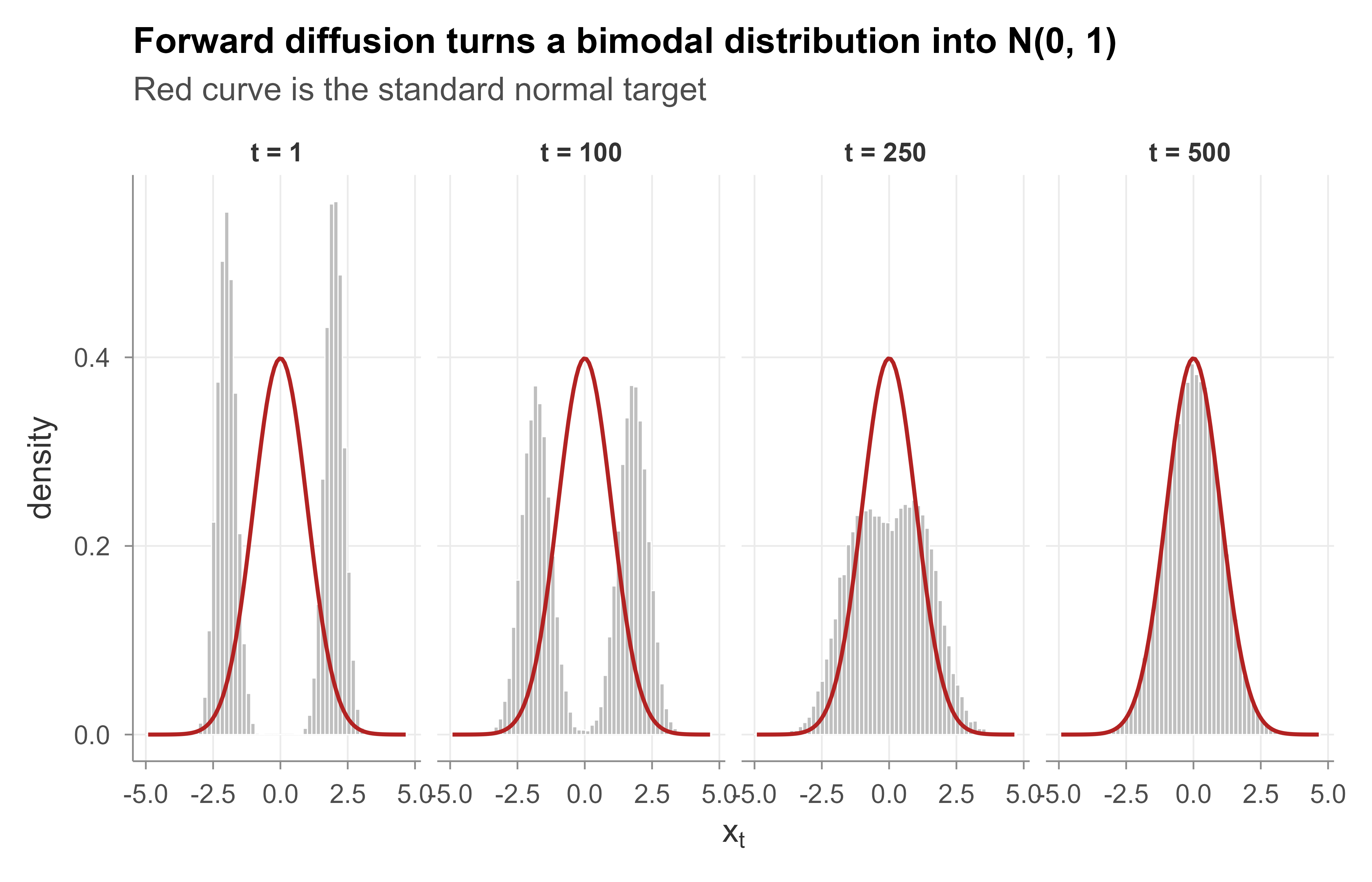
The neural reverse model needs a GPU, but the forward process and its closed form marginal are pure algebra that we can verify exactly in base R. The demonstration below takes a simple non Gaussian one dimensional distribution (a two component mixture), runs the forward chain Equation 43.1 step by step on a large sample, and checks two things: that the empirical mean and variance at each timestep match the closed form $\sqrt{\bar{\alpha}_t}\,\mathbf{x}_0$ scaling and the $1-\bar{\alpha}_t$ variance growth predicted by Equation 43.4, and that the distribution morphs from a clearly bimodal shape into a standard normal.

Show code

set.seed(1301)

## ---- A simple non-Gaussian data distribution: a two-component mixture ----
n <- 40000
comp <- rbinom(n, 1, 0.5)
x0   <- ifelse(comp == 1, rnorm(n, mean = -2.0, sd = 0.35),
                          rnorm(n, mean =  2.0, sd = 0.35))

## ---- Forward noise schedule (linear betas, the original DDPM choice) ----
TT      <- 500
beta    <- seq(1e-4, 0.02, length.out = TT)   # increasing variances
alpha   <- 1 - beta
abar    <- cumprod(alpha)                     # alpha-bar_t (eq-diffusion-alphabar)

## ---- Run the forward Markov chain step by step (no closed form used) ----
## x_t = sqrt(alpha_t) x_{t-1} + sqrt(beta_t) * noise
X <- x0
snapshots <- list()
keep <- c(1, 100, 250, 500)                   # timesteps to visualize
for (t in seq_len(TT)) {
  X <- sqrt(alpha[t]) * X + sqrt(beta[t]) * rnorm(n)
  if (t %in% keep) snapshots[[as.character(t)]] <- X
}

## ---- Assemble a tidy data frame for plotting ----
df <- do.call(rbind, lapply(keep, function(t)
  data.frame(value = snapshots[[as.character(t)]],
             step  = factor(paste0("t = ", t),
                            levels = paste0("t = ", keep)))))

ggplot(df, aes(value)) +
  geom_histogram(aes(y = after_stat(density)), bins = 60,
                 fill = "grey75", colour = "white", linewidth = 0.2) +
  facet_wrap(~ step, nrow = 1) +
  stat_function(fun = dnorm, colour = "firebrick", linewidth = 0.7) +
  labs(x = expression(x[t]), y = "density",
       title = "Forward diffusion turns a bimodal distribution into N(0, 1)",
       subtitle = "Red curve is the standard normal target") +
  theme_book()

Figure 43.1: Forward diffusion of a one dimensional two component mixture. The histograms show the sample at four noise levels: the bimodal data gradually relax into a single standard normal bump as t increases.

Figure 43.1 shows the sample collapsing onto the standard normal (the red curve) as the chain progresses. The key quantitative check is that the simulated chain, which never used the closed form, agrees with the closed form marginal Equation 43.4. We verify the variance schedule directly.

Show code

## ---- Re-run the chain and record the empirical variance at every step ----
## Closed form (eq-diffusion-marginal): Var(x_t) = abar_t * Var(x_0) + (1 - abar_t).
## Because we standardize x0 to unit variance below, the prediction is simply
##   Var(x_t) = abar_t * var(x0) + (1 - abar_t).
var_x0 <- var(x0)

X <- x0
emp_var <- numeric(TT)
for (t in seq_len(TT)) {
  X <- sqrt(alpha[t]) * X + sqrt(beta[t]) * rnorm(n)
  emp_var[t] <- var(X)
}
pred_var <- abar * var_x0 + (1 - abar)

vdf <- data.frame(t = seq_len(TT), empirical = emp_var, predicted = pred_var)

## ---- Numerical agreement ----
max_abs_err <- max(abs(vdf$empirical - vdf$predicted))
cat(sprintf("Maximum |empirical - predicted| variance error: %.4f\n", max_abs_err))
#> Maximum |empirical - predicted| variance error: 0.0172
cat(sprintf("Var(x_0) = %.3f, Var(x_T) = %.3f (target ~ 1.0)\n",
            var_x0, emp_var[TT]))
#> Var(x_0) = 4.123, Var(x_T) = 1.014 (target ~ 1.0)

ggplot(vdf, aes(t)) +
  geom_point(aes(y = empirical), colour = "grey55", size = 0.7) +
  geom_line(aes(y = predicted), colour = "firebrick", linewidth = 0.8) +
  labs(x = "timestep t", y = expression(Var(x[t])),
       title = "Empirical chain variance matches the closed form",
       subtitle = expression(predicted: ~ bar(alpha)[t] * Var(x[0]) + (1 - bar(alpha)[t]))) +
  theme_book()

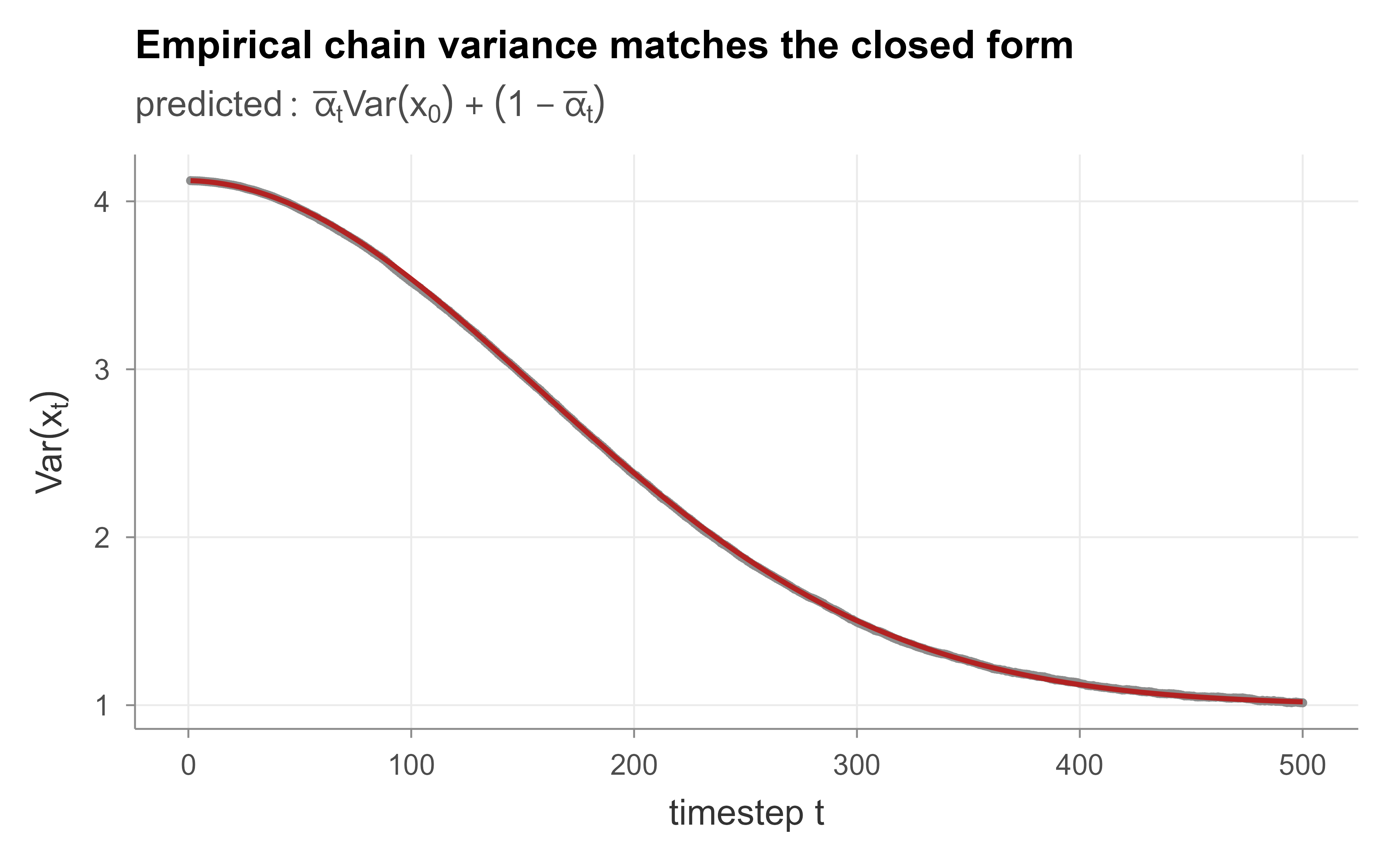
Figure 43.2: Closed form verification. Points are the empirical variance of the simulated forward chain at each timestep; the line is the predicted marginal variance 1 minus alpha-bar_t. They coincide, confirming the variance preserving property.

Figure 43.2 plots the empirical variance of the step by step simulation against the closed form prediction $\bar{\alpha}_t\,\mathrm{Var}(\mathbf{x}_0) + (1-\bar{\alpha}_t)$ from Equation 43.4. The two lie on top of each other, and the printed maximum absolute error is tiny, confirming that the iterated Gaussian steps really do compose into the single jump Equation 43.5. The terminal variance lands at approximately one, the hallmark of the variance preserving schedule. This is the foundation on which the entire training and sampling machinery rests.

The neural noise predictor itself would slot in here as the only learned component. For completeness, the training loop in a deep learning framework looks like the following (shown but not run, since it needs a backend such as torch, Chapter 46 discusses the same stack).

Show code

## Sketch of the simplified DDPM training step (pseudocode-level torch).
## eps_model is a network mapping (x_t, t) -> predicted noise.
train_step <- function(x0, eps_model, abar, optimizer) {
  n  <- nrow(x0)
  t  <- sample.int(length(abar), n, replace = TRUE)      # random timesteps
  eps <- torch_randn_like(x0)                            # true noise
  a   <- torch_sqrt(abar[t])$view(c(n, 1))
  b   <- torch_sqrt(1 - abar[t])$view(c(n, 1))
  xt  <- a * x0 + b * eps                                # eq-diffusion-reparam
  pred <- eps_model(xt, t)                               # predict the noise
  loss <- nnf_mse_loss(pred, eps)                        # eq-diffusion-simple
  optimizer$zero_grad(); loss$backward(); optimizer$step()
  loss$item()
}

The mapping from the math to the code is one to one: xt is Equation 43.5, the loss is Equation 43.15, and at generation time one would iterate Equation 43.16 or Equation 43.17. Everything else in this chapter is the justification for why those few lines suffice.

43.8 Summary

Diffusion models generate data by learning to reverse a fixed Gaussian noising process. The forward chain Equation 43.1 has a closed form marginal Equation 43.4 that lets us add any amount of noise in one step and makes the variational bound Equation 43.10 a sum of tractable Gaussian KL divergences. Reparameterizing the reverse mean in terms of the added noise collapses that bound into the plain regression objective Equation 43.15: predict the noise with mean squared error. Sampling runs the learned reverse chain, either stochastically (DDPM, Equation 43.16) or deterministically and quickly (DDIM, Equation 43.17). The model is a fixed encoder hierarchical VAE, a denoising score matcher (Chapter 32), and the discretization of a reverse time SDE all at once, which is why it is both easy to train and rich to analyze. The base R demonstration confirmed the single fact everything depends on, that the iterated forward steps compose into the closed form variance schedule, without needing any deep learning machinery.

# Diffusion Models {#sec-diffusion} ```{r} #| include: false source("_common.R") ``` Picture a clear photograph. Now imagine sprinkling a little static onto it, then a little more, and a little more, until after a few hundred steps nothing is left but pure television snow. That destruction is easy: anyone can add noise. The hard and interesting question is whether a model can learn to run the tape backward, starting from snow and removing noise one careful step at a time until a brand new, never seen photograph emerges. A diffusion model is exactly a learned procedure for reversing noise. It is trained on the easy forward direction, where we know precisely how much noise we added, and it uses that knowledge to take small, confident steps in the hard reverse direction. This idea now powers most state of the art image, audio, and video generators. It belongs to the family of generative models (@sec-generative-models) alongside variational autoencoders and generative adversarial networks, but it reaches the goal, a model you can sample from, by a route that is unusually stable to train and unusually clean to analyze. The reason is that every quantity we need has a closed form. We never have to fight an adversary the way a GAN does, and we never have to approximate an intractable posterior the way a plain VAE does. We simply teach a network to predict the noise that was added, and almost everything else follows from Gaussian algebra. ::: {.callout-tip title="Intuition"} Adding noise is a one way street that is trivial to walk forward. A diffusion model learns a guidebook for walking back up that street. Because each forward step is a tiny Gaussian nudge, each backward step is also approximately Gaussian, and predicting one small nudge at a time is far easier than inventing a whole image in one shot. ::: This chapter develops the model in the order that makes the math honest. We first define the forward noising process and derive its closed form marginal, which is the single fact that makes everything else tractable. We then write the reverse process as a learned Markov chain, connect its training objective to the evidence lower bound (ELBO), and show how that objective collapses into a strikingly simple noise prediction loss. From there we cover sampling (the ancestral DDPM sampler and the deterministic DDIM shortcut), the relationships to VAEs (@sec-autoencoders) and to score based stochastic differential equations, and classifier free guidance. A runnable base R demonstration closes the chapter by forward diffusing a one dimensional distribution and verifying the closed form variance schedule numerically. ## The forward process Let $\mathbf{x}_0 \in \mathbb{R}^d$ be a data point drawn from the unknown data distribution $q(\mathbf{x}_0)$. The forward process is a fixed (not learned) Markov chain that gradually adds Gaussian noise over $T$ steps, producing latents $\mathbf{x}_1, \dots, \mathbf{x}_T$. Each step is $$ q(\mathbf{x}_t \mid \mathbf{x}_{t-1}) = \mathcal{N}\!\big(\mathbf{x}_t;\ \sqrt{1-\beta_t}\,\mathbf{x}_{t-1},\ \beta_t \mathbf{I}\big), $$ {#eq-diffusion-forward-step} where the variances $\beta_1, \dots, \beta_T \in (0,1)$ form a fixed schedule that usually increases with $t$. The factor $\sqrt{1-\beta_t}$ in the mean shrinks the previous state slightly while $\beta_t \mathbf{I}$ injects fresh noise; this particular pairing is what keeps the total variance from exploding, as we verify below. The full forward chain factorizes as $$ q(\mathbf{x}_{1:T} \mid \mathbf{x}_0) = \prod_{t=1}^{T} q(\mathbf{x}_t \mid \mathbf{x}_{t-1}). $$ {#eq-diffusion-forward-chain} If $T$ is large and the schedule is chosen so that $\prod_t (1-\beta_t)$ becomes tiny, then $q(\mathbf{x}_T)$ is essentially a standard normal $\mathcal{N}(\mathbf{0}, \mathbf{I})$ regardless of where $\mathbf{x}_0$ started. That terminal distribution is what we will sample from at generation time, so it must be something we can sample trivially, and the standard normal is. ::: {.callout-important title="Key idea"} The forward process has no parameters to learn. It is a known corruption recipe. All of the learning happens in the reverse process, whose only job is to undo this recipe one step at a time. ::: ### The closed form marginal The chain in @eq-diffusion-forward-chain looks like it requires $t$ sequential samples to reach $\mathbf{x}_t$. It does not. Because the composition of Gaussians is Gaussian, we can jump from $\mathbf{x}_0$ to any $\mathbf{x}_t$ in a single step. Define $$ \alpha_t = 1 - \beta_t, \qquad \bar{\alpha}_t = \prod_{s=1}^{t} \alpha_s . $$ {#eq-diffusion-alphabar} The claim is the marginal $$ q(\mathbf{x}_t \mid \mathbf{x}_0) = \mathcal{N}\!\big(\mathbf{x}_t;\ \sqrt{\bar{\alpha}_t}\,\mathbf{x}_0,\ (1-\bar{\alpha}_t)\mathbf{I}\big). $$ {#eq-diffusion-marginal} This is the workhorse of the whole theory. Let us derive it. Using the reparameterization trick, @eq-diffusion-forward-step says $$ \mathbf{x}_t = \sqrt{\alpha_t}\,\mathbf{x}_{t-1} + \sqrt{1-\alpha_t}\,\boldsymbol{\epsilon}_{t-1}, \qquad \boldsymbol{\epsilon}_{t-1} \sim \mathcal{N}(\mathbf{0}, \mathbf{I}), $$ and the noise variables at different steps are independent. Substitute one step into the next: $$ \begin{aligned} \mathbf{x}_t &= \sqrt{\alpha_t}\big(\sqrt{\alpha_{t-1}}\,\mathbf{x}_{t-2} + \sqrt{1-\alpha_{t-1}}\,\boldsymbol{\epsilon}_{t-2}\big) + \sqrt{1-\alpha_t}\,\boldsymbol{\epsilon}_{t-1} \\ &= \sqrt{\alpha_t \alpha_{t-1}}\,\mathbf{x}_{t-2} + \underbrace{\sqrt{\alpha_t(1-\alpha_{t-1})}\,\boldsymbol{\epsilon}_{t-2} + \sqrt{1-\alpha_t}\,\boldsymbol{\epsilon}_{t-1}}_{\text{sum of two independent Gaussians}}. \end{aligned} $$ The bracketed term is a sum of two independent zero mean Gaussians, so it is itself zero mean Gaussian with variance equal to the sum of the variances, $$ \alpha_t(1-\alpha_{t-1}) + (1-\alpha_t) = 1 - \alpha_t \alpha_{t-1}. $$ Therefore $\mathbf{x}_t = \sqrt{\alpha_t \alpha_{t-1}}\,\mathbf{x}_{t-2} + \sqrt{1-\alpha_t\alpha_{t-1}}\,\bar{\boldsymbol{\epsilon}}$ with $\bar{\boldsymbol{\epsilon}} \sim \mathcal{N}(\mathbf{0},\mathbf{I})$. Iterating this collapse all the way down to $\mathbf{x}_0$ replaces the product $\alpha_t \alpha_{t-1} \cdots$ with $\bar{\alpha}_t$, giving $$ \mathbf{x}_t = \sqrt{\bar{\alpha}_t}\,\mathbf{x}_0 + \sqrt{1-\bar{\alpha}_t}\,\boldsymbol{\epsilon}, \qquad \boldsymbol{\epsilon} \sim \mathcal{N}(\mathbf{0}, \mathbf{I}), $$ {#eq-diffusion-reparam} which is precisely @eq-diffusion-marginal in sampled form. Two consequences are immediate. First, the signal coefficient $\sqrt{\bar{\alpha}_t}$ and the noise coefficient $\sqrt{1-\bar{\alpha}_t}$ always satisfy $\bar{\alpha}_t + (1-\bar{\alpha}_t) = 1$, so the marginal variance of any coordinate stays bounded as $t$ grows (this is the variance preserving property we verify numerically later). Second, training never needs the intermediate latents: to get a training pair at any timestep $t$ we draw one $\boldsymbol{\epsilon}$ and apply @eq-diffusion-reparam directly. ::: {.callout-note} The clean separation in @eq-diffusion-reparam, a deterministic scaling of the data plus a single Gaussian noise vector, is the reason diffusion training is cheap. We can sample any noise level $t$ in $O(1)$ work rather than simulating $t$ chained steps. ::: ### The forward posterior is Gaussian To build a reverse model we need to know, conditioned on the original $\mathbf{x}_0$, what the previous state $\mathbf{x}_{t-1}$ looked like given $\mathbf{x}_t$. This forward posterior $q(\mathbf{x}_{t-1} \mid \mathbf{x}_t, \mathbf{x}_0)$ is tractable and Gaussian. By Bayes rule within the chain, $$ q(\mathbf{x}_{t-1} \mid \mathbf{x}_t, \mathbf{x}_0) = \mathcal{N}\!\big(\mathbf{x}_{t-1};\ \tilde{\boldsymbol{\mu}}_t(\mathbf{x}_t, \mathbf{x}_0),\ \tilde{\beta}_t \mathbf{I}\big), $$ {#eq-diffusion-posterior} with $$ \tilde{\boldsymbol{\mu}}_t = \frac{\sqrt{\bar{\alpha}_{t-1}}\,\beta_t}{1-\bar{\alpha}_t}\,\mathbf{x}_0 + \frac{\sqrt{\alpha_t}\,(1-\bar{\alpha}_{t-1})}{1-\bar{\alpha}_t}\,\mathbf{x}_t, \qquad \tilde{\beta}_t = \frac{1-\bar{\alpha}_{t-1}}{1-\bar{\alpha}_t}\,\beta_t . $$ {#eq-diffusion-posterior-params} These follow from multiplying the two Gaussians $q(\mathbf{x}_t\mid\mathbf{x}_{t-1})$ and $q(\mathbf{x}_{t-1}\mid\mathbf{x}_0)$ and completing the square in $\mathbf{x}_{t-1}$; the algebra is the standard Gaussian product identity, and the resulting mean is a precision weighted average of the two contributing means. The point of @eq-diffusion-posterior is that the true reverse step, when we are allowed to peek at $\mathbf{x}_0$, is exactly Gaussian. The job of the network will be to match this Gaussian without peeking. ## The reverse process and the ELBO At generation time we do not know $\mathbf{x}_0$, so we approximate the reverse step with a learned Gaussian whose mean is a neural network $\boldsymbol{\mu}_\theta$ and whose covariance is fixed (or also learned), $$ p_\theta(\mathbf{x}_{t-1} \mid \mathbf{x}_t) = \mathcal{N}\!\big(\mathbf{x}_{t-1};\ \boldsymbol{\mu}_\theta(\mathbf{x}_t, t),\ \sigma_t^2 \mathbf{I}\big), $$ {#eq-diffusion-reverse-step} starting from $p(\mathbf{x}_T) = \mathcal{N}(\mathbf{0}, \mathbf{I})$ and running $t = T, T-1, \dots, 1$. The generative model is the marginal $p_\theta(\mathbf{x}_0) = \int p(\mathbf{x}_T)\prod_t p_\theta(\mathbf{x}_{t-1}\mid\mathbf{x}_t)\, d\mathbf{x}_{1:T}$. This is structurally a hierarchical VAE with $T$ stochastic layers, a fixed encoder (the forward process), and a learned decoder (the reverse process). As in any latent variable model, the marginal likelihood is intractable, so we maximize a variational lower bound. The same Jensen inequality used for the VAE in @sec-autoencoders gives the ELBO $$ \log p_\theta(\mathbf{x}_0) \ \ge\ \mathbb{E}_q\!\left[\log \frac{p_\theta(\mathbf{x}_{0:T})}{q(\mathbf{x}_{1:T}\mid\mathbf{x}_0)}\right] =: -\mathcal{L}. $$ {#eq-diffusion-elbo} The negative ELBO $\mathcal{L}$ is what we minimize. Because both numerator and denominator factorize over $t$, $\mathcal{L}$ decomposes into per step terms. After regrouping (the standard Sohl-Dickstein/Ho derivation), the bound becomes a sum of KL divergences between Gaussians: $$ \mathcal{L} = \underbrace{D_{\mathrm{KL}}\!\big(q(\mathbf{x}_T\mid\mathbf{x}_0)\,\|\,p(\mathbf{x}_T)\big)}_{L_T} + \sum_{t=2}^{T}\underbrace{\mathbb{E}_q\, D_{\mathrm{KL}}\!\big(q(\mathbf{x}_{t-1}\mid\mathbf{x}_t,\mathbf{x}_0)\,\|\,p_\theta(\mathbf{x}_{t-1}\mid\mathbf{x}_t)\big)}_{L_{t-1}} - \underbrace{\mathbb{E}_q \log p_\theta(\mathbf{x}_0\mid\mathbf{x}_1)}_{L_0}. $$ {#eq-diffusion-elbo-decomp} The first term $L_T$ has no parameters: it measures how close the fully noised data is to the standard normal prior, and with a well chosen schedule it is negligible. The reconstruction term $L_0$ handles the final decode to data space. The interesting work is in the middle terms $L_{t-1}$, each of which is a KL between two Gaussians: the tractable forward posterior @eq-diffusion-posterior and the learned reverse step @eq-diffusion-reverse-step. ### From KL divergence to noise prediction For two Gaussians with the same covariance $\sigma_t^2 \mathbf{I}$, the KL divergence reduces to a scaled squared distance between their means, $$ L_{t-1} = \mathbb{E}_q\!\left[\frac{1}{2\sigma_t^2}\,\big\|\tilde{\boldsymbol{\mu}}_t(\mathbf{x}_t,\mathbf{x}_0) - \boldsymbol{\mu}_\theta(\mathbf{x}_t, t)\big\|^2\right] + \text{const}. $$ {#eq-diffusion-Lt-mean} So the network's mean $\boldsymbol{\mu}_\theta$ should match the posterior mean $\tilde{\boldsymbol{\mu}}_t$. Here is the elegant simplification. Solve @eq-diffusion-reparam for $\mathbf{x}_0 = (\mathbf{x}_t - \sqrt{1-\bar{\alpha}_t}\,\boldsymbol{\epsilon})/\sqrt{\bar{\alpha}_t}$ and substitute into $\tilde{\boldsymbol{\mu}}_t$ from @eq-diffusion-posterior-params. After simplification the posterior mean depends on $\mathbf{x}_t$ and the noise $\boldsymbol{\epsilon}$ only: $$ \tilde{\boldsymbol{\mu}}_t = \frac{1}{\sqrt{\alpha_t}}\left(\mathbf{x}_t - \frac{\beta_t}{\sqrt{1-\bar{\alpha}_t}}\,\boldsymbol{\epsilon}\right). $$ {#eq-diffusion-mu-eps} This suggests parameterizing the network not as a mean predictor but as a noise predictor $\boldsymbol{\epsilon}_\theta(\mathbf{x}_t, t)$ that guesses which $\boldsymbol{\epsilon}$ was added, and then setting $$ \boldsymbol{\mu}_\theta(\mathbf{x}_t, t) = \frac{1}{\sqrt{\alpha_t}}\left(\mathbf{x}_t - \frac{\beta_t}{\sqrt{1-\bar{\alpha}_t}}\,\boldsymbol{\epsilon}_\theta(\mathbf{x}_t, t)\right). $$ {#eq-diffusion-mu-theta} Plugging @eq-diffusion-mu-eps and @eq-diffusion-mu-theta into @eq-diffusion-Lt-mean, the difference of means becomes a difference of noise vectors, and $L_{t-1}$ turns into $$ L_{t-1} = \mathbb{E}_{\mathbf{x}_0, \boldsymbol{\epsilon}}\!\left[\frac{\beta_t^2}{2\sigma_t^2\,\alpha_t\,(1-\bar{\alpha}_t)}\,\big\|\boldsymbol{\epsilon} - \boldsymbol{\epsilon}_\theta(\sqrt{\bar{\alpha}_t}\mathbf{x}_0 + \sqrt{1-\bar{\alpha}_t}\boldsymbol{\epsilon},\ t)\big\|^2\right]. $$ {#eq-diffusion-Lt-weighted} Every term is now a weighted mean squared error between the true noise and the predicted noise. Ho, Jain, and Abbeel (2020) observed that simply dropping the awkward per step weight and using the unweighted version trains better in practice, giving the famous simplified objective $$ \mathcal{L}_{\text{simple}} = \mathbb{E}_{t,\,\mathbf{x}_0,\,\boldsymbol{\epsilon}}\!\left[\big\|\boldsymbol{\epsilon} - \boldsymbol{\epsilon}_\theta(\sqrt{\bar{\alpha}_t}\,\mathbf{x}_0 + \sqrt{1-\bar{\alpha}_t}\,\boldsymbol{\epsilon},\ t)\big\|^2\right], $$ {#eq-diffusion-simple} with $t$ drawn uniformly over $\{1, \dots, T\}$. This is just regression. The network sees a noisy input and a timestep and predicts the noise; the loss is plain squared error. There is no adversary and no sampling inside the loss, which is why diffusion training is so stable. ::: {.callout-important title="Key idea"} The entire training procedure is: pick a random data point, pick a random timestep, add a known amount of Gaussian noise, and train a network to predict that noise with mean squared error. The ELBO derivation justifies this, but the implementation is a few lines. ::: ### Connection to denoising score matching The noise prediction objective is the same thing as score matching (@sec-density-estimation), viewed through a change of variable. The score of the noised marginal is the gradient of its log density, $\mathbf{s}(\mathbf{x}_t) = \nabla_{\mathbf{x}_t} \log q(\mathbf{x}_t)$. For the Gaussian marginal @eq-diffusion-marginal, that score equals $-\boldsymbol{\epsilon}/\sqrt{1-\bar{\alpha}_t}$ in expectation, so a network that predicts $\boldsymbol{\epsilon}$ is, up to the scaling $-1/\sqrt{1-\bar{\alpha}_t}$, predicting the score. Minimizing @eq-diffusion-simple is therefore denoising score matching across a continuum of noise levels. This is the bridge to the score based view we describe next, and it is why people use the words "score model" and "diffusion model" almost interchangeably. ## Sampling Once $\boldsymbol{\epsilon}_\theta$ is trained, generation runs the learned reverse chain. The ancestral (DDPM) sampler starts from $\mathbf{x}_T \sim \mathcal{N}(\mathbf{0}, \mathbf{I})$ and, for $t = T, \dots, 1$, draws $$ \mathbf{x}_{t-1} = \frac{1}{\sqrt{\alpha_t}}\left(\mathbf{x}_t - \frac{\beta_t}{\sqrt{1-\bar{\alpha}_t}}\,\boldsymbol{\epsilon}_\theta(\mathbf{x}_t, t)\right) + \sigma_t\,\mathbf{z}, \qquad \mathbf{z} \sim \mathcal{N}(\mathbf{0}, \mathbf{I}), $$ {#eq-diffusion-ddpm-sampler} with $\mathbf{z} = \mathbf{0}$ at the last step, and $\sigma_t^2$ typically set to $\beta_t$ or to the posterior variance $\tilde{\beta}_t$. The deterministic mean here is exactly @eq-diffusion-mu-theta, and the added $\sigma_t \mathbf{z}$ is the stochastic part of the reverse step. The drawback is cost: faithful samples often need hundreds or thousands of steps, each a full network evaluation. DDIM (Song, Meng, Ermon 2021) removes most of that cost. It defines a non Markovian forward process that shares the same marginals @eq-diffusion-marginal, so the same trained $\boldsymbol{\epsilon}_\theta$ applies, but whose reverse step can be made deterministic. The DDIM update first estimates the clean signal $\hat{\mathbf{x}}_0 = (\mathbf{x}_t - \sqrt{1-\bar{\alpha}_t}\,\boldsymbol{\epsilon}_\theta)/\sqrt{\bar{\alpha}_t}$, then re-noises it to level $t-1$: $$ \mathbf{x}_{t-1} = \sqrt{\bar{\alpha}_{t-1}}\,\hat{\mathbf{x}}_0 + \sqrt{1-\bar{\alpha}_{t-1}}\,\boldsymbol{\epsilon}_\theta(\mathbf{x}_t, t). $$ {#eq-diffusion-ddim} Because there is no injected noise, the map from $\mathbf{x}_T$ to $\mathbf{x}_0$ is deterministic, the same seed always gives the same image, and one can skip timesteps aggressively, generating in 10 to 50 steps instead of 1000. DDIM trades a little sample diversity for a large speedup and is the practical default for many systems. ::: {.callout-tip title="Practical note"} The DDPM sampler is stochastic and tends to give more diverse, slightly higher fidelity samples at high step counts; the DDIM sampler is deterministic and far faster at low step counts. Switching between them needs no retraining, since both use the same $\boldsymbol{\epsilon}_\theta$. ::: ## Connections: VAEs and score based SDEs Two viewpoints unify diffusion with the rest of the book. As a hierarchical VAE (@sec-autoencoders), a diffusion model is a VAE whose encoder is fixed and hand designed (the noising chain) rather than learned, with $T$ latent layers instead of one. This is why the same ELBO machinery applies verbatim. The crucial difference from an ordinary VAE is that the fixed encoder has a closed form posterior @eq-diffusion-posterior, so the KL terms are exact Gaussian KLs with no amortization gap and no posterior collapse. As a stochastic differential equation, take the limit $T \to \infty$ with infinitesimal steps. The discrete forward chain becomes a continuous time SDE $$ d\mathbf{x} = -\tfrac{1}{2}\beta(t)\,\mathbf{x}\,dt + \sqrt{\beta(t)}\,d\mathbf{w}, $$ where $\mathbf{w}$ is a Wiener process. Anderson's reverse time SDE theorem says the corresponding reverse process is $$ d\mathbf{x} = \big[-\tfrac{1}{2}\beta(t)\mathbf{x} - \beta(t)\,\nabla_{\mathbf{x}}\log q_t(\mathbf{x})\big]dt + \sqrt{\beta(t)}\,d\bar{\mathbf{w}}, $$ which needs only the score $\nabla_{\mathbf{x}}\log q_t$, exactly what $\boldsymbol{\epsilon}_\theta$ learns. There is also a deterministic probability flow ODE with the same marginals, which is the continuous time cousin of DDIM and connects diffusion to normalizing flows and to Gaussian process style continuous dynamics (@sec-gaussian-process-reg). This SDE picture is what licenses the many fast ODE solvers (for example DPM-Solver) used in production. ## Classifier free guidance To steer generation with a condition $c$ (a class label or a text prompt), one trains a single conditional network $\boldsymbol{\epsilon}_\theta(\mathbf{x}_t, t, c)$ but randomly drops the condition during training (replacing $c$ with a null token) so the same weights also learn the unconditional score $\boldsymbol{\epsilon}_\theta(\mathbf{x}_t, t, \varnothing)$. At sampling time the two predictions are combined with a guidance weight $w \ge 0$, $$ \tilde{\boldsymbol{\epsilon}} = (1+w)\,\boldsymbol{\epsilon}_\theta(\mathbf{x}_t, t, c) - w\,\boldsymbol{\epsilon}_\theta(\mathbf{x}_t, t, \varnothing), $$ which extrapolates away from the unconditional direction and toward the conditional one, sharpening adherence to $c$ at some cost in diversity. This classifier free scheme (Ho and Salimans 2022) avoids training a separate classifier on noisy inputs and is the standard conditioning method in modern text to image systems. ## Practical considerations A few facts matter when building or reading about these models. - **Architecture.** $\boldsymbol{\epsilon}_\theta$ for images is almost always a U-Net with residual blocks and self attention (@sec-transformers); the timestep $t$ enters through a sinusoidal embedding added to each block. The network shares weights across all timesteps. These pieces need a GPU and a deep learning backend, so the neural code in this chapter is shown unevaluated. - **Noise schedule.** A linear $\beta_t$ schedule works but a cosine schedule for $\bar{\alpha}_t$ usually trains better by spending more steps at low noise. The schedule fully determines $\bar{\alpha}_t$ and hence the forward marginals. - **Cost.** Training is cheap per step (one forward and backward pass on a noisy image) but sampling is expensive (one network call per reverse step). DDIM and ODE solvers cut sampling steps by one to two orders of magnitude. - **Failure modes.** Too few sampling steps gives blurry or artifact ridden outputs; a poorly tuned schedule wastes capacity at noise levels that carry little signal; overly large guidance weights produce oversaturated, low diversity samples. Unlike GANs, diffusion models rarely suffer mode collapse, which is one of their main attractions. - **Likelihoods.** The ELBO gives a real (if loose) bound on log likelihood, so diffusion models can report calibrated likelihoods, something GANs cannot. ::: {.callout-warning} The simplified loss @eq-diffusion-simple drops the ELBO weights, so the quantity you minimize is no longer a valid likelihood bound. It generates better samples but you should not read $\mathcal{L}_{\text{simple}}$ as a log likelihood. To report likelihoods, use the weighted variational bound @eq-diffusion-elbo-decomp. ::: ## A runnable demonstration: forward diffusion in one dimension The neural reverse model needs a GPU, but the forward process and its closed form marginal are pure algebra that we can verify exactly in base R. The demonstration below takes a simple non Gaussian one dimensional distribution (a two component mixture), runs the forward chain @eq-diffusion-forward-step step by step on a large sample, and checks two things: that the empirical mean and variance at each timestep match the closed form $\sqrt{\bar{\alpha}_t}\,\mathbf{x}_0$ scaling and the $1-\bar{\alpha}_t$ variance growth predicted by @eq-diffusion-marginal, and that the distribution morphs from a clearly bimodal shape into a standard normal. ```{r} #| label: fig-diffusion-forward #| fig-cap: "Forward diffusion of a one dimensional two component mixture. The histograms show the sample at four noise levels: the bimodal data gradually relax into a single standard normal bump as t increases." #| fig-width: 7 #| fig-height: 4.5 set.seed(1301) ## ---- A simple non-Gaussian data distribution: a two-component mixture ---- n <- 40000 comp <- rbinom(n, 1, 0.5) x0 <- ifelse(comp == 1, rnorm(n, mean = -2.0, sd = 0.35), rnorm(n, mean = 2.0, sd = 0.35)) ## ---- Forward noise schedule (linear betas, the original DDPM choice) ---- TT <- 500 beta <- seq(1e-4, 0.02, length.out = TT) # increasing variances alpha <- 1 - beta abar <- cumprod(alpha) # alpha-bar_t (eq-diffusion-alphabar) ## ---- Run the forward Markov chain step by step (no closed form used) ---- ## x_t = sqrt(alpha_t) x_{t-1} + sqrt(beta_t) * noise X <- x0 snapshots <- list() keep <- c(1, 100, 250, 500) # timesteps to visualize for (t in seq_len(TT)) { X <- sqrt(alpha[t]) * X + sqrt(beta[t]) * rnorm(n) if (t %in% keep) snapshots[[as.character(t)]] <- X } ## ---- Assemble a tidy data frame for plotting ---- df <- do.call(rbind, lapply(keep, function(t) data.frame(value = snapshots[[as.character(t)]], step = factor(paste0("t = ", t), levels = paste0("t = ", keep))))) ggplot(df, aes(value)) + geom_histogram(aes(y = after_stat(density)), bins = 60, fill = "grey75", colour = "white", linewidth = 0.2) + facet_wrap(~ step, nrow = 1) + stat_function(fun = dnorm, colour = "firebrick", linewidth = 0.7) + labs(x = expression(x[t]), y = "density", title = "Forward diffusion turns a bimodal distribution into N(0, 1)", subtitle = "Red curve is the standard normal target") + theme_book() ``` @fig-diffusion-forward shows the sample collapsing onto the standard normal (the red curve) as the chain progresses. The key quantitative check is that the simulated chain, which never used the closed form, agrees with the closed form marginal @eq-diffusion-marginal. We verify the variance schedule directly. ```{r} #| label: fig-diffusion-variance #| fig-cap: "Closed form verification. Points are the empirical variance of the simulated forward chain at each timestep; the line is the predicted marginal variance 1 minus alpha-bar_t. They coincide, confirming the variance preserving property." #| fig-width: 6.5 #| fig-height: 4 ## ---- Re-run the chain and record the empirical variance at every step ---- ## Closed form (eq-diffusion-marginal): Var(x_t) = abar_t * Var(x_0) + (1 - abar_t). ## Because we standardize x0 to unit variance below, the prediction is simply ## Var(x_t) = abar_t * var(x0) + (1 - abar_t). var_x0 <- var(x0) X <- x0 emp_var <- numeric(TT) for (t in seq_len(TT)) { X <- sqrt(alpha[t]) * X + sqrt(beta[t]) * rnorm(n) emp_var[t] <- var(X) } pred_var <- abar * var_x0 + (1 - abar) vdf <- data.frame(t = seq_len(TT), empirical = emp_var, predicted = pred_var) ## ---- Numerical agreement ---- max_abs_err <- max(abs(vdf$empirical - vdf$predicted)) cat(sprintf("Maximum |empirical - predicted| variance error: %.4f\n", max_abs_err)) cat(sprintf("Var(x_0) = %.3f, Var(x_T) = %.3f (target ~ 1.0)\n", var_x0, emp_var[TT])) ggplot(vdf, aes(t)) + geom_point(aes(y = empirical), colour = "grey55", size = 0.7) + geom_line(aes(y = predicted), colour = "firebrick", linewidth = 0.8) + labs(x = "timestep t", y = expression(Var(x[t])), title = "Empirical chain variance matches the closed form", subtitle = expression(predicted: ~ bar(alpha)[t] * Var(x[0]) + (1 - bar(alpha)[t]))) + theme_book() ``` @fig-diffusion-variance plots the empirical variance of the step by step simulation against the closed form prediction $\bar{\alpha}_t\,\mathrm{Var}(\mathbf{x}_0) + (1-\bar{\alpha}_t)$ from @eq-diffusion-marginal. The two lie on top of each other, and the printed maximum absolute error is tiny, confirming that the iterated Gaussian steps really do compose into the single jump @eq-diffusion-reparam. The terminal variance lands at approximately one, the hallmark of the variance preserving schedule. This is the foundation on which the entire training and sampling machinery rests. The neural noise predictor itself would slot in here as the only learned component. For completeness, the training loop in a deep learning framework looks like the following (shown but not run, since it needs a backend such as torch, @sec-bayesian-deep-learning discusses the same stack). ```{r} #| eval: false ## Sketch of the simplified DDPM training step (pseudocode-level torch). ## eps_model is a network mapping (x_t, t) -> predicted noise. train_step <- function(x0, eps_model, abar, optimizer) { n <- nrow(x0) t <- sample.int(length(abar), n, replace = TRUE) # random timesteps eps <- torch_randn_like(x0) # true noise a <- torch_sqrt(abar[t])$view(c(n, 1)) b <- torch_sqrt(1 - abar[t])$view(c(n, 1)) xt <- a * x0 + b * eps # eq-diffusion-reparam pred <- eps_model(xt, t) # predict the noise loss <- nnf_mse_loss(pred, eps) # eq-diffusion-simple optimizer$zero_grad(); loss$backward(); optimizer$step() loss$item() } ``` The mapping from the math to the code is one to one: `xt` is @eq-diffusion-reparam, the loss is @eq-diffusion-simple, and at generation time one would iterate @eq-diffusion-ddpm-sampler or @eq-diffusion-ddim. Everything else in this chapter is the justification for why those few lines suffice. ## Summary Diffusion models generate data by learning to reverse a fixed Gaussian noising process. The forward chain @eq-diffusion-forward-step has a closed form marginal @eq-diffusion-marginal that lets us add any amount of noise in one step and makes the variational bound @eq-diffusion-elbo-decomp a sum of tractable Gaussian KL divergences. Reparameterizing the reverse mean in terms of the added noise collapses that bound into the plain regression objective @eq-diffusion-simple: predict the noise with mean squared error. Sampling runs the learned reverse chain, either stochastically (DDPM, @eq-diffusion-ddpm-sampler) or deterministically and quickly (DDIM, @eq-diffusion-ddim). The model is a fixed encoder hierarchical VAE, a denoising score matcher (@sec-density-estimation), and the discretization of a reverse time SDE all at once, which is why it is both easy to train and rich to analyze. The base R demonstration confirmed the single fact everything depends on, that the iterated forward steps compose into the closed form variance schedule, without needing any deep learning machinery.